Abstract
Due to the variable nature of wind resources, the increasing penetration level of wind power will have a significant impact on the operation and planning of the electric power system. Energy storage systems are considered an effective way to compensate for the variability of wind generation. This paper presents a detailed production cost simulation model to evaluate the economic value of compressed air energy storage (CAES) in systems with large-scale wind power generation. The co-optimization of energy and ancillary services markets is implemented in order to analyze the impacts of CAES, not only on energy supply, but also on system operating reserves. Both hourly and 5-minute simulations are considered to capture the economic performance of CAES in the day-ahead (DA) and real-time (RT) markets. The generalized network flow formulation is used to model the characteristics of CAES in detail. The proposed model is applied on a modified IEEE 24-bus reliability test system. The numerical example shows that besides the economic benefits gained through energy arbitrage in the DA market, CAES can also generate significant profits by providing reserves, compensating for wind forecast errors and intra-hour fluctuation, and participating in the RT market.
1. Introduction
In the last decade, there has been significant growth in wind capacity in the US because of advancements in wind generation technology, government subsidies, and other policy incentives [1]. With the focus on promoting the use of renewable energy, the efficient and cost-effective integration of wind energy to the grid is becoming increasingly important.
A number of studies have been carried out to evaluate the possibility of using various kinds of Energy Storage Systems (ESS) to offset the wind generation variability [2,3,4,5,6]. Energy storage systems convert electric energy into various kinds of storable intermediary energies, such as mechanical, potential, chemical, biological, electrical, and thermal, and then convert them back to electric energy. The most common energy storage technologies include pump storage, flywheels, battery, compressed air storage, thermal storage, and hydrogen storage. A comparison of energy storage systems is provided in [7].
Energy storage systems can be used to perform energy arbitrage, i.e., storing energy at off-peak hours and selling it at peak hours to increase profits. Energy storage can also be used to provide high-value ancillary services, enhance the stability of the electric system, and serve as a substitute for transmission line investment. Moreover, with significant penetration of wind generation, thermal units need to constantly vary their generation outputs to maintain frequency performance. The excessive cycling of these coal- and natural gas- fired units will cause faster aging, higher forced outage rates, and extra maintenance costs. As most energy storage systems can provide fast-ramping reserves, they are ideal options to counterbalance the effects of wind generation. At high wind penetration levels and/or imperfect wind forecasts, the value and use of energy storage increase [8].
One major obstacle of the wide adoption of energy storage systems is their economic justification. Converting electric energy into another form and converting it back incurs high energy losses and costs. Pumped hydro and compressed air energy storage (CAES) are among the most economically competitive high capacity energy storage options. Pumped hydro storage is the most widespread energy storage system today, with about 127 GW of installed capacity which accounts for around 3% of global generation capacity [9]. However, pumped hydro is very site-specific and has adverse effects on the environment [10], which limit its application. CAES is a modification of the gas turbine (GT) technology. Off-peak (low-cost) electrical power is used to compress air into an underground air storage cavern. The compressed air is then preheated by a natural gas fired burner to power the gas turbine when the energy price is high. Compared with many other energy storage techniques, the ability of CAES to support large-scale power application with relatively low capital and maintenance costs per unit energy makes it attractive [7]. What is more, compared to pumped hydro, CAES is less site-specific because a large part of the U.S. has geologic conditions favorable for underground air storage [6,11]. In this article, a production cost simulation model is proposed to evaluate the economic value of CAES in systems with high wind penetration levels.
There are two operating scenarios for CAES: co-located with wind farms, or located near the load center [3]. Wind-rich areas are generally remote from the load center, so the wind energy needs to be transferred via long-distance transmission lines. The existing transmission system linking wind farms and load centers are often congested as they were not designed for the transfer capability required by the wind growth. When storage is located at the load center, it can be used as an alternative to transmission expansion by conducting energy arbitrage, which utilizes the transmission system to transfer low cost wind power during off-peak hours. When storage is located near the remote wind sites, it can also take advantage of the time-varying spot prices caused by high-penetration of wind power and ensure the efficient use of wind generation. One of the objectives of this paper is to identify the impact of the two operating scenarios on the economic value of CAES.
Several operational impacts should be considered when evaluating the viability of incorporating energy storage systems to address wind integration issues: load following, scheduling, reserve requirement, ramping requirement, and wind forecast errors and intra-hour fluctuation [5]. While significant efforts have been made to evaluate the benefits of ESS on load following and scheduling via hourly energy market simulations [2,3,4,5,9], the contributions of ESS on reserves and ramping requirements have not been given enough consideration. In some studies, historical energy and reserves prices are used as input to evaluate CAES’s value of providing reserves and energy [12,13]. However, this approach cannot simulate the impacts of CAES generation and siting on the system dispatch and congestions patterns, which in turn determine the potential profits of CAES. While hourly simulations can capture the hourly variations of wind, 5-minute simulation is required to evaluate the additional economic benefits that CAES can provide by compensating for the wind forecast errors between DA and RT markets and wind energy intra-hour fluctuation.
In order to capture all aspects of economic benefits of using ESS to facilitate large-scale wind integration, a detailed production cost simulation model is proposed in this paper. Compared with existing models used in previous ESS economic studies, the proposed model has several major advantages: (1) the energy and ancillary services markets are co-optimized to capture all sources of ESS’ profits; (2) hourly and sub-hourly (5-minute) simulations are conducted to represent the day-ahead and real-time market operations; (3) ESS is modeled using a generalized network flow formulation which captures the characteristics of ESS in detail; (4) the wind forecast errors between DA and RT markets and wind/demand intra-hour fluctuations are considered in the simulation process.
The remaining sections are organized as follows: Section 3 presents the modeling of CAES system. Section 4 describes the production cost simulation model which co-optimizes both the energy market and the ancillary services market in day-ahead and real-time market operations. Section 5 provides a numerical example to illustrate the process of using the production cost simulation model to evaluate the economic value of CAES. The article concludes with a summary of the benefits of the proposed model and the results of the case study.
2. System Formulation
2.1. Generalized Network Flow Formulation
The electric system is modeled using the generalized network flow model. The basic generalized network flow problem can be described as follows: Given a network consisting of a number of nodes and capacitated arcs, we want to find the optimal routing plan to transfer flows from the source nodes (supply nodes) to the destination nodes (demand nodes) at minimum cost without violating the capacity limits. Numerous papers has been published using network flow approaches to solve various problems in the power system, such as fuel scheduling [14], economic dispatch [15], reliability analysis [16], and transmission planning [17,18].
Figure 1 is an example of a typical network, which is composed of supply and demand nodes together with directed arcs connecting them. The traditional network flow method cannot represent the power flow in the electric system. However, by adding constraints to the generalized network flow formulation, DC power flow can be captured [17]. Note that although the system is modeled as a network, the network flow algorithm cannot be used because the prerequisite of the network flow algorithm is violated due to the additional constraints added in the model [19].
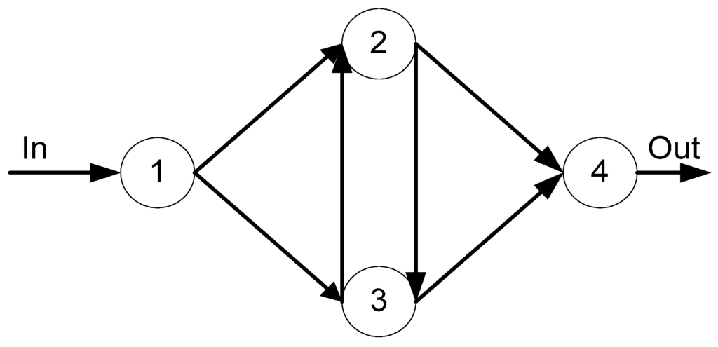
Figure 1.
A typical network flow diagram.
There are four basic properties associated with arc: cost coefficient c, flow efficiency η, lower bound emin, and upper bound emax. Other properties can also be represented, such as generators’ emission rate, ramp-up/ramp-down rates, start-up/shut-down costs, and transmission lines’ susceptance. The convex quadratic cost function of the arc flow can also be linearized by a piecewise linear function or a step function. Then a single arc can be substituted by multiple arcs, each representing one segment of the linear function. In the generation model, one generator is split into a pair of nodes so that operating constraints and variable operation and maintenance (O&M) costs can be expressed using the properties of the arc connecting the two nodes. A generator’s marginal cost is mainly determined by its fuel cost and variable O&M cost [20]. Both costs can be incorporated using the generalized network flow formulation.
In Figure 2, when the generator is bidding at its marginal costs, the three arcs represent the generator energy cost curves. As the objective of the production cost simulation problem is the minimization of total production cost, arc 1 will first be used to transfer the energy flow due to its low cost. When the demand increases and flow in arc 1 reaches its limit, arc 2 will then be used, followed by arc 3.
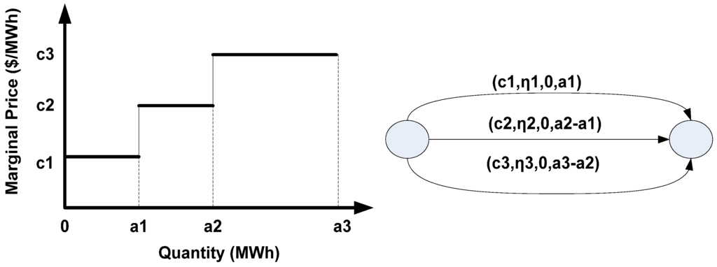
Figure 2.
A generator marginal cost curve.
2.2. Storage Model
The CAES is comprised of a compressor, a gas turbine/generator, and an air reservoir. In Figure 3, the three major components are represented by arcs L1, L2, and L3, respectively. At each time step, storage can buy electricity from the market, sell electricity to the market, or do nothing. Arc L4 represents the amount of energy purchased from the market at each time step. L5, on the other hand, represents the amount of the energy sold to the market. Separating the energy purchase and energy generation into two arcs enables the detailed modeling of the two processes.
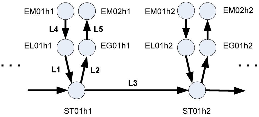
Figure 3.
Energy storage system model.
L1 models the operations of the compressor. The compressor capacity (L1max) is defined as the maximum amount of power that it can use to compress the air at each time step. The efficiency (ηL1) of the compressor is defined as the total stored energy divided by the total energy input. The O&M cost of the compressor can be modeled as the cost associated with the energy flow in L1.
L2 represents the process of converting the potential energy in the compressed air to electric energy. During this process, the compressed air is released to the combustor through a recuperator. Natural gas is also injected to the combustor to produce high temperature gases. The expanded high temperature gases are then transferred to the turbine, which converts the energy stored in gases into mechanical energy in the turbine shaft. The turbine is connected with a generator which converts mechanical energy to electric energy [21]. The fuel and O&M costs, efficiency, and minimum/maximum capacity of the gas turbine/generator can be considered by specifying the cost, efficiency, and minimum/maximum flow limit of the arc L2, respectively. At each time step, the energy output is limited by the maximum capacity of the gas turbine or the energy storage level in the air reservoir, whichever is less. As natural gas is added to the energy conversion process, the efficiency of L2, which is calculated as the total energy output divided by total potential energy of the consumed compressed air, is higher than 1.
L3 represents the storage level in the air reservoir. The energy flow in L3 is decided by L1, L2, and the storage level at the last time step. There is a loss factor associated with L3 to represent the leaks in the energy storage system over time.
Arcs L1, L2, and L3 represent the operating characteristics of various components of CAES; Arcs L4 and L5, on the other hand, describes the purchase and sale of CAES in the electricity market at each time step, respectively. From the market’s perspective, the CAES is represented as two nodes: EM01 and EM02. EM01 is considered as a load while EM02 is considered as a generator. Similar to the way generators’ incremental marginal cost curves are modeled, the decremental energy purchase bid curve of CAES can also be considered in L4. The various bidding strategies of CAES can be represented by modifying the properties of L4, which can be one or multiple arcs.
L5 models the CAES energy sale into the electricity market. As the energy market and the ancillary services market are co-optimized, L5 contains the energy, regulating reserve, spinning reserve, and non-spinning reserve biddings. Each kind of bidding is comprised of several arcs, which correspond to the segments of CAES bidding curve, as illustrated in Figure 2. For each node in Figure 3, the total energy that flows in must be equal to the total energy that flows out. As the cleared reserves in the market do not incur energy flow, the energy flow balance equation for node EM02 does not consider reserve biddings. Additional constraints are added to the production cost simulation problem to represent reserve-related limits, e.g., CAES can provide regulation/spinning reserves when it is online.
The CAES model does not prohibit the simultaneous operation of the compressor and the gas turbine as this operating scenario is feasible and necessary in reality [22]. For example, due to ramp rate constraints, it is sometimes economical to buy and sell in the same time (details are shown in the case study section).
Based on the ways in which a CAES system treats the heat in the compressed air, there are three types of air storage: adiabatic, diabatic, or isothermal. As of 2012, there is no utility scale adiabatic or isothermal storage units yet. An adiabatic storage project named ADELE, which aims to commercialize adiabatic CAES, is currently underway in Germany [23]. The only two commercial CAES units in the world, the McIntosh (McIntosh, AL, USA) CAES plant and the Huntorf (Huntorf, Germany) CAES plant, use diabatic storage [24]. The CAES model proposed above can capture the characteristics of diabatic CAES units. By removing the cost/efficiency associated with the gas turbine and considering the cost/efficiency of the adiabatic storage, the proposed CAES model can be applied to adiabatic CAES units as well.
3. Formulation of the Co-Optimization Problem
In order to evaluate the economic performance of CAES and its impacts on the operations of the electric system, a long-term production cost simulation model is built. In the production cost simulation model, an hourly day-ahead energy and ancillary services market and a 5-minute real-time market are considered. The co-optimization of the energy market subject to transmission constraints and the ancillary service market subject to resource constraints is implemented in both the day-ahead and real-time markets.
In the 5-minute RT market, the Independent System Operator (ISO) conducts the economic dispatch of the whole fleet of committed units every 5 minutes. There are several major differences between the DA market and RT market: (1) the DA market uses forecasted hourly wind/demand profiles, while the RT market uses actual 5-minute wind/demand profiles. The intra-hour fluctuations of wind and load affect the RT dispatch; (2) There are forced outages of generators and transmission lines in the RT market which are not considered in the DA market; (3) DA market simulates the operations of the system for the 24-hour period, while RT market determines the actual operations of the market at every 5-minute period. Additional constraints between two consecutive 5-minute periods, such as ramp rate limits, need to be included in RT simulation.
After the DA and RT markets are cleared, the total profits of CAES can be calculated as DA energy and reserve revenues + RT additional energy and reserve revenues or penalty costs – RT production costs. DA energy and reserve revenues are scheduled energy/reserve amount times their corresponding marginal prices. In the RT market settlement, if CAES provides more energy or reserves than DA schedules, the additional energy or reserves are priced at RT prices. If CAES provides less energy or reserves than DA schedules, CAES needs to pay for the differences at RT prices.
3.1. Wind/Load Profiles
In many previous studies, wind was modeled as negative load, which means it cannot be curtailed by the production cost simulation model [25,26]. In the recent years, in order to fully integrate wind into the energy market and reduce manual wind curtailment, some ISO/RTOs started to treat wind in a similar manner to the other resources. In this paper, wind units are modeled as dispatchable intermittent resource (DIR), which means wind units can actively bid in the energy market but are not eligible to supply operating reserves (regulating, spinning, or supplemental) [27].
Many attempts have been made to use statistical methods to model the wind power output variation. In this study, a nominal 1 MW multivariate wind power hourly production time series is used to represent the day-ahead forecast for each wind farm. The historical maximum wind output values were used in the real-time market simulation. The historical and forecasted wind outputs are obtained from the Eastern Wind Dataset created by AWS-Truewind and National Renewable Energy Laboratory (NREL) [28].This wind time series data considers geographic variations, model bias, turbine and plant availability, and other factors [29] and is widely used in many regional and inter-regional studies. The wind output at each time step is limited by wind farm maximum capacity times its time series value. As demand forecast techniques are very mature and have small forecast errors, the load forecasting uncertainty is not considered in this paper.
3.2. Unit Commitment Problem Formulation
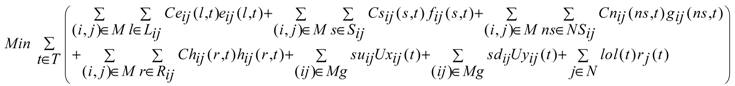
The unit commitment problem is formulated as a mixed-integer optimization problem. The objective function is the minimization of {energy costs + spinning reserve costs + non-spinning reserve costs + regulating reserve costs + start-up costs + shut-down costs + loss of load penalties}:
At each node, the sum of flow injections minus the sum of flow extractions equals the demand at that node:

Branch flow calculation:
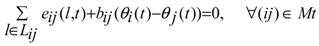
Flow constraints:
The sart-up and shut-down status of each generator:

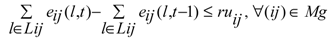
Up-ramp constraints:
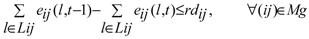
Down-ramp constraints:
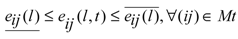
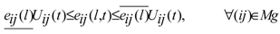
Constraints on generator ij energy bidding curve segments:
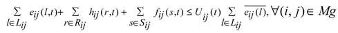
Constraints on generator ij energy and reserve bids:

Constraints on generator ij regulating reserve and spinning reserve bids:
System total operating reserve requirement:

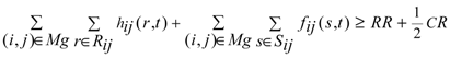
System total regulating and spinning reserve requirement:
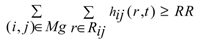
System total regulating reserve requirement:
CAES energy storage level at time t:

CAES energy and reserve bids constraint:

Wind generation output constraints:
The generator start-up and shut-down costs are considered in the objective function. In Equations (1) and (5), Ux and Uy are binary variables indicating whether unit ij is switched on or shut down at time t or not, respectively.
A generating unit has limited ability to vary its generation output from one time step to the next. The ramp-up and ramp-down constraints of each generator are defined in Equations (6) and (7), respectively.
If a unit is on-line, it can submit energy, regulating, and spinning reserves offers. If it is off-line, it can only bid non-spinning reserve. In both cases, the sum of three reserves needs to be constrained by the generator maximum capacity, as illustrated in constraint Equation (9). To ensure that the highest quality service is procured if economically appropriate, higher quality reserve (spinning reserve) can substitute for low quality reserve (non-spinning reserve). Constraints Equations (9) and (10) ensure that the ancillary service bids of a generator are constrained by its operating status and maximum capacity.
In order to ensure the reliable operation of the energy system, sufficient contingency reserve needs to be provided. Contingency reserve is defined as:
where CR1 is 5% of hydro generation +7% of generation provided by other conventional generators (excluding intermittent generation resources) +10% of wind power output; CR2 is the MW loss of generation due to the outage of the largest generating unit at each hour. Spinning reserve needs to be at least 50% of the operating reserve requirement. The reason that hydro generation requires less reserve than traditional generators is that non-hydro generation has higher risks related to fuel scheduling and forced outages. With exception of the wind power component, this definition of operating reserve is consistent with California ISO’s contingency reserve requirement [30]. Current contingency reserve definitions do not include an explicit wind power component as we do here. However, as many studies point out, with the increase in wind penetration level, more reserves are needed to back up wind fluctuations [31,32].
CR = max {CR1,CR2} + 100% of non-firm imports
As shown in Figure 3, from the market’s perspective, the CAES is modeled as one generator node and one load node. The constraints associated with those two nodes are already captured in Equations (1–13). Equations (14) and (15) represent constraints associated with the stored energy in CAES, which are not captured in previous functions.
Equation (14) calculates the storage level of CAES. At the end of time t, the energy stored in the air reservoir is decided by the storage level at previous time step times the storage reservoir loss factor, purchased energy at time t times the compressor efficiency, and total stored energy used by the gas turbine at time t. Equation (14) describes the energy balance at node ST01 in Figure 3.
Equation (15) describes the impact of total stored energy on the energy and reserve bids. The total amount of energy + ancillary services must be limited by the total stored energy in the air reservoir.
3.3. Hourly Economic Dispatch Problem Formulation
Based on the commitment schedule generated by the UC problem, the ED problem dispatches the committed units in the minimal cost way and obtains LMPs at each node for energy and market clearing prices (MCP) for ancillary services. As the result of the co-optimization of the energy and ancillary services markets, the reserve prices will reflect the marginal costs of the services as well as the lost opportunity costs incurred by having to back up rather than bidding in the energy market.
The ED problem is similar to the UC problem, except that uij is a parameter rather than a variable in the ED formulation. The start-up and shut-down costs are fixed after the unit commitment schedule is decided so they are not considered in the objective function of the ED problem.
3.4. Sub-Hourly Economic Dispatch Problem Formulation
In order to simulate the real-time market operations, a 5-minute economic dispatch model is formulated. DA hourly reserve requirements are used in the 5-minute simulation. Different from the wind/load profiles used in DA simulation, the 5-minute historical synchronous wind and load profiles is used. Figure 4 shows the forecasted wind and actual wind of a typical wind farm using the Eastern Wind Dataset. Compared with DA hourly wind forecast, the actual wind output has higher variations and the magnitude/time of the maximum/minimum output might be different, which requires enough flexible generation available to accommodate the forecast errors in the RT market.
Besides wind and demand profiles, another major difference between our modeled hourly dispatch and sub-hourly dispatch is the ramping requirement. Compared with hourly simulation which has hour-to-hour ramp requirements, the RT simulation has ramp constraints on generation output for every 5 min. As wind output fluctuates in the sub-hourly timeframe, base load units sometimes cannot ramp quickly enough to meet the demand, which requires fast maneuverable generation units, such as CAES, to be dispatched.
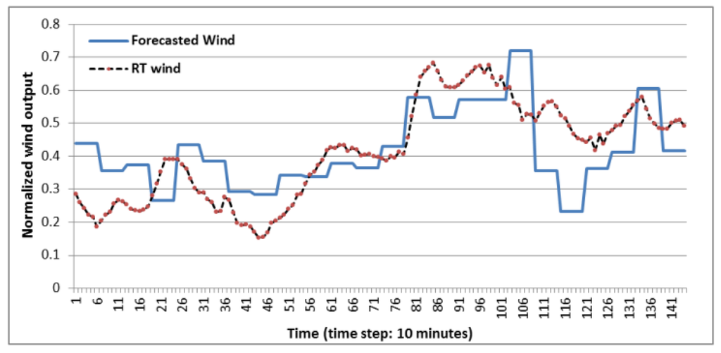
Figure 4.
Forecasted wind vs. actual wind.
4. Case Study
The proposed methodology is implemented using MATLAB, TOMLAB and CPLEX and is applied on a modified IEEE 24-bus reliability test system (RTS) [33], as shown in Figure 5. The flow constraints of each transmission line are reduced by 50%. No imports/exports from/to external systems are considered.
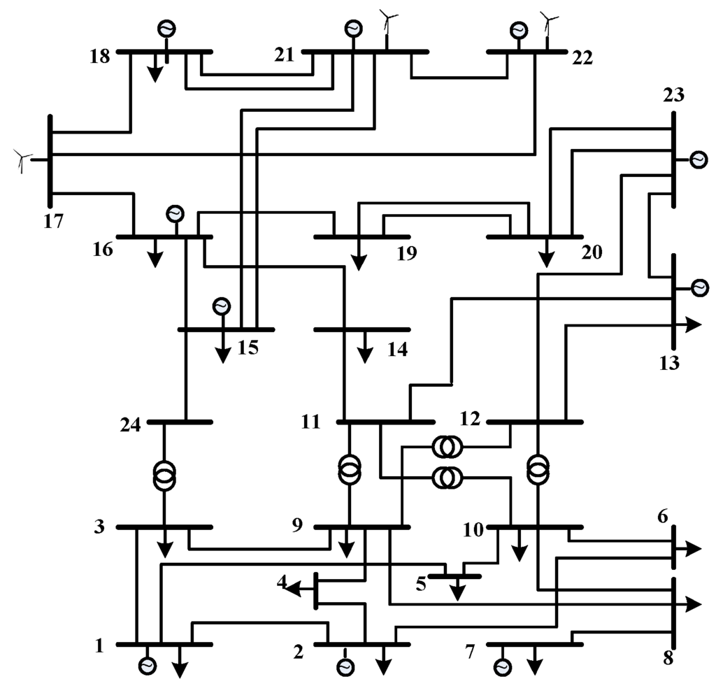
Figure 5.
IEEE 24-bus reliability test system.
Three wind farms with 300 MW, 400 MW, and 300 MW capacity are located at buses 17, 21, and 22, respectively. The capacity factors for the three wind farms are 30%, 35%, and 30%. In this way, the 20% wind penetration level is reached. Hourly forecasted and 5-minute historical synchronously recorded wind power output data at each wind site is used. All wind generators are located in the upper part of the system while the load center is in the lower part. Three sets of 1-MW wind time series data (historical wind data and forecasted wind data) in western MISO region are randomly selected from the Eastern Wind Dataset. The three RT actual wind time series data are scaled up or down to match the capacity factors of the three wind farms, respectively. The DA forecasted wind time series data are then multiplied by their corresponding scaling factors (wind farm’s capacity factor divided by the average value of RT actual wind time series). The hourly load profiles are obtained from the 24-bus test system. The load forecasting errors are not considered, so the RT 5-minute profiles are created by linearly interpolating the hourly values. The demand is considered as inelastic.
For each generator, the heat-rate values at different generation output segments are obtained from the 24-bus test system. In order to represent the up-to-date values of fuel costs, the fuel costs used in this study are updated based on the latest MISO Transmission Expansion Plan (MTEP) model in 2012 [34]. The MTEP model was created based on public available information and MISO stakeholder inputs and vetted by the MISO stakeholders. The fuel prices used in this study are shown in Table 1 below.

Table 1.
Fuel prices.
| Fuel Type | Gas | Oil | Coal | Uranium |
|---|---|---|---|---|
| Fuel Price ($/MMBTU) | 4.25 | 19.4 | 2.5 | 1.14 |
The original 24-bus test system has many oil-burning units, partially due to the low oil prices in 1970s, when the test system was created. As the oil price has increased significantly since then, most oil-burning units were either retired or converted to natural gas-fired technology. Currently, only about 4% of total nameplate capacity in the Eastern Interconnection burns oil [34]. In order to make sure the test system is realistic; eleven out of the fifteen oil-fired units in the test system are switched to natural gas-fired units. Only the four 20 MW units remain unchanged. The six hydro units (50 MW) are switched to coal units as well. The modified test system has 4455 MW total nameplate capacity. Table 2 below shows the resource mix of the modified test system.
Table 2.
Resource mix.
| Power Plant Type | Oil | Coal | Nuclear | Gas | Wind |
|---|---|---|---|---|---|
| Nameplate Capacity (MW) | 80 | 1574 | 800 | 951 | 1000 |
The input parameters of the CAES unit are shown in Table 3 below. CAES operates on a daily cycle, i.e., charge in off-peak hours and discharge in peak hours on a daily basis. The operation of the system is simulated for one typical winter week and one typical summer week.
Table 3.
Input data for cases.
| CAES Plant | Compressor capacity = 50 MW |
| Compressor efficiency = 70% | |
| Compressor variable O&M cost = 2.0 $/MWh | |
| Storage capacity = 200 MWh | |
| Storage self-discharge rate = 1% | |
| Turbine capacity = 50 MW | |
| Turbine efficiency = 200% | |
| Turbine heat rate = 4.0 MMBTU/MWh | |
| Turbine variable O&M cost = 2.0 $/MWh | |
| Natural gas price = 4.25 $/MMBTU |
This CAES unit represents the state-of-the-art technology. The compressor efficiency is obtained from [5]. The O&M costs of compressor and gas turbine are based on general operating characteristics of compressor and gas turbine [3]. The turbine heat rate is obtained from [3]. The turbine efficiency is defined as the total turbine output divided by the total compressed air energy input. Since the consumed natural gas is not considered in this calculation, the turbine efficiency is more than 100% [5].
Many studies have been made to evaluate the optimal siting strategy of CAES. A case study in ERCOT demonstrates that the economically optimal location for the CAES is close to load center [35]. Another study in NY, however, shows that the optimal location of the CAES in New York transmission system would be “as close as possible to a large wind resource, if transmission constraints are not an issue” [36]. In this study, two scenarios are considered when evaluating the economic performance of CAES:
- (1)
- A CAES is sited at bus 21, which is near the wind sites and far away from the load center;
- (2)
- A CAES is sited at bus 2, which is remote from the wind sites and close to the load center.
The performance of CAES in DA and RT markets under scenario 1 is shown in Figure 6 and Figure 7, respectively. The simulation results of a summer day are used in the two figures. In the CAES charge curve, positive value means the CAES is charging (buying electric power from the market), while in the CAES discharge curve, negative value means the CAES is discharging (selling electric power to the market). The hourly and 5-minute LMPs at bus 21 are also included in Figure 6 and Figure 7, respectively.
The optimization model evaluates the system operating conditions and determines whether CAES should charge, discharge, or do nothing. The charge/discharge patterns and potential energy arbitrage revenue of CAES are mainly affected by the fluctuations of the LMPs at the bus where CAES is located. As there is plenty of generation capacity in the upper region and the transmission lines between the two regions are congested almost all the time, low-cost energy is continuously available in the upper region and the spread between off- and on-peak prices is relatively small. Consequently, there is not too much opportunity for CAES to perform energy arbitrage in the DA market.
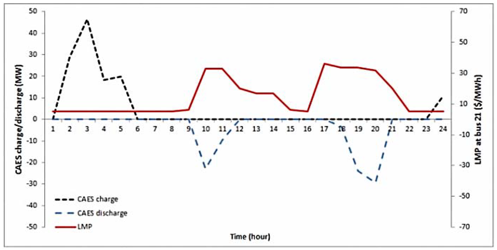
Figure 6.
CAES DA charge/discharge schedule and DA LMPs at bus 21 under scenario 1.
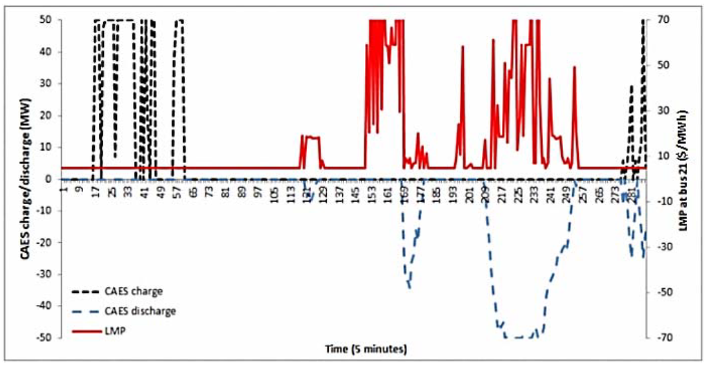
Figure 7.
CAES RT charge/discharge values and RT LMPs at bus 21 under scenario 1.
In the RT market, however, the actual LMP profile is more volatile than the DA LMP profile because of the intra-hour wind fluctuations and DA wind forecast errors. Compared with the peak DA LMP, the peak RT LMP is higher in magnitude and occurs at a different time, which results in different RT CAES discharge schedule. By comparing Figure 6 and Figure 7, it can be found that the DA-only simulation cannot fully capture the revenues of CAES; the actual revenue of CAES can be quite different from the DA market.
In Figure 7, the CAES does not discharge during time 153–169, when the LMPs are high. This seems counterintuitive; however, the production cost problem optimizes the generation dispatch to minimize the total system energy + reserve costs. It is possible that holding CAES’s generation during that time period might be more economical for the total system.
Figure 8 and Figure 9 show the DA and RT operations of the CAES under scenario 2 in a summer day. In the lower region, the LMP fluctuations are much higher than those in the upper region as the result of congestions in the system, high demand, and high marginal costs of generators in that region. In the off-peak hours, the transmission lines between the two regions are less congested and wind farms have high output, so low-cost wind energy are transferred to the lower region and stored in the CAES. In the peak hours, as the result of limited transmission capacity connecting the two regions, there are significant congestions in the transmission system, which cause the dispatch of high-cost units in the lower region and higher LMPs. The high-penetration of wind increases the spread of off- and on-peak prices, so the profitability of the CAES is enhanced. In this scenario, besides performing energy arbitrage, CAES also helps to relieve the transmission bottlenecks as energy can be transferred from the upper region to the lower region during the off-peak hours when there is less congestion in the system. Compared with DA schedule, CAES is also more active in the RT market.
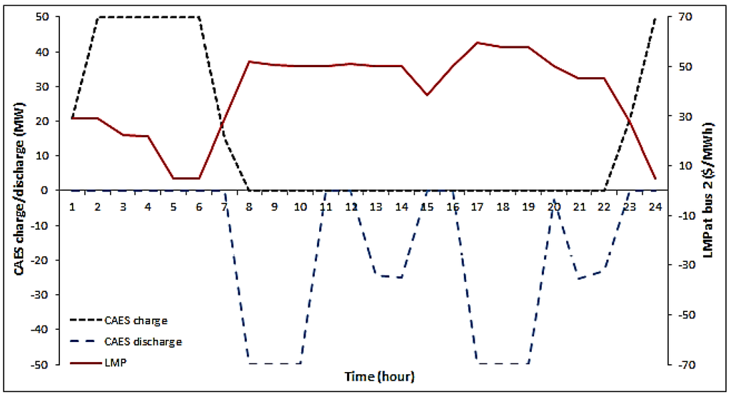
Figure 8.
CAES DA charge/discharge schedule and DA LMPs at bus 2 under scenario 2.
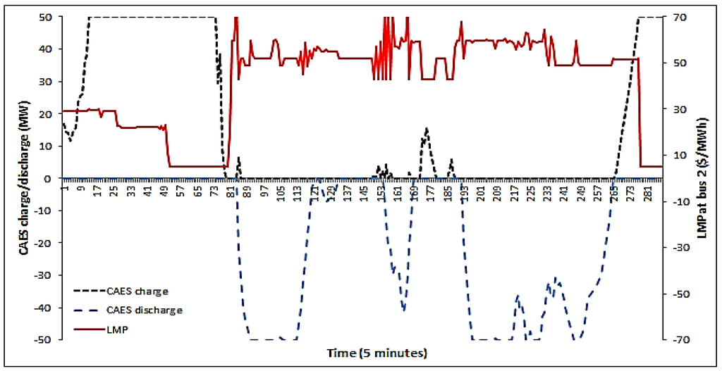
Figure 9.
CAES RT charge/discharge values and RT LMPs at bus 2 under scenario 2.
As shown in Figure 7, Figure 8 and Figure 9, CAES charges and discharges simultaneously during some time intervals. If the ramp-up and ramp-down constraints of CAES gas turbine and the ancillary services market were not considered, the optimization problem would make sure that CAES does not charge and discharge simultaneously. In the proposed model, however, occasionally it might be more economical from the whole system’s perspective to charge and discharge CAES at the same time. For example, if there are low LMP price and high regulating/spinning reserve price at time t; the additional benefits gained from the reserve market are higher than the financial loss as the result of discharging at a low LMP. In this situation, the optimization model will charge and discharge CAES to minimize total system costs. Since the charging process is done by the compressor of the CAES and the discharging process is done by the gas turbine, the simultaneous charging and discharging can be performed physically.
Besides providing electric energy, CAES can also provide high-value ancillary services. Figure 10 shows the CAES profits from the energy and ancillary services markets. All profits are calculated based on both DA and RT market dispatch results. As shown in Figure 10, CAES can gain a significant amount of profits from the ancillary service market under both scenarios. Under scenario 1, where CAES is located near the wind sites, CAES gained limited profits from the energy market but received high profits from the ancillary services market. Under scenario 2, however, the main source of CAES’ profits comes from energy market. As illustrated in Figure 10, the CAES can gain more annual profits under scenario 2 (close to the load center).
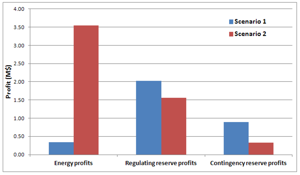
Figure 10.
Annual profits of CAES.
A sensitivity analysis was conducted to evaluate the effects of CAES capacity on its annual earning and total system production cost under scenario 2. In Figure 11, the CAES profits first go up and then go down as CAES capacity increases. When the CAES capacity is doubled or tripled, it can get more profits by providing energy and ancillary services. However, as the CAES is bidding at its marginal cost, when CAES capacity gets larger and larger, it displaces the high cost units during the peak hours, resulting in lower peak hour prices and smaller gap between on-peak and off-peak prices. As the CAES is paid the LMP for its energy, it will have less revenue. When the CAES capacity is infinite, it will totally displace the high-cost peak generators resulting in a flat LMP profile. As the energy arbitrage profits of CAES are dependent upon the LMP fluctuations, CAES realizes limited profits when it has infinite capacity. The ancillary services prices are mainly determined by the opportunity costs of backing up the generation rather than selling in the energy market. When the system has flat LMP profile, the opportunity costs of the reserves are very low, which results in low ancillary services profits.
As shown in Figure 11, the CAES’s profits do not grow proportionally to the facility capacity. This implies there is an optimal CAES capacity with the highest benefit-cost (profits-investment cost) ratio for each system. As strategic bidding is not considered in this study, which means that the CAES always bids at its marginal costs and makes all of its capacity available to the system, the actual profits of the CAES in reality could be higher.
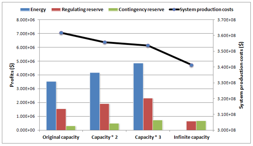
Figure 11.
CAES annual profits and system total production costs vs. CAES capacity.
Although the CAES’s profits first rise and then fall with increasing capacity, the system total production cost continuously decreases with increasing CAES capacity. This is because the economic dispatch problem optimizes the system generation dispatch rather than CAES profits, which results in lower system production cost and lower system LMPs.
Note that since an objective of the paper is to introduce the mathematical optimization model as well as the detailed CAES model, the case study focuses on evaluating the economic performance of CAES in the market rather than assessing whether it is economical to build CAES or not. The life-cycle economic analysis of CAES, however, can be performed using the proposed model, given information such as investment cost, construction lead time, etc.
To study the performance of CAES in a transmission-constrained system, the transmission thermal limits are reduced in the case study. In actual systems, the ISOs might consider investing transmission lines to relieve the congestion. The trade-off between building energy storage systems and building transmission lines to enhance system operating efficiency and relieve congestion is an interesting topic and will be explored in our further work.
5. Conclusions
In this paper, a mathematical optimization model of the electric power system was developed to assess the economic value of CAES. The operations of the DA and RT energy market and ancillary services market were co-optimized to quantify the benefits of CAES, such as load leveling, peak shifting, and providing high-value regulating, spinning and non-spinning reserves. A detailed model of CAES was also proposed, which considered the costs, efficiencies, and capacities of the compressor, the gas turbine/generator, and the air reservoir.
The proposed production cost simulation model and CAES model were applied on a test system. The results demonstrate that: (1) besides profits from the energy arbitrage, CAES could also get significant profits by providing high quality reserves in the ancillary services market; (2) CAES can take advantage of the wind/load forecast errors and wind intra-hour fluctuations and gain additional profits in the RT market; (3) The siting and sizing of CAES will drastically affect the profitability of CAES as the result of transmission congestions. By including a detailed CAES model and simulating the DA and RT co-optimized energy and ancillary services market, the proposed can capture all of the aforementioned value streams.
Nomenclature
| Sets | |
| T | Set of time periods |
| M | Set of arcs |
| Mg | Set of arcs representing power generation processes for generators (excluding wind farms) |
| Mt | Set of arcs representing electric transmission system |
| N | Set of nodes |
| Ng | Set of generators (excluding wind farms) |
| Nc | Set of air compressors |
| Nt | Set of buses in the transmission system |
| Nw | Set of wind farms |
| Ns | Set of compressed air energy storage units |
| Lij | Set of linearization segments of the energy bid in arc ij |
| Rij | Set of linearization segments of the regulating reserve bid in arc ij |
| Sij | Set of linearization segments of the spinning reserve bid in arc ij |
| NSij | Set of linearization segments of the non-spinning reserve bid in arc ij |
| Variables | |
| eij(l,t) | Energy flow segment l in arc ij during period t |
| hij(r,t) | Regulating reserve bid segment r in arc ij during period t |
| fij(s,t) | Spinning reserve bid segment s in arc ij during period t |
| gij(ns,t) | Non-spinning reserve bid segment ns in arc ij during period t |
| Uij | Unit commitment decision variable for generator ij |
| ri(t) | Load curtailment at node i during period t |
| θi | Phase angle of bus i |
| Parameters | |
| Ceij(l,t) | Per-unit cost of the energy flow segment l in arc ij during period t |
| Chij(r,t) | Per-unit cost of the regulating reserve bid segment r in arc ij during period t |
| Csij(s,t) | Per-unit cost of the spinning reserve bid segment s in arc ij during period t |
| Cnij(ns,t) | Per-unit cost of the non-spinning reserve bid segment ns in arc ij during period t |
 | Upper bound on the energy flow in arc ij |
 | Lower bound on the energy flow in arc ij |
| ηij | Efficiency parameter associated with the arc ij |
| ηii | Efficiency parameter associated with the arc connecting CAES i from one time step to the next |
| lol | Load curtailment penalty cost |
| bij | Susceptance of the arc ij |
| δ(t) | System wind penetration level during period t |
| σij | Capacity factor for wind farm ij |
| woij(t) | Nominal 1-MW wind power time series ij during period t |
| dj(t) | Supply (if positive) or demand (if negative) at node j, during period t |
| ruij | Generator ij’s up-ramp rate limit |
| rdij | Generator ij’s down-ramp rate limit |
| suij | Generator ij’s start-up cost |
| sdij | Generator ij’s shut-down cost |
| uij | Unit commitment decision for generator ij (this is the value of Uij, not a variable) |
| Acronyms | |
| ESS | Energy storage system |
| CAES | Compressed air energy storage |
| DA | Day-ahead |
| RT | Real-time |
| O&M | Operation and maintenance |
| LMP | Locational marginal price |
| MCP | Market clearing price |
| UC | Unit commitment |
| ED | Economic dispatch Independent |
| ISO | Independent System Operator |
| MISO | Midwest Independent Transmission System Operator |
| MTEP | MISO Transmission Expansion Plan |
Conflict of Interest
The authors declare no conflict of interest.
References
- U.S. Department of Energy. 20% Wind Energy by 2030—Increasing Wind Energy’s Contribution to U.S. Electricity Supply; U.S. Department of Energy: Washington, DC, USA, 2008. [Google Scholar]
- Benitez, L.E.; Benitez, P.C.; van Kooten, G.C. The economics of wind power with energy storage. Energy Econ. 2008, 30, 1973–1989. [Google Scholar] [CrossRef]
- Denholm, P.; Sioshansi, R. The value of compressed air energy storage with wind in transmission-constrained electric power systems. Energy Policy 2009, 37, 3149–3158. [Google Scholar] [CrossRef]
- Denholm, P.; Ela, E.; Kirby, B.; Milligan, M. The Role of Energy Storage with Renewable Electricity Generation; Technical Report, NREL/TP-6A2–47187; National Renewable Energy Laboratory: Golden, CO, USA, 2010. [Google Scholar]
- Lund, H.; Salgi, G. The role of compressed air energy storage in future sustainable energy systems. Energy Convers. Manag. 2009, 50, 1172–1179. [Google Scholar] [CrossRef]
- Konrad, J.; Carriveau, R.; Davison, M.; Simpson, F.; Ting, D. Geological compressed air energy storage as an enabling technology for renewable energy in Ontario, Canada. Int. J. Environ. Stud. 2012, 69, 350–359. [Google Scholar] [CrossRef]
- Ibrahim, H.; Ilinca, A.; Perron, J. Energy storage systems-characteristics and comparisons. Renew. Sustain. Energy Rev. 2008, 12, 1221–1250. [Google Scholar] [CrossRef]
- Black, M.; Strbac, G. Value of bulk energy storage for managing wind power fluctuations. IEEE Trans. Energy Convers. 2007, 22, 197–205. [Google Scholar] [CrossRef]
- Energy Storage—Packing Some Power. The Economist. 3 March 2012. Available online: http://www.economist.com/node/21548495 (accessed on 18 April 2013).
- Makarov, Y.V.; Nyeng, P.; Yang, B.; Ma, J.; DeSteese, J.D.; Hammerstrom, D.J.; Lu, S.; Viswanathan, V.V.; Miller, C.H. Wide-Area Energy Storage and Management System to Balance Intermittent Resources in the Booneville Power Administration and California ISO Control Areas. Technical Report; Pacific Northwest National Laboratory: Richland, WA, USA, June 2008. Available online: http://www.pnl.gov/main/publications/external/technical_reports/PNNL-17574.pdf (accessed on 1 January 2013). [Google Scholar]
- Succar, S.; Williams, R. Compressed Air Energy Storage: Theory, Operation, and Applications; Energy Systems Analysis Group, Princeton Environmental Institute, Princeton University: Princeton, NJ, USA, 2008. [Google Scholar]
- Drury, E.; Denholm, P.; Sioshansi, R. The value of compressed air energy storage in energy and reserve markets. Energy 2011, 36, 4959–4973. [Google Scholar] [CrossRef]
- Das, T.; Krishnan, V.; Gu, Y.; McCalley, J.D. Compressed Air Energy Storage: State Space Modeling and Performance Analysis. In Proceedings of the 2011 IEEE Power and Energy Society General Meeting, Detroit, MI, USA, 24–28 July 2011; pp. 1–8.
- Hobson, E.; Fletcher, D.L.; Stadlin, W.O. Network flow linear programming techniques and their application to fuel scheduling and contingency analysis. IEEE Trans. Power App. Syst. 1984, PAS-103, 1684–1691. [Google Scholar]
- Lee, T.H.; Thorne, D.H.; Hill, E.F. A transportation model for economic dispatch-application and comparison. IEEE Trans. Power App. Syst. 1980, PAS-99, 2373–2382. [Google Scholar]
- Pang, C.K.; Wood, A.J. Multi-area generation system reliability calculations. IEEE Trans. Power App. Syst. 1975, PAS-94, 508–517. [Google Scholar]
- Gu, Y.; McCalley, J. Market-Based Transmission Expansion Planning. In Proceedings of the IEEE PES Power Systems Conference & Exhibition (PSCE), Phoenix, AZ, USA, 20–23 March 2011; pp. 1–9.
- Gu, Y.; McCalley, J.; Ni, M. Coordinating large-scale wind integration and transmission planning. IEEE Trans. Sustain. Energy 2012, 3, 652–659. [Google Scholar] [CrossRef]
- Edmonds, J.; Karp, R.M. Theoretical improvements in algorithmic efficiency for network flow problems. J. ACM 1972, 19, 248–264. [Google Scholar] [CrossRef]
- PJM Interconnection. Variable Operations and Maintenance (VOM) Costs: Educational Document. Available online: http://www.pjm.com/~/media/committees-groups/subcommittees/cds/20110321/20110321-item-04b-educational-paper-for-vom.ashx (accessed on 21 February 2013).
- Peter, V.; Weiner, D. Compressed air energy storage. Modern Power Syst. 1988, 8, 1–12. [Google Scholar]
- Lund, H.; Salgi, G.; Elmegaard, B.; Andersen, A.N. Optimal operation strategies of compressed air energy storage (CAES) on electricity spot markets with fluctuating prices. Appl. Therm. Eng. 2009, 29, 799–806. [Google Scholar] [CrossRef]
- ADELE—Adiabatic Compressed-Air Energy Storage (CAES) for Electricity Supply. Available online: http://www.rwe.com/web/cms/en/365478/rwe/innovation/projects-technologies/energy-storage/project-adele/ (accessed on 21 February 2013).
- Crotogino, F.; Mohmeyer, K.U.; Scharf, R. Huntorf CAES: More Than 20 Years of Successful Operation. In Proceedings of the Solution Mining Research Institute Meeting, Orlando, FL, USA, 23–25 April 2001.
- MISO. Midwest ISO Transmission Expansion Plan 2010; MISO: Carmel, IN, USA, 2011. [Google Scholar]
- Eastern Wind Integration and Transmission Study; National Renewable Energy Laboratory: Golden, CO, USA, February 2011.
- MISO Market Subcommittee. Dispatchable Intermittent Resource Implementation Guide; MISO: Carmel, IN, USA, 2011; Available online: https://www.midwestiso.org/Library/Repository/Meeting%20Material/Stakeholder/MSC/2011/20110301/20110301%20MSC%20Item%2012a%20DIR%20Implementation%20Update.pdf (accessed on 1 January 2013).
- Eastern Wind Dataset. Available online: http://www.nrel.gov/electricity/transmission/eastern_wind_methodology.html (accessed on 1 January 2013).
- Brower, M. Development of Eastern Regional Wind Resource and Wind Plant Output Datasets; National Renewable Energy Laboratory: Golden, CO, USA, 2009. [Google Scholar]
- California ISO. Spinning Reserve and Non-Spinning Reserve. Available online: http://www.caiso.com/docs/2003/09/08/2003090815135425649.pdf (accessed on 1 January 2013).
- Doherty, R.; O’Malley, M. A new approach to quantify reserve demand in systems with significant installed wind capacity. IEEE Trans. Power Syst. 2005, 20, 587–595. [Google Scholar] [CrossRef]
- Dany, G. Power Reserve in Interconnected Systems with High Wind Power Production. In Proceedings of the IEEE Porto Power Tech Conference, Porto, Portugal, 10–13 September 2011; pp. 6–11.
- Subcommittee, P.M. IEEE reliability test system. IEEE Trans. Power App. Syst. 1979, PAS-98, 2047–2054. [Google Scholar]
- MISO. MISO Transmission Expansion Plan 2012; MISO: Carmel, IN, USA, 2012. [Google Scholar]
- Fertig, E.; Apt, J. Economics of compressed air energy storage to integrate wind power: A case study in ERCOT. Energy Policy 2011, 39, 2330–2342. [Google Scholar] [CrossRef]
- New York State Energy Research and Development Authority. Compressed Air Energy Storage Engineering and Economic Study, Final Report; New York State Energy Research and Development Authority: Albany, NY, USA, 2009. [Google Scholar]
© 2013 by the authors; licensee MDPI, Basel, Switzerland. This article is an open access article distributed under the terms and conditions of the Creative Commons Attribution license (http://creativecommons.org/licenses/by/3.0/).