A New Two-Stage Approach to Short Term Electrical Load Forecasting

Abstract
:
1. Introduction
2. Least Squares Support Vector Machines Model
 and outputs
  . The following regression model can be built by using a non-linear mapping function
  which maps the input space into a high-dimensional feature space and constructs a linear regression in it. The regression model in primal weight space is expressed as follows:


 ,
,  ,
,  there are Lagrange multipliers, I is an identity matrix and
  denotes the kernel matrix.
 is known as a kernel function. Kernel functions that satisfy Mercer’s condition enable computation of the dot product in a high-dimensional feature space by using data inputs from the original space, without explicitly computing φ(x).
3. Model Formation
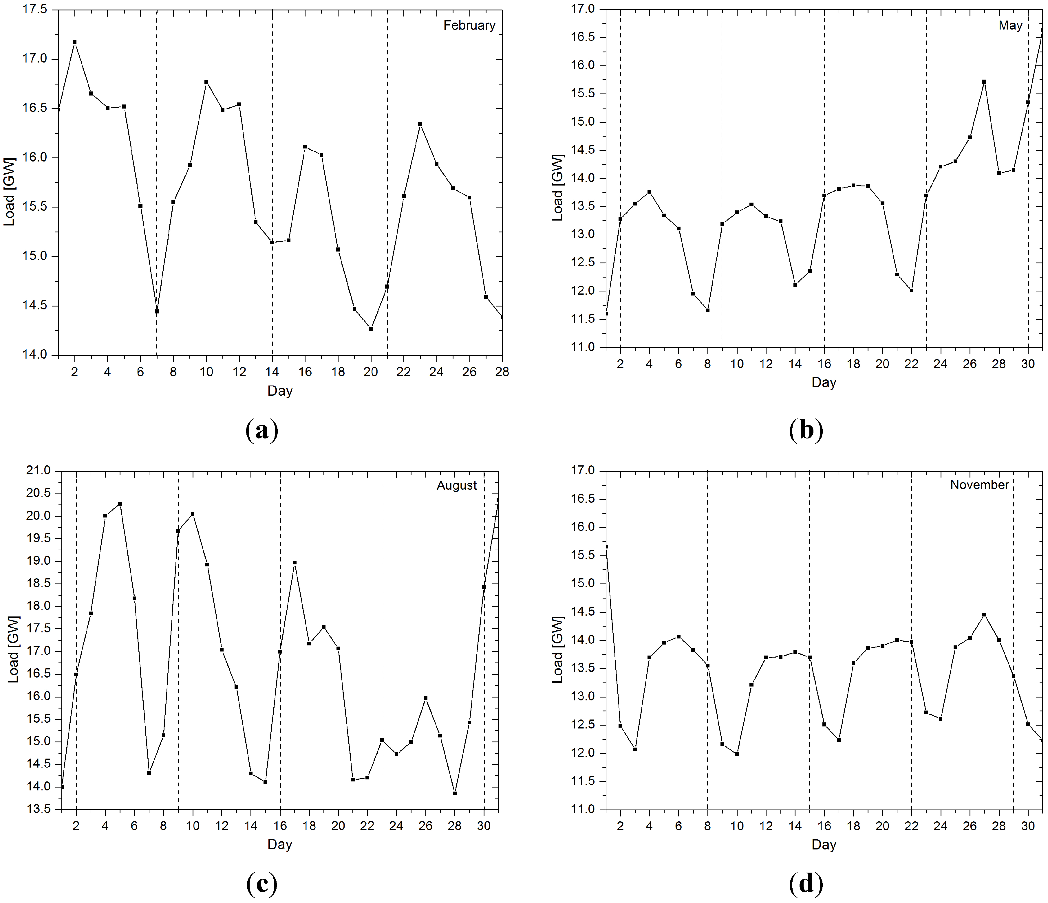
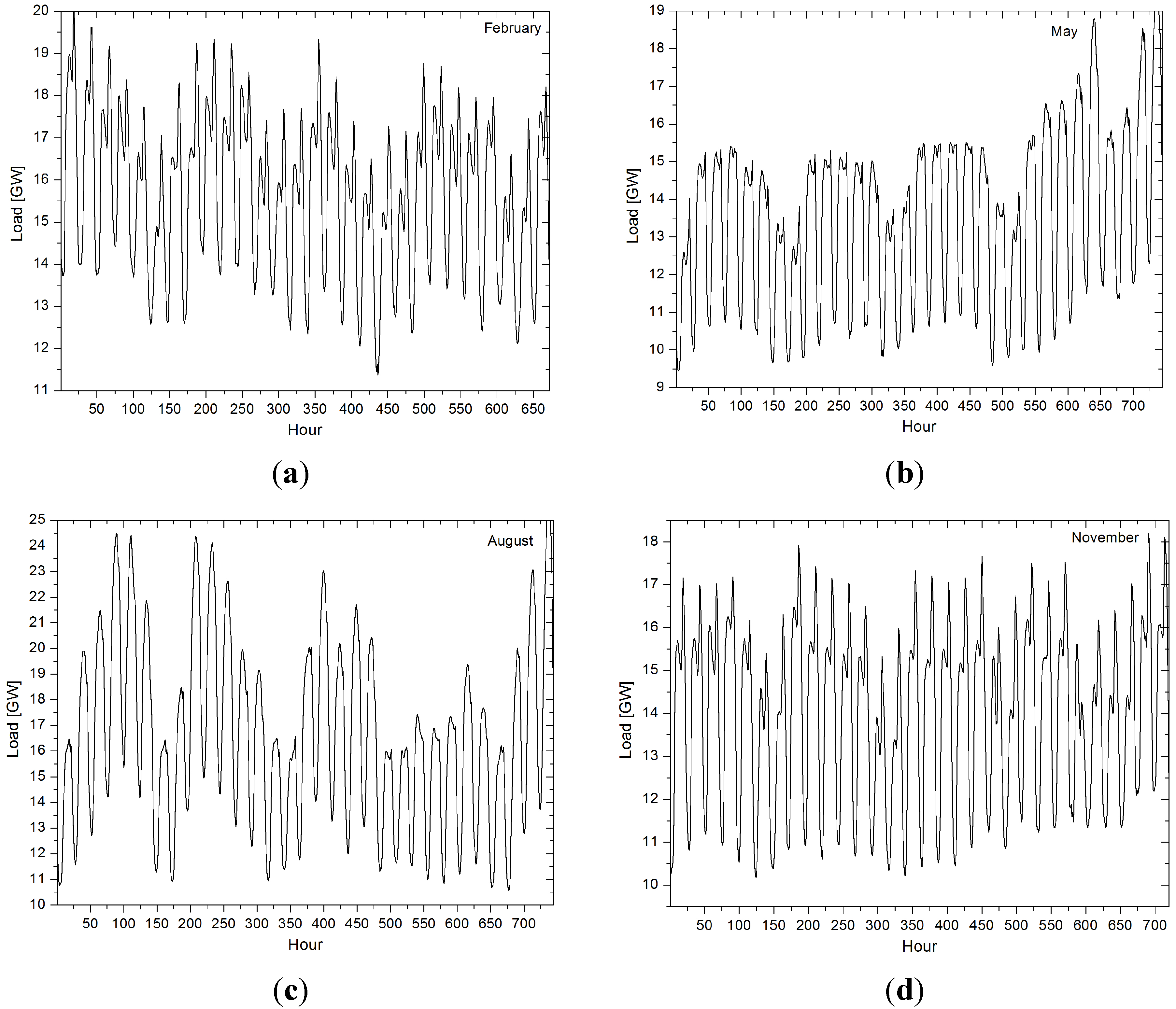
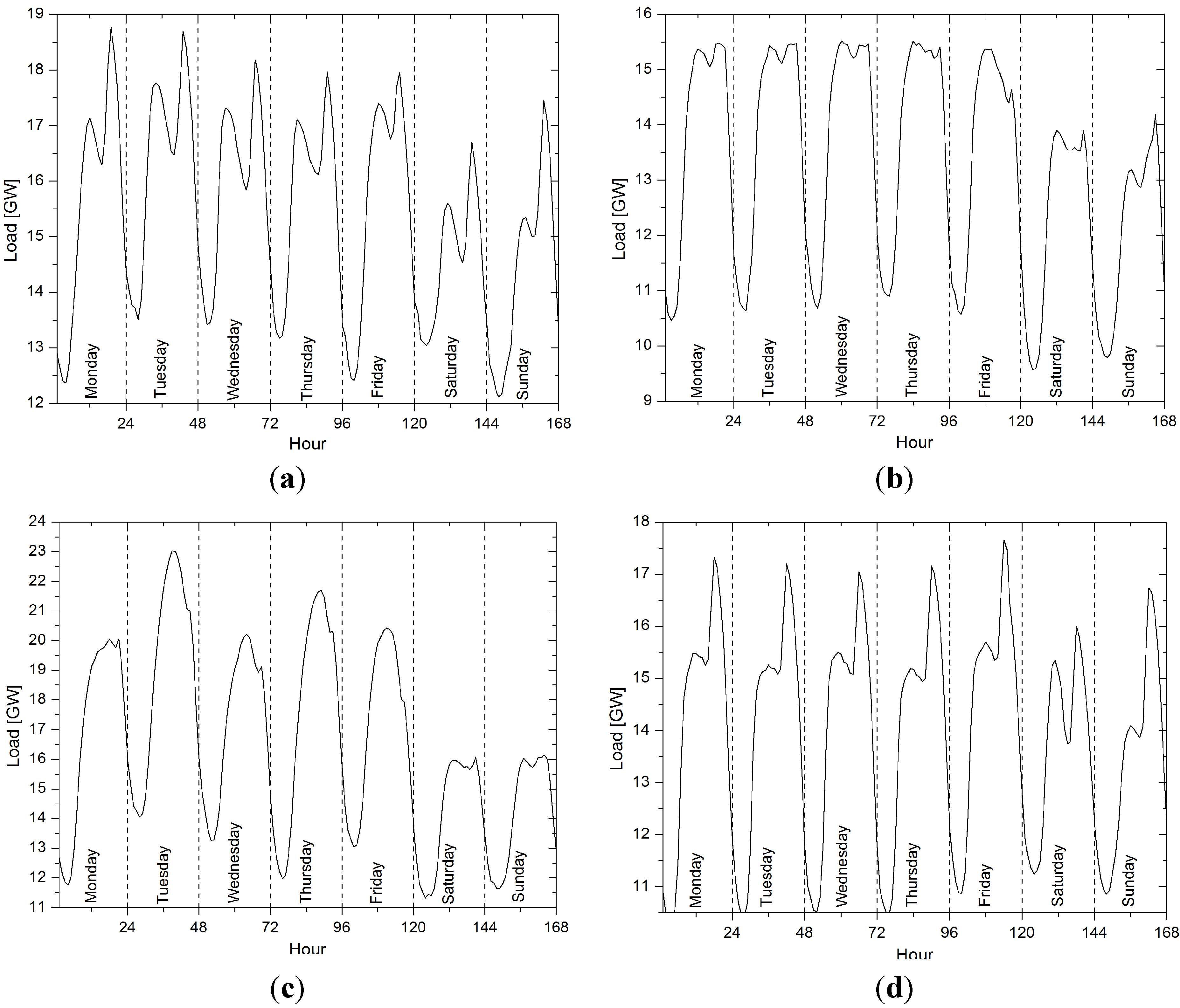
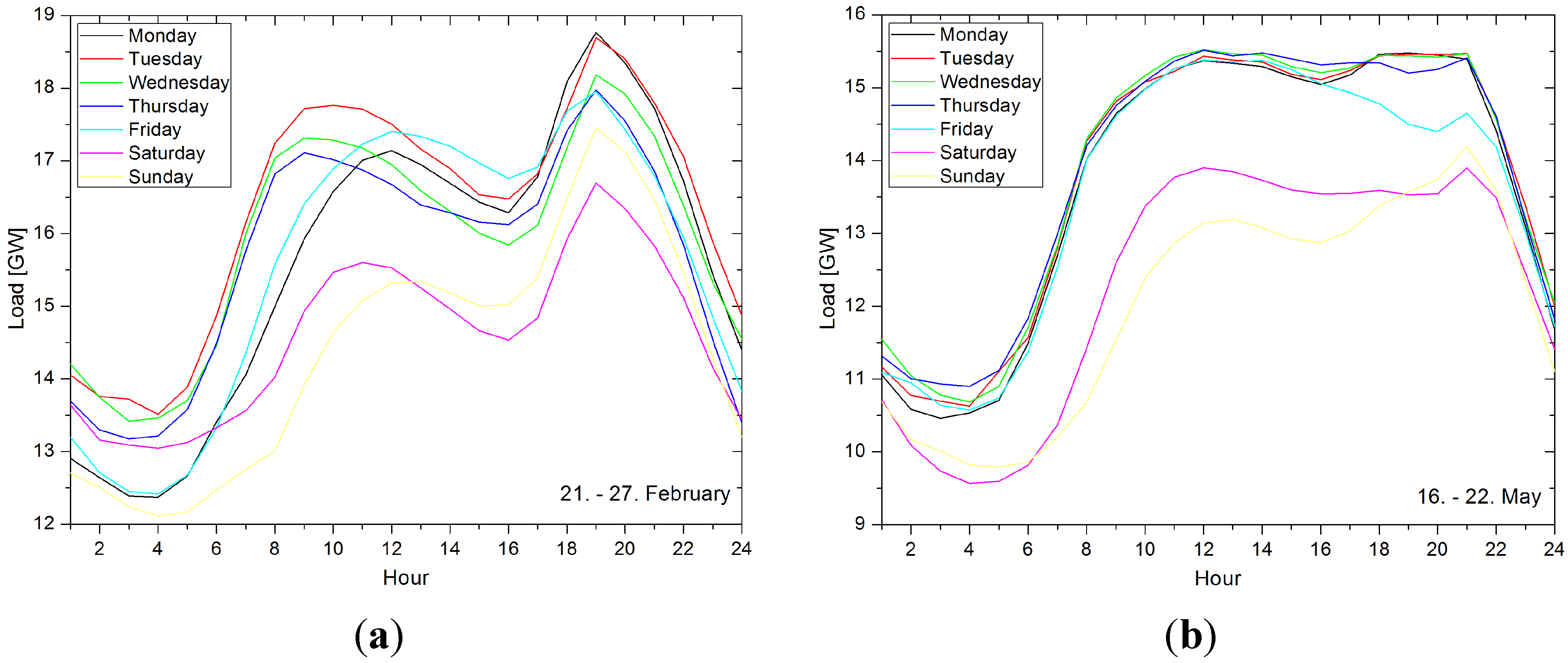
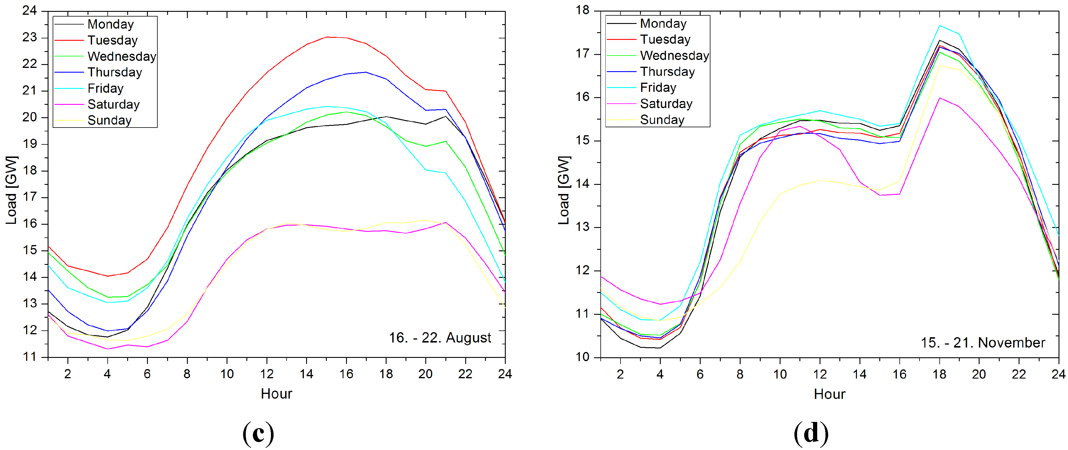
3.1. Features of Electric Load


3.2. The Proposed Approach
 , i = 1,…,7). To map the weekly load behavior, the day of the week feature (
  ,
,  where 1 corresponds to Monday, 2 to Tuesday and so on) is included in the feature set and this feature is the only non-time series feature, i.e., s = 1.
- 1.
- Stage I
- 1.1.
- Model I training set formation using daily average load data for the past three years. This training set contains 1095 vectors in total and each vector is composed of features from seven past average daily loads and the current day of the week indicator. Normalize all of the features in the [0–1] range by using min-max normalization,
- 1.2.
- Based on this training set and grid-search algorithm with a k-fold cross validation procedure (k = 10), obtain the optimal parameters γ and σ for the LS-SVM Model I,
- 1.3.
- Using Equations (5) and (6) and the previously optimized parameters γ and σ train the LS-SVM forecasting Model I,
- 1.4.
- In order to predict the average load for one step ahead, i.e., for the next day, seven past average daily loads and the next day of the week indicator form the input test vector for model I,
- 1.5.
- At the end of stage I, the average load for the next day is obtained and passed on to Stage II.
- 2.
- Stage II
- 2.1.
- Model II training set formation using hourly load data for the corresponding months from three previous years. This training set contains 2016 vectors in total and each vector is composed of features from 24 past hourly loads, the current day of the week indicator, the current hour of the day indicator and the current average daily load. Normalize all of the features in the [0–1] range by using min-max normalization,
- 2.2.
- Based on this training set and grid—search algorithm with a k-fold cross validations procedure (k = 10) obtain the optimal parameters γ and σ for the LS-SVM model II,
- 2.3.
- Using expressions (5) and (6) and the previously optimized parameters γ and σ train the LS-SVM forecasting Model II,
- 2.4.
- Now, the input test vector is formed from the 24 past hourly loads, the next day of the week indicator, the next hour of the day indicator and the average load for next day, obtained from Model I in Stage I,
- 2.5.
- Employ model II with the test vector for the prediction of the hourly load for one step ahead, i.e., for the next hour,
- 2.6.
- Update the test vector, first shift the 24 past hourly loads one place to the left and then add the prediction for the past hour in last place, then, update the hour of the day indicator (the day of the week indicator and the daily average load remains the same),
- 2.7.
- Go to Step 2.5. until the prediction of the hourly loads for the 24 steps ahead are obtained,
- 2.8.
- At the end of stage II, the hourly load for next day is obtained.
 , i = 1,…, 24). In addition to these time-series parts, the model feature set contains three non time-series features (s = 3): the hour of the day
  , the day of the week
  and average daily load
  . In the training phase of Model II, the last mention feature is obtained as an average from the history of hourly loads, and therefore has an exact value, while in the prediction phase this value is obtained in Model I, and therefore represents a predicted value. After defining the structure of training inputs, the Model II training set is formed from approximately m = 2016 inputs, i.e., the training set contains hourly inputs from three months in the past three years, e.g. if the hourly loads for each day in February 2012 need to be predicted, the training set consist of the inputs from February 2009, 2010 and 2011. This is not necessary but it is shown in [11] that the training set calendar congruence with the predicted period produces better forecasting accuracy and reduces the time needed for model formation. After establishing the training set, training of the LS-SVM forecasting Model II is performed in the same manner as the training of Model I. After Model II is trained, it is then committed with the test vector which is formed in regard with the previously defined feature set structure, and the prediction of load for one step ahead, i.e., for the next hour is done. After that it is necessary to update the test vector for the next prediction step, i.e., for the next hour. The update is needed because the exact values of the load for the past 24 hours are available only for the first prediction step. After that, for the next predictions, the predicted values from the previous steps are used instead of the exact ones, which are unknown at that moment. Accordingly, the test vector is first shifted left for one place, the hour feature is updated (the day and average load features remain for the current day) and prediction from the previous step is placed in the final position. The whole process is repeated 24 times and in the end, hourly predictions for the next day will be obtained.
4. Experimental Results


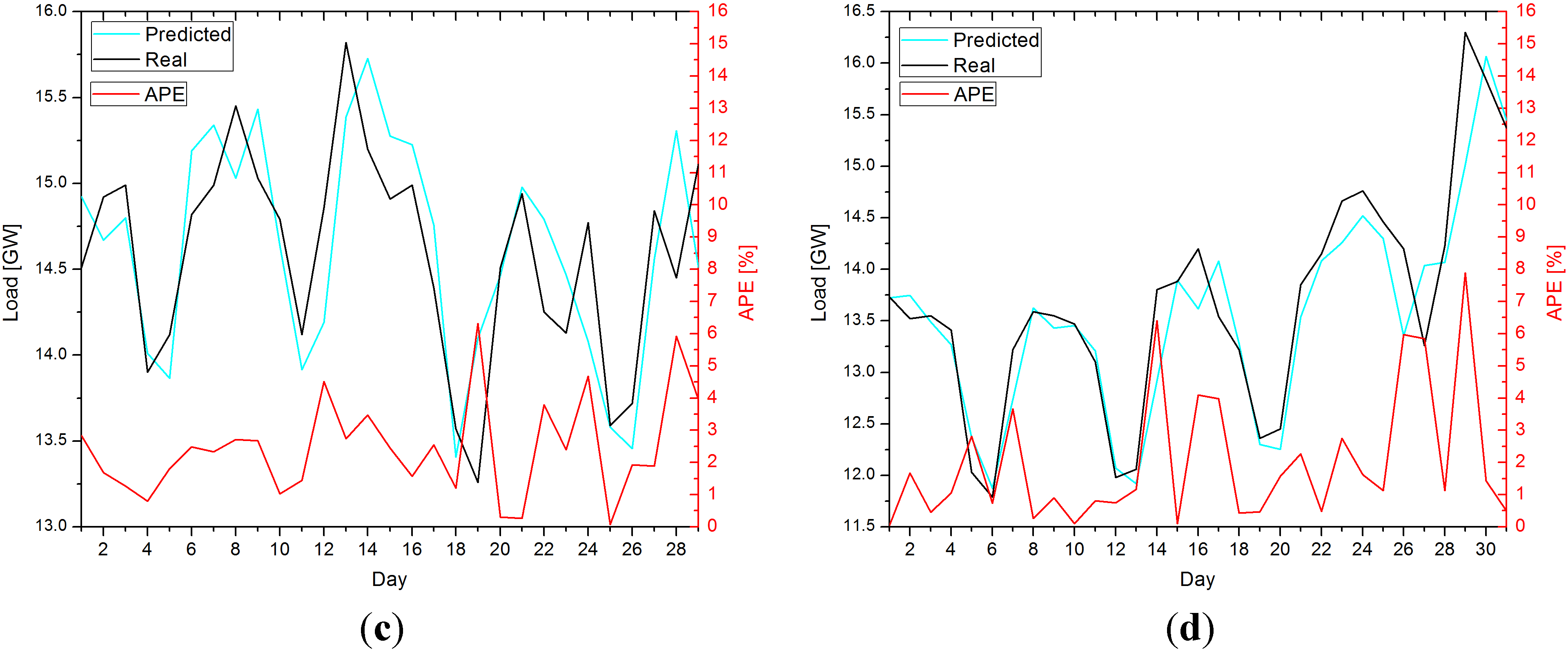
| Set | APE | ||
|---|---|---|---|
| Minimum | Average | Maximum | |
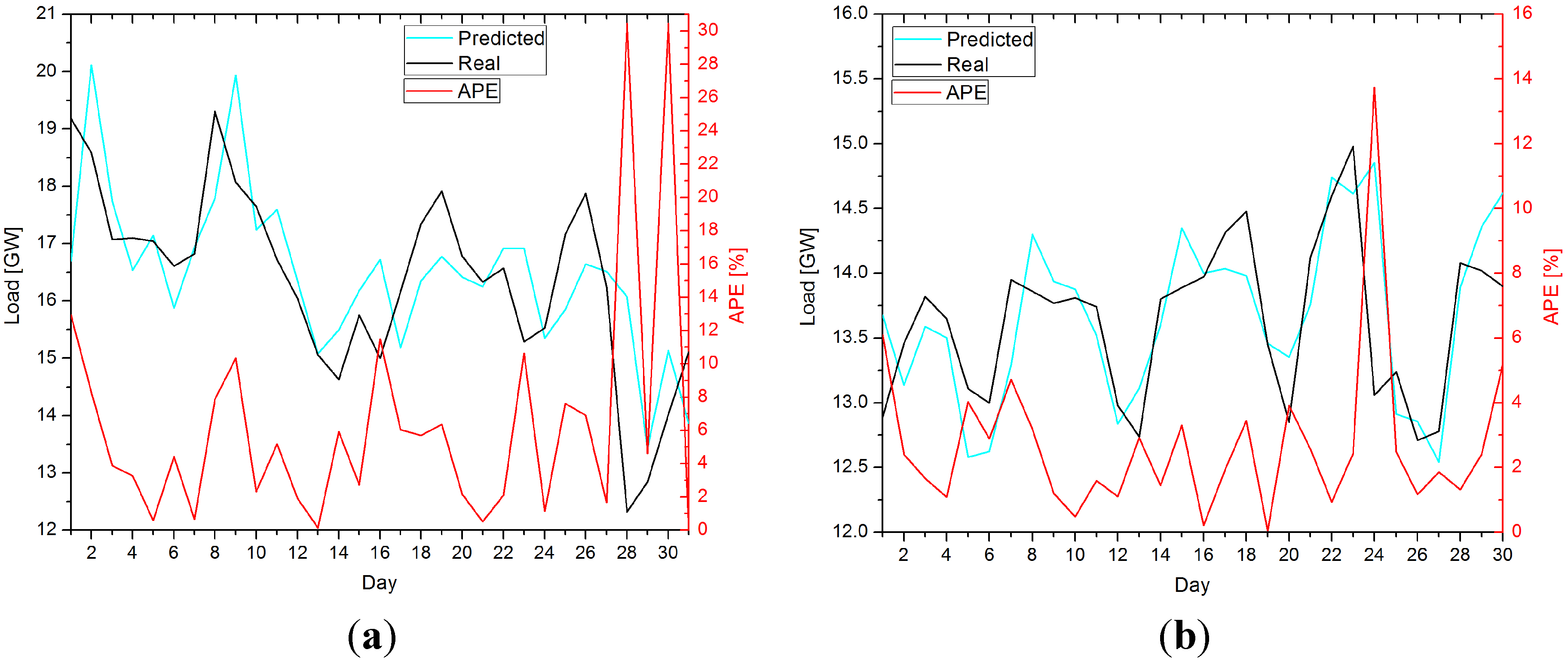
| August | 0.14 | 6.12 | 30.47 |
| November | 0.06 | 2.72 | 13.73 |
| February | 0.08 | 2.52 | 6.32 |
| May | 0.05 | 2.02 | 7.88 |
| Set | Input | MAPE | ME | ||||
|---|---|---|---|---|---|---|---|
| Minimum | Average | Maximum | Minimum | Average | Maximum | ||
| February | I2.5 | 2.43 | 2.92 | 4.38 | 0.58 | 0.96 | 2.05 |
| I5 | 4.48 | 5.33 | 7.04 | 0.92 | 1.55 | 2.14 | |
| I7.5 | 6.57 | 7.43 | 8.58 | 1.49 | 2.1 | 2.91 | |
| May | I2.5 | 2.26 | 3.16 | 5.71 | 0.63 | 0.98 | 1.6 |
| I5 | 4.14 | 5.12 | 6.14 | 0.88 | 1.44 | 2.26 | |
| I7.5 | 5.81 | 7.32 | 9.77 | 1.18 | 1.99 | 2.81 | |
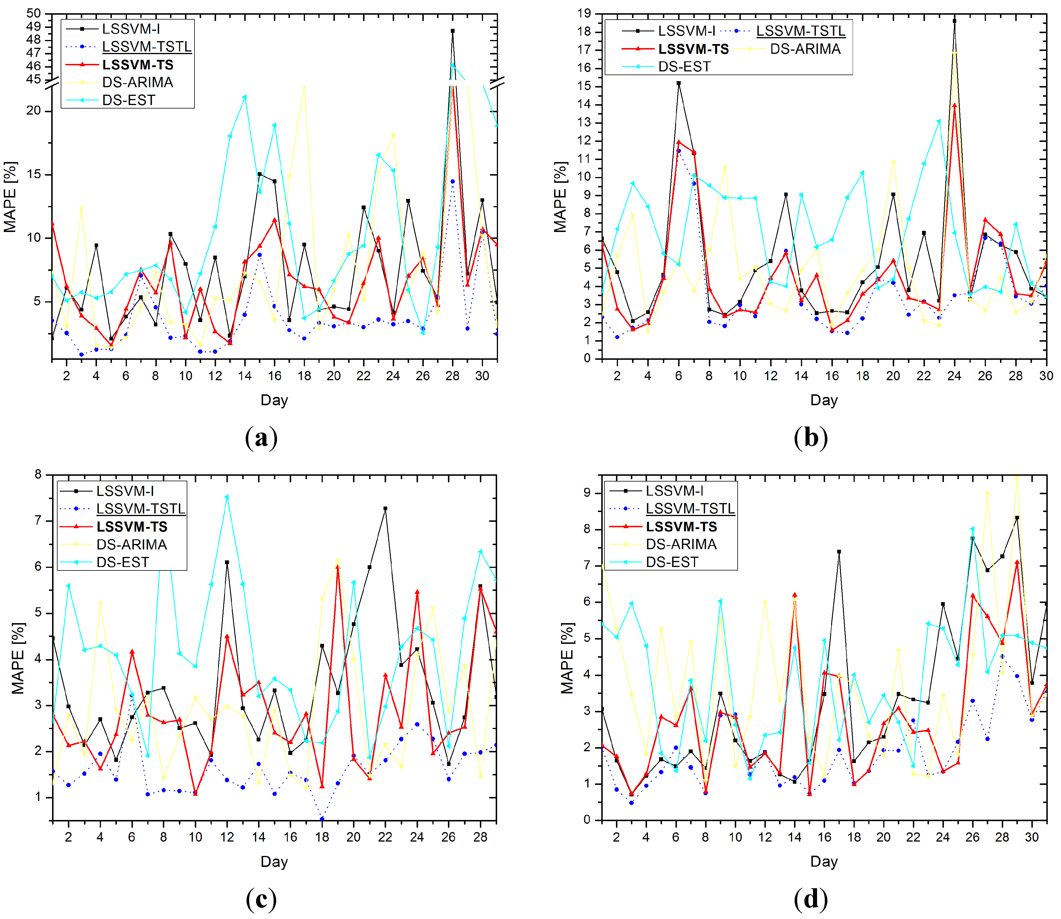
| Set | Model | MAPE (%) | ME (GW) | ||||
|---|---|---|---|---|---|---|---|
| Min. | Avr. | Max. | Min. | Avr. | Max. | ||
| August | LSSVM-I | 2.1 | 8.31 | 48.73 | 0.7 | 2.74 | 10.92 |
| LSSVM-TSTL | 0.85 | 3.73 | 17.47 | 0.4 | 1.29 | 3.95 | |
| LSSVM-TS | 1.55 | 7.09 | 32.06 | 0.63 | 2.29 | 7.99 | |
| DS-ARIMA | 1.38 | 8.44 | 30.1 | 0.59 | 2.17 | 6.6 | |
| DS-EST | 2.55 | 12.22 | 46.14 | 1.06 | 3.22 | 10.23 | |
| November | LSSVM-I | 2.09 | 5.56 | 18.62 | 0.62 | 1.64 | 5.41 |
| LSSVM-TSTL | 1.2 | 3.67 | 11.46 | 0.45 | 1.17 | 3.42 | |
| LSSVM-TS | 1.59 | 4.69 | 13.96 | 0.44 | 1.5 | 4.25 | |
| DS-ARIMA | 1.5 | 4.94 | 16.83 | 0.51 | 1.34 | 4.52 | |
| DS-EST | 3.42 | 6.95 | 13.11 | 1.06 | 1.81 | 2.69 | |
| February | LSSVM-I | 1.73 | 3.42 | 7.28 | 0.51 | 0.98 | 2.11 |
| LSSVM-TSTL | 0.53 | 1.63 | 3.22 | 0.23 | 0.64 | 1.63 | |
| LSSVM-TS | 1.07 | 2.9 | 6 | 0.39 | 0.94 | 1.97 | |
| DS-ARIMA | 1.22 | 2.97 | 6.15 | 0.39 | 1 | 2.01 | |
| DS-EST | 1.87 | 4.16 | 7.53 | 0.59 | 1.31 | 2.32 | |
| May | LSSVM-I | 0.71 | 3.35 | 8.33 | 0.26 | 1.01 | 2.93 |
| LSSVM-TSTL | 0.48 | 1.89 | 4.51 | 0.24 | 0.67 | 1.83 | |
| LSSVM-TS | 0.71 | 2.82 | 7.1 | 0.21 | 0.85 | 2.24 | |
| DS-ARIMA | 1.22 | 3.71 | 9.44 | 0.12 | 0.96 | 1.74 | |
| DS-EST | 1.15 | 3.86 | 8.02 | 0.47 | 1.21 | 2.63 | |
5. Conclusions
Acknowledgments
References
- Soliman, S.A.; Alkandari, A.M. Electrical Load Forecasting: Modeling and Model Construction; Butterworth-Heinemann: Burlington, MA, USA, 2010. [Google Scholar]
- Papalexopoulos, A.D.; Hesterberg, T.C. A regression-based approach to short-term system load forecasting. IEEE Trans. Power Syst. 1990, 5, 1535–1547. [Google Scholar]
- Christiaanse, W.R. Short-term load forecasting using general exponential smoothing. IEEE Trans. Power Appar. Syst. 1971, PAS-90, 900–911. [Google Scholar]
- Vähäkyla, P.; Hakonen, E.; Léman, P. Short-term forecasting of grid load using Box-Jenkins techniques. Int. J. Electr. Power Energy Syst. 1980, 2, 29–34. [Google Scholar]
- Irisarri, G.D.; Widergren, S.E.; Yehsakul, P.D. On-line load forecasting for energy control center application. IEEE Power Eng. Rev. 1982, PAS-101, 71–78. [Google Scholar]
- Mori, H.; Kobayashi, H. Optimal fuzzy inference for short-term load forecasting. IEEE Trans. Power Syst. 1996, 11, 390–396. [Google Scholar]
- Ranaweera, D.K.; Hubele, N.F.; Karady, G.G. Fuzzy logic for short term load forecasting. Int. J. Electr. Power Energy Syst. 1996, 18, 215–222. [Google Scholar]
- Rahman, S.; Bhatnagar, R. An expert system based algorithm for short term load forecast. IEEE Trans. Power Syst. 1988, 3, 392–399. [Google Scholar]
- Dillon, T.S.; Sestito, S.; Leung, S. Short term load forecasting using an adaptive neural network. Int. J. Electr. Power Energy Syst. 1991, 13, 186–192. [Google Scholar]
- Hippert, H.S.; Pedreira, C.E.; Souza, R.C. Neural networks for short-term load forecasting: A review and evaluation. IEEE Trans. Power Syst. 2001, 16, 44–55. [Google Scholar]
- Chen, B.-J.; Chang, M.-W.; Lin, C.-J. Load forecasting using support vector Machines: A study on EUNITE competition 2001. IEEE Trans. Power Syst. 2004, 19, 1821–1830. [Google Scholar]
- Hong, W.-C. Electric load forecasting by support vector model. Appl. Math. Model. 2009, 33, 2444–2454. [Google Scholar]
- Fan, S.; Chen, L. Short-term load forecasting based on an adaptive hybrid method. IEEE Trans. Power Syst. 2006, 21, 392–401. [Google Scholar]
- Amjady, N.; Keynia, F. Short-term load forecasting of power systems by combination of wavelet transform and neuro-evolutionary algorithm. Energy 2009, 34, 46–57. [Google Scholar]
- Wang, J.; Zhu, S.; Zhang, W.; Lu, H. Combined modeling for electric load forecasting with adaptive particle swarm optimization. Energy 2010, 35, 1671–1678. [Google Scholar]
- Hong, W.-C. Electric load forecasting by seasonal recurrent SVR (support vector regression) with chaotic artificial bee colony algorithm. Energy 2011, 36, 5568–5578. [Google Scholar]
- Borges, C.; Penya, Y.; Fernandez, I. Evaluating combined load forecasting in large power systems and smart grids. IEEE Trans. Ind. Inf. 2013. [Google Scholar] [CrossRef]
- Taylor, J.W. Short-term load forecasting with exponentially weighted methods. IEEE Trans. Power Syst. 2012, 27, 458–464. [Google Scholar]
- Mao, H.; Zeng, X.-J.; Leng, G.; Zhai, Y.-J.; Keane, J.A. Short-term and midterm load forecasting using a bilevel optimization model. IEEE Trans. Power Syst. 2009, 24, 1080–1090. [Google Scholar]
- Kebriaei, H.; Araabi, B.N.; Rahimi-Kian, A. Short-term load forecasting with a new nonsymmetric penalty function. IEEE Trans. Power Syst. 2011, 26, 1817–1825. [Google Scholar]
- Nose-Filho, K.; Lotufo, A.D.P.; Minussi, C.R. Short-term multinodal load forecasting using a modified general regression neural network. IEEE Trans. Power Deliv. 2011, 26, 2862–2869. [Google Scholar]
- Kandil, N.; Wamkeue, R.; Saad, M.; Georges, S. An efficient approach for short term load forecasting using artificial neural networks. Int. J. Electr. Power Energy Syst. 2006, 28, 525–530. [Google Scholar]
- Soares, L.J.; Medeiros, M.C. Modeling and forecasting short-term electricity load: A comparison of methods with an application to Brazilian data. Int. J. Forecast. 2008, 24, 630–644. [Google Scholar]
- Niu, D.; Wang, Y.; Wu, D.D. Power load forecasting using support vector machine and ant colony optimization. Expert Syst. Appl. 2010, 37, 2531–2539. [Google Scholar]
- Kelo, S.M.; Dudul, S.V. Short-term Maharashtra state electrical power load prediction with special emphasis on seasonal changes using a novel focused time lagged recurrent neural network based on time delay neural network model. Expert Syst. Appl. 2011, 38, 1554–1564. [Google Scholar]
- Cortes, C.; Vapnik, V. Support-vector networks. Mach. Learn 1995, 20, 273–297. [Google Scholar]
- Suykens, J.A.K.; Gestel, T.V.; Brabanter, J.D.; Moor, B.D.; Vandewalle, J. Least Squares Support Vector Machines; World Scientific Publishing Company: Singapore, 2002. [Google Scholar]
- ISO New England Historical Data. Available online: http://www.iso-ne.com/markets/hst_rpts/hstRpts.do?category=Hourly (accessed on 12 April 2013).
- Taylor, J.W.; de Menezes, L.M.; McSharry, P.E. A comparison of univariate methods for forecasting electricity demand up to a day ahead. Int. J. Forecast. 2006, 22, 1–16. [Google Scholar]
- Taylor, J.W. Short-term electricity demand forecasting using double seasonal exponential smoothing. J. Oper. Res. Soc. 2003, 54, 799–805. [Google Scholar]
© 2013 by the authors; licensee MDPI, Basel, Switzerland. This article is an open access article distributed under the terms and conditions of the Creative Commons Attribution license (http://creativecommons.org/licenses/by/3.0/).
Share and Cite
Božić, M.; Stojanović, M.; Stajić, Z.; Tasić, D. A New Two-Stage Approach to Short Term Electrical Load Forecasting. Energies 2013, 6, 2130-2148. https://doi.org/10.3390/en6042130
Božić M, Stojanović M, Stajić Z, Tasić D. A New Two-Stage Approach to Short Term Electrical Load Forecasting. Energies. 2013; 6(4):2130-2148. https://doi.org/10.3390/en6042130
Chicago/Turabian StyleBožić, Miloš, Miloš Stojanović, Zoran Stajić, and Dragan Tasić. 2013. "A New Two-Stage Approach to Short Term Electrical Load Forecasting" Energies 6, no. 4: 2130-2148. https://doi.org/10.3390/en6042130
APA StyleBožić, M., Stojanović, M., Stajić, Z., & Tasić, D. (2013). A New Two-Stage Approach to Short Term Electrical Load Forecasting. Energies, 6(4), 2130-2148. https://doi.org/10.3390/en6042130