1. Introduction
Gas turbine engines are highly complex systems consisting of static and rotating components, along with associated subsystems, controls, and accessories. They are required to provide reliable power generation over thousands of flight cycles while being subjected to a broad range of operating loads and conditions, including extreme temperature environments [
1]. Performance and reliability of aircraft turbofan engines gradually deteriorate over their service life due to degradation of the gas path components such as fan, compressor, combustor, and turbines [
2]. Common causes of degradation of the gas path components include compressor fouling, increase of the blade-tip clearance in the turbine, labyrinth seal leakage, wear and erosion, and corrosion in the hot sections. Foreign-object damage, caused by impingement of such foreign objects as birds, pieces of ice, and runway debris, will rapidly affect the component performance [
3,
4]. These physical faults lead to degradation of the health parameters, such as thermodynamic efficiency and flow capacity of individual gas-path components. Performance degradation, in turn, causes changes in the observable parameters, such as temperature, pressure, rotational speed, and fuel flow rate. Gas path health monitoring plays a critical role in improving safety, reliability, availability, and affordability. The cost-saving potential of such health evaluations is substantial, but only if the performance estimation are reliable [
5,
6].
Several approaches have been introduced to estimate the performance of gas turbine engines. Luppold proposed using a Kalman filter to estimate in-flight engine performance variations [
7]. Doel presented an assessment of weighted-least-squares-based gas path analyses [
8]. Depold applied expert systems and neural networks to gas turbine prognostics and diagnostics [
9]. Joly discussed gas-turbine diagnostics using artificial neural-networks for a high bypass ratio military turbofan engine [
10]. Kobayashi proposed a hybrid neural network-genetic algorithm technique for aircraft engine performance diagnostics [
11]. Ogaji reported a fuzzy logic approach for gas turbine fault diagnostics [
12]. Volponi compared the use of Kalman filter and neural network methodologies in gas turbine performance diagnostics [
13]. Dimogianoppoulos discussed aircraft engine health estimation via stochastic modeling of flight data interrelations [
14]. Li reported a novel nonlinear weighted-least-squares method, combined with the fault-case concept and the GPA index for effective gas-turbine fault detection, isolation and quantification [
15,
16,
17].
Compared to the data-based approaches, such as the neural network and fuzzy logic, the Kalman filter approach utilizes all model information available, can deal with the fact faults may not be known, and offers better estimation accuracy. Therefore, the variants of the Kalman filter are widely used for gas path analysis of gas turbine engines. Brotherton presented an approach that fused a physical model called self tuning on-board real-time model (STORM) with an empirical neural net model to provide a unique hybrid model called enhanced STORM (eSTORM) for engine diagnostics based on the Kalman filter [
18]. Volponi developed eSTORM, and provided a means to automatically tune for the engine model to a particular configuration as the engine evolved over the course of its life, furthermore, aligned the model to the particular engine being monitored to insure accurate performance tracking, while not compromising real-time operation [
19]. Simon D. applied constrained Kalman filtering, along with constraint tuning on the basis of measurement residuals, to estimate engine health parameters [
20,
21]. Litt proposed a real-time Kalman filter approach for estimation of helicopter engine degradation due to compressor erosion [
22]. Simon D.L. developed a systematic sensor selection approach and an optimal tuner selection approach for on-board self-tuning engine models, respectively [
23,
24]. Kobayashi reported application of a constant gain extended Kalman filter for in-flight estimation of aircraft engine health parameters [
25], and a baseline system based on Kalman filter for aircraft engine on-line diagnostics [
26]. Borguet presented adaptive filters to track gradual deterioration and rapid deterioration [
27]. Naderi proposed a nonlinear multiple model fault detection and isolation scheme for health monitoring of jet engines [
28].
The piecewise-linear dynamic scheduled models, from the component-level model of gas turbine engine, are required for gas path health monitoring via linear a Kalman filter in the flight envelope, and linearization errors that decrease the accuracy of performance estimation are inevitable. The EKF method is often used for state estimation with the assumption of weak nonlinear Gaussian systems [
29] in the references above, and the performance depends on how often Jacobians are updated. In practice the turbofan engine is a complex system with strong nonlinear and non-Gaussian noise. Recently, a popular solution strategy, sequential Monte Carlo sampling based particle filters, has been successfully used for the nonlinear and non-Gaussian state estimation problems, since it does not necessitate simplification of nonlinearity or any assumption of specific distributions [
30,
31,
32,
33,
34]. Orchard presented the implementation of a particle-filtering-based framework for calculating the probability of blade cracking and the remaining useful life in a turbine engine [
35]. Li introduced the particle filter into the application of unmanned aerial vehicle (UAV) engine fault prediction [
36], and then Gerasimos studied and compared nonlinear Kalman filtering methods and particle filtering methods for estimating the state vector of UAVs through the fusion of sensor measurements [
37]. Gross compared the performance of three nonlinear estimators—the extended Kalman filter, the sigma-point Kalman filter, and the particle filter—for global positioning system/inertial navigation system (GPS/INS) sensor fusion for aircraft navigation systems approaches [
38]. The EKF algorithm is used as the proposal distribution for PF importance sampling to avoid the particle degeneration in [
39,
40,
41].
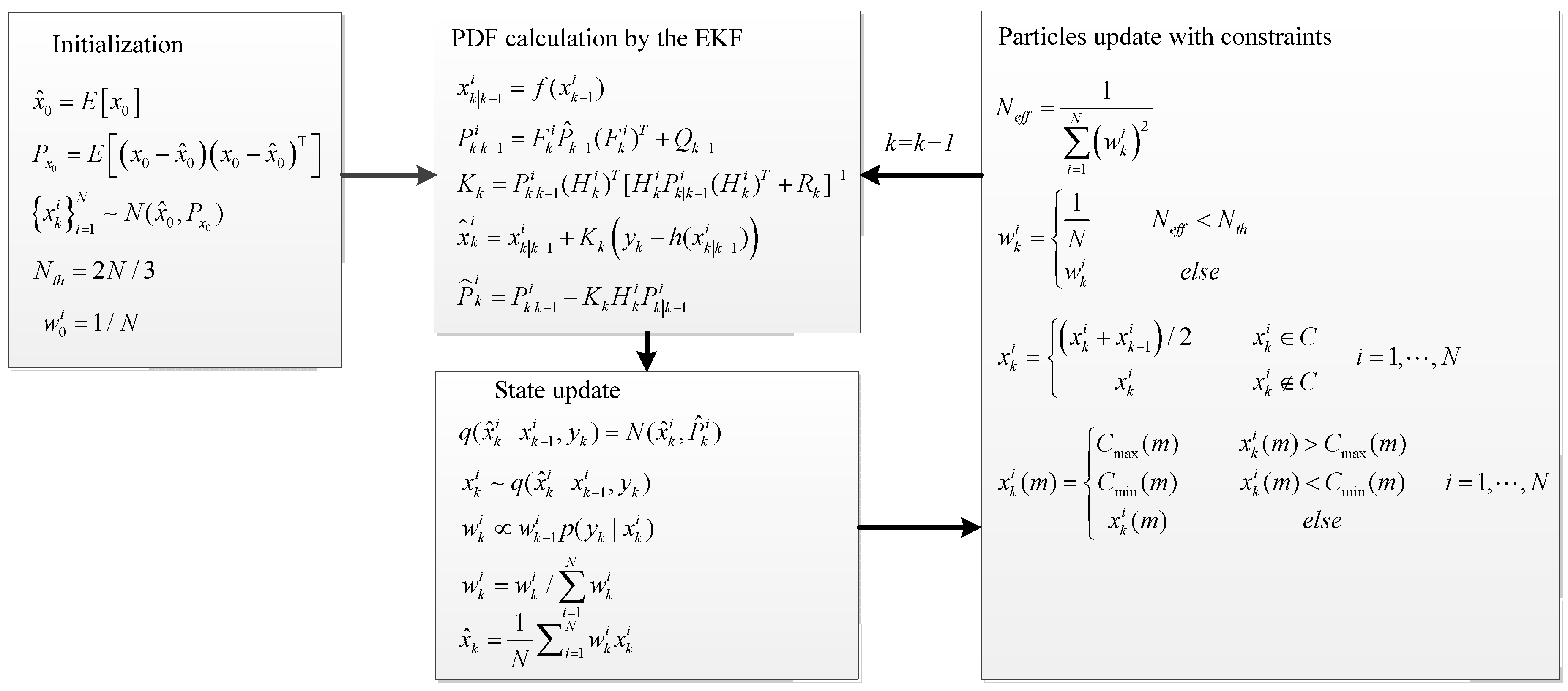
For the reasons described above, variants of the PF algorithm are used for the strong nonlinear and non-Gaussian systems. However, the PF has not been introduced to the problem of aircraft engine gas path performance estimation so far, which is usually strongly nonlinear and non-Gaussian. This paper presents the applications of turbofan engine gas path health monitoring based on particle filters, and gives a systematic comparison of the estimation accuracy and computational effort of various nonlinear filter based approaches to gas path performance estimation. Because the EKF requires a computational effort that is an order of magnitude lower than that of the UKF, the proposal distribution in the PF is calculated by the EKF in the paper. Considering the magnitude limitation of gas path degradation, the constrained extended Kalman filter particle filter is developed based upon the EKPF.
We emphasize that in this paper we are confining the problem to the turbofan engine health estimation in the presence of performance abrupt shifts and the gradual degradation with the cycle number. The performance estimation systems with Gaussian noise, non-Gaussian noise process noise are built up, and simulation results show that the constrained EKPF method enhances the robustness of PF algorithm against poor prior information. The comparisons of the EKPF and the cEKPF on estimate accuracy with the less measurement numbers are carried out, and validate that the estimate capability of the cEKPF outperforms that of the EKPF. The experiments and analysis show that compared to the known filtering approaches for aircraft engine gas path monitoring, the proposed cEKPF has better efficiency and is more compliant to the problem of health estimates with constraints.
This paper is organized as follows:
Section 2 discusses the formulation of different nonlinear filtering approaches containing the EKF, the PF, and the constrained EKPF.
Section 3 details the problem of turbofan health parameter estimation, along with the dynamic model that we use in our simulation experiments.
Section 4 shows some simulation results based on a nonlinear turbofan model. We see in this section the comparison of the nonlinear filtering approaches with the respect in the accuracy and the computational effort.
Section 5 presents some concluding remarks and suggestions for further work.
3. Turbofan Engine Gas Path Performance Estimation
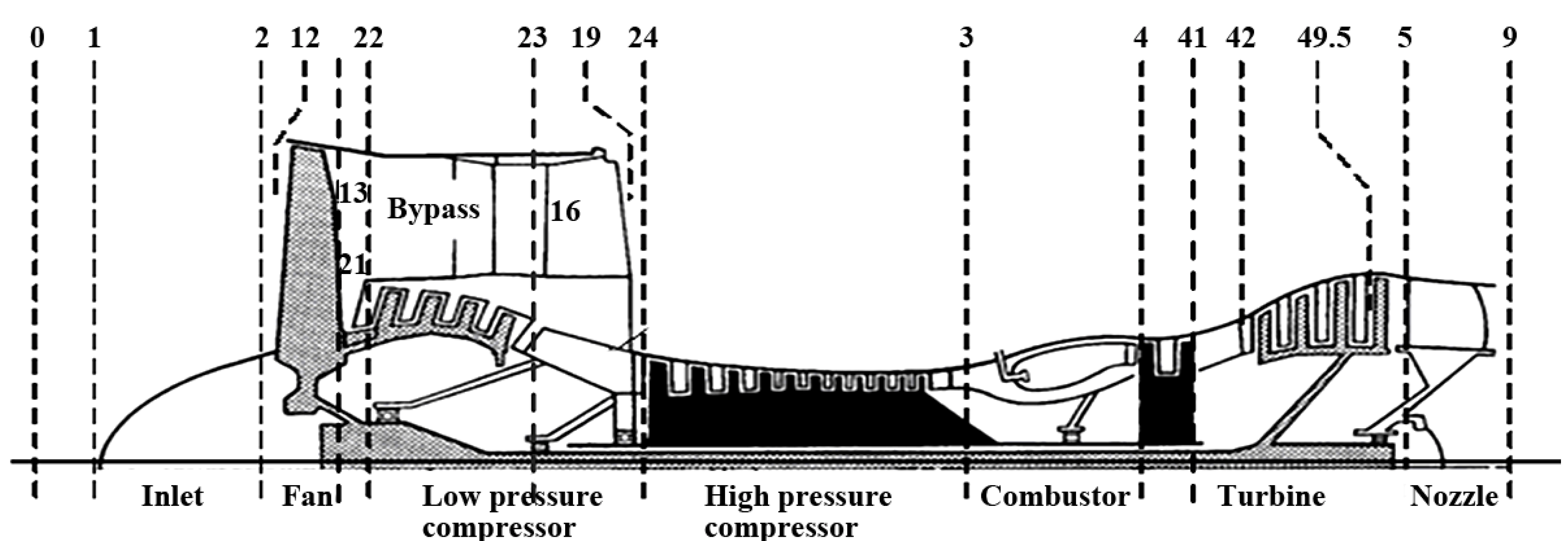
The engine is a high bypass ratio turbofan engine, see
Figure 2. A single inlet supplies airflow to the fan. Air leaving the fan separates into two streams: one stream passes through the engine core, and the other stream passes through the annular bypass duct and then leaves. The fan is driven by the low pressure turbine. The air passing through the engine core moves through the compressor, which is driven by the high pressure turbine. Fuel is injected in the combustor and burned to produce hot gas for driving the turbines. The air leaves the low pressure turbine (LPT) through the nozzle, which has a variable cross section area.
Figure 2.
Schematic representation of a turbofan engine.
Figure 2.
Schematic representation of a turbofan engine.
A turbofan engine mathematical model discussed in the paper consists of a number of individual components, each of which requires a number of input variables and generates one or more variables, denoted as Component Level Model (CLM). The model contains mathematical equations, maps, tables,
etc., which describe the thermodynamic relationships between various variables in the engine. In the CLM, we assume combustion delay is neglected; the component characteristics are unchanged with the Reynolds number, and zero-dimension flow. The thermodynamic parameters in cross sections of each component, such as the total temperature, total pressure, flow capacity, and efficiency, can be calculated as in references [
46,
47,
48]. The common operation of a turbofan engine in steady state follows flow capacity balance and power balance, and which are separated expressed as follows:
where
is the fan core duct outlet flow capacity,
the booster inlet one,
the booster outlet one,
the high pressure compressor (HPC) inlet one,
the combustor outlet one,
the high pressure turbine (HPT) outlet one,
the low pressure turbine (LPT) inlet one,
the LPT outlet one,
the nozzle core duct outlet one,
the fan bypass duct outlet one,
the bypass duct outlet one. Four cooling air streams
,
,
,
from the HPC are separately drawn in to cool the turbine inlet guide vane, blade-tip of the HPT and the LPT.
and
are the power produced by the HPT and LPT,
,
,
, and
are the power used for the HPC, accessories, fan, and booster,
and
are the high pressure spool efficiency and the low pressure spool efficiency, respectively.
The CLM in steady state has eight balance equations, seen in Equations (17) and (18), therefore, there are eight guess variables used to determine the engine steady operating condition, which are low pressure spool speed
, high pressure spool speed
, fan blade tip pressure ratio
, fan blade root pressure ratio
, booster pressure ratio
, compressor pressure ratio
, HPT pressure ratio
, and LPT pressure ratio
. The common operating expressions of the CLM in steady state can be denoted as the following nonlinear equations:
The common operating expressions of the turbofan engine in dynamics follows the flow capacity balance as same as the steady state ones in Equation (17). However, the two spools powers in dynamics are no longer balanced as in Equation (18), so they are replaced by the following equations defining the rotor dynamics:
where
, and
are the rotor inertias of the high pressure spool and low pressure spool. There are six guess variables,
, for the CLM in dynamics, and the current spool speeds are calculated via the speeds in the last step and the accelerations from Equation (20):
The nonlinear expressions both in steady state, Equation (19), and dynamics, Equation (21), are solved via Newton-Raphson approach. Iterative solution of nonlinear equations each step stops once one of the following conditions is satisfied: the maximum iteration number equals 10, or the iteration error is less than 0.01. The core rotating component efficiency/flow capacity is usually used to represent the aircraft engine gas path performance, seen in
Table 2, the degradations of which are denoted as health parameters as follows:
The health parameters and health parameter degradations are modeled in the CLM for the problem studied in the paper. The CLM is written using C language and packaged with dynamic link library (DLL) for use in the Matlab environment [
47,
49]. The outputs of function in DLL are the measurements, shown in
Table 3, and the inputs consist of height, Mach number,
,
, health parameters, and the noise. The CLM balances flow capacity (power) equations of the system is at a rate of 200 Hz, and the sampling frequency used for the nonlinear model health monitoring is 50 Hz. The discretized time invariant equations that model the turbofan engine from the dynamic CLM can be summarized as follows:
where
is the 2-element control vector,
the 2-element state vector,
the 7-element performance vector,
the 2-element environmental vector, and
the 9-element measurement vector [
29,
46]. The rapid degeneration and the gradual degeneration to the components are separately injected over time. Between measurement times their deviations can be approximated by the zero mean noise
, and
represents measurement noise. Nonlinear filtering approaches can be used with (23) to estimate the augment state vector
.
The controls, health parameters, and measurements are summarized in
Table 1,
Table 2 and
Table 3, along with their values at the design operating point considered in this paper, which is at sea level static conditions (
).
Table 3 also shows typical standard deviations for the measurements, based on experience, which are both used in the CLM and the estimators to build up the measurement noise covariance. Sensor dynamics are assumed to be high enough bandwidth that they can be ignored in the dynamic equations.
Table 1.
CLM turbofan model controls and nominal values.
Table 1.
CLM turbofan model controls and nominal values.
| Control | Acronyms | Nominal values |
|---|
| Fuel flow | | 2.5 kg/s |
| Variable nozzle aera | | 0.54 m2 |
Table 2.
CLM turbofan model health parameter, nominal value, standard deviation and degeneration maximum.
Table 2.
CLM turbofan model health parameter, nominal value, standard deviation and degeneration maximum.
| Augment state | Acronyms | Nominal value | Standard deviation | Deteriorate maximum (%) |
|---|
| Fan airflow capacity | | 1 | 0.0005 | −3.65 |
| Fan efficiency | | 1 | 0.0005 | −2.85 |
| HPC airflow capacity | | 1 | 0.0005 | −14.1 |
| HPC efficiency | | 1 | 0.0005 | −9.4 |
| HPT airflow capacity | | 1 | 0.0005 | 2.57 |
| HPT efficiency | | 1 | 0.0005 | −3.81 |
| LPT efficiency | | 1 | 0.0005 | −1.08 |
Table 3.
CLM turbofan model measurements, nominal values, and standard deviation.
Table 3.
CLM turbofan model measurements, nominal values, and standard deviation.
| Measurement | Acronyms | Nominal values | Standard deviation |
|---|
| Low pressure spool speed | | 3771 RPM | 0.0015 |
| High pressure spool speed | | 10241 RPM | 0.0015 |
| Fan exit pressure | | 172253 Pa | 0.0015 |
| HPC inlet temperature | | 707 K | 0.002 |
| HPC inlet pressure | | 344505 Pa | 0.0015 |
| HPC exit temperature | | 1078 K | 0.002 |
| HPC exit pressure | | 2940997 Pa | 0.0015 |
| LPT exit temperature | | 1086 K | 0.002 |
| LPT exit pressure | | 159367 Pa | 0.0015 |
4. Simulations and Analysis
In this section, the nonlinear filtering approaches discussed in this paper, and used for gas path performance estimation, are validated using Matlab. The normal operating parameters of the turbofan engine are depicted in
Table 1 and
Table 3. Gaussian noise whose magnitude is specified in
Table 3 is added to the clean simulated measurements to make them representative of real data. Two types process noise with the same covariance in
Table 2, Gaussian distribution and Rayleigh distribution, are separately introduced to build up the Gaussian system and the non-Gaussian one. The PDF of Rayleigh distribution is as follows:
The mean and covariance of Rayleigh distribution are separately , and this type process noise introduced into the system is a non-zero mean. In order to avoid health parameter degeneration estimates influenced by the non-zero mean process noise, the PDF of Rayleigh distribution is moved left with .
The engine’s health parameters are initialized to the values shown in
Table 2. Considering foreign-object damage to the engine, rapid degradations are carried out. The following rapid faults are simulated at 1 second: (1) −9% on SE2, (2) −3% on SE1, −9% on SE2, and 3% on SW3, which are labeled fault 1 and fault 2, respectively. Engine wear due to normal operation, gradual degeneration, is also simulated by linearly drifting values of nearly all health parameters, starting from 1 and with the maximum degradation in
Table 2 at the end of the sequence. Both in the PF and the constrained EKPF (cEKPF) framework, the number of particles is 50. The constraint value of each health parameter is set to more than 10% of its deteriorate maximum.
4.1. Rapid Deterioration Simulations
Rapid faults simulations with the three algorithms namely the EKF tool, the PF tool, and the cEKPF tool—are presented and discussed.
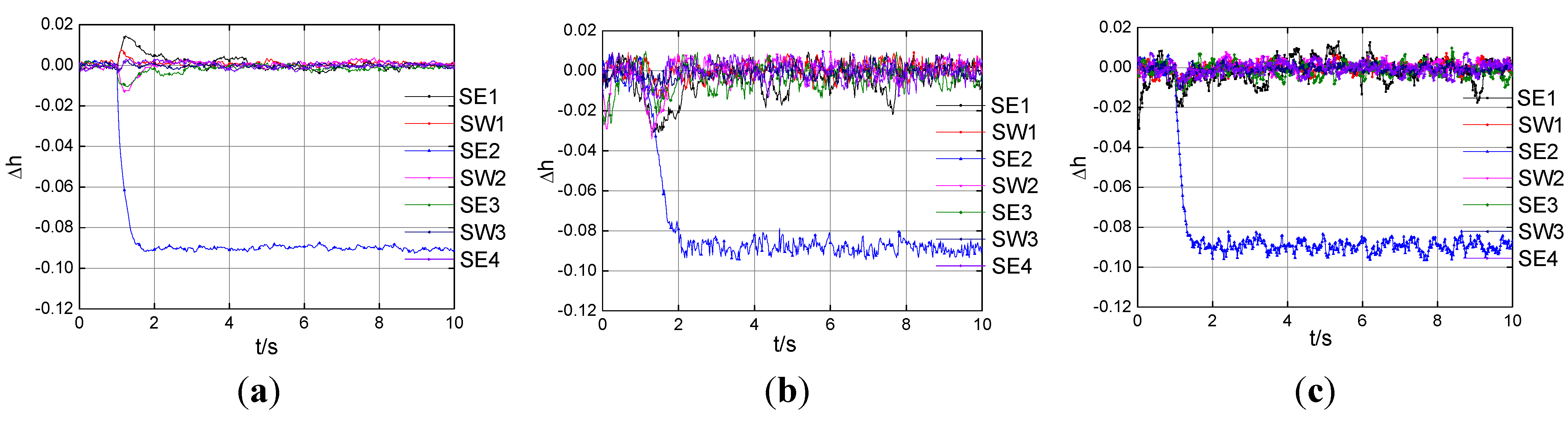
Figure 3 depicts the health parameters estimation, in the case of −9% on SE2 at 1s, with the three tools in the Gaussian system. As can be seen from
Figure 4, three health parameters separately track the performance shifts well in the Gaussian system under the Fault 2 conditions.
Figure 3.
Health parameters estimation with Gaussian noise under the Fault 1. (a) The EKF; (b) the PF; (c) the cEKPF.
Figure 3.
Health parameters estimation with Gaussian noise under the Fault 1. (a) The EKF; (b) the PF; (c) the cEKPF.
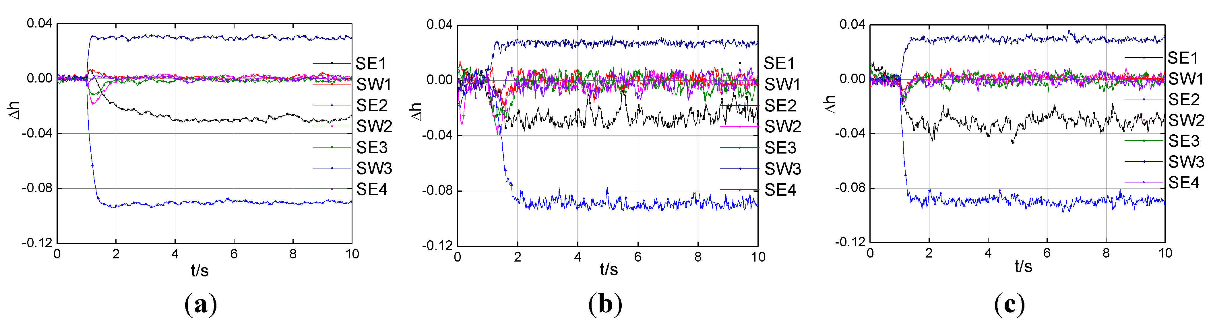
Figure 4.
Health parameters estimation with Gaussian noise under the Fault 2. (a) the EKF; (b) the PF; (c) the cEKPF.
Figure 4.
Health parameters estimation with Gaussian noise under the Fault 2. (a) the EKF; (b) the PF; (c) the cEKPF.
In order to compare the EKF, the PF, and the cEKPF more rationally, the process noise covariance matrices
Q and measurement noise covariance matrices
R are the same in three algorithms, respectively. The quality of the estimation performed by the three tools is assessed in terms of the estimation mean error (
) and its standard deviation (
) over the last 2 s of the sequence (100 samples):
where
is the true magnitude of deterioration of the
mth element of the health parameters, and
.
Table 4 reports the figure of merit defined by Equation (25) for the different fault-case with Gaussian noise that have been considered in the present study. For the rapid deterioration of Fault 1 and Fault 2, both the EKF and cEKPF perform a better accurate tracking of the engine conditions than the PF, which is confirmed by their estimation mean errors in
Table 4. The health parameters estimated with the PF jump seriously in
Figure 3(b) and
Figure 4(b), and its standard deviations are almost the biggest one compared to other two tools, as seen from the
Table 4. Bold numerical values correspond to the statistical characteristics of the degraded health parameters.
Table 4.
Mean error and standard deviation of the estimation with Gaussian noise.
Table 4.
Mean error and standard deviation of the estimation with Gaussian noise.
| | | Fault 1 | Fault 2 |
|---|
| | | EKF | PF | cEKPF | EKF | PF | cEKPF |
|---|
| (10−4) | SE1 | −4.42 | 52.53 | 0.55 | 2.89 | 3.03 | −2.88 |
| SW1 | 8.47 | 7.52 | 0.75 | 8.12 | 16.38 | 8.97 |
| SE2 | 0.08 | −3.29 | 4.27 | −1.28 | −1.95 | 1.81 |
| SW2 | 7.74 | 5.54 | 4.79 | 8.20 | 12.25 | 11.49 |
| SE3 | −11.22 | −34.73 | −14.07 | −8.56 | 7.71 | −8.23 |
| SW3 | −2.17 | −4.04 | −5.28 | −2.51 | −5.27 | −5.26 |
| SE4 | −3.08 | 17.28 | −4.49 | −3.02 | −24.76 | −4.98 |
| (10−3) | SE1 | 1.65 | 9.54 | 5.52 | 1.46 | 12.63 | 4.69 |
| SW1 | 0.89 | 4.39 | 2.41 | 1.27 | 4.36 | 2.18 |
| SE2 | 0.96 | 4.41 | 2.86 | 0.88 | 5.54 | 2.70 |
| SW2 | 1.05 | 4.19 | 2.04 | 1.03 | 5.24 | 2.39 |
| SE3 | 0.96 | 6.28 | 3.07 | 1.13 | 7.25 | 3.25 |
| SW3 | 0.81 | 2.60 | 1.55 | 0.97 | 3.26 | 1.61 |
| SE4 | 1.11 | 5.01 | 2.96 | 1.14 | 5.31 | 2.91 |
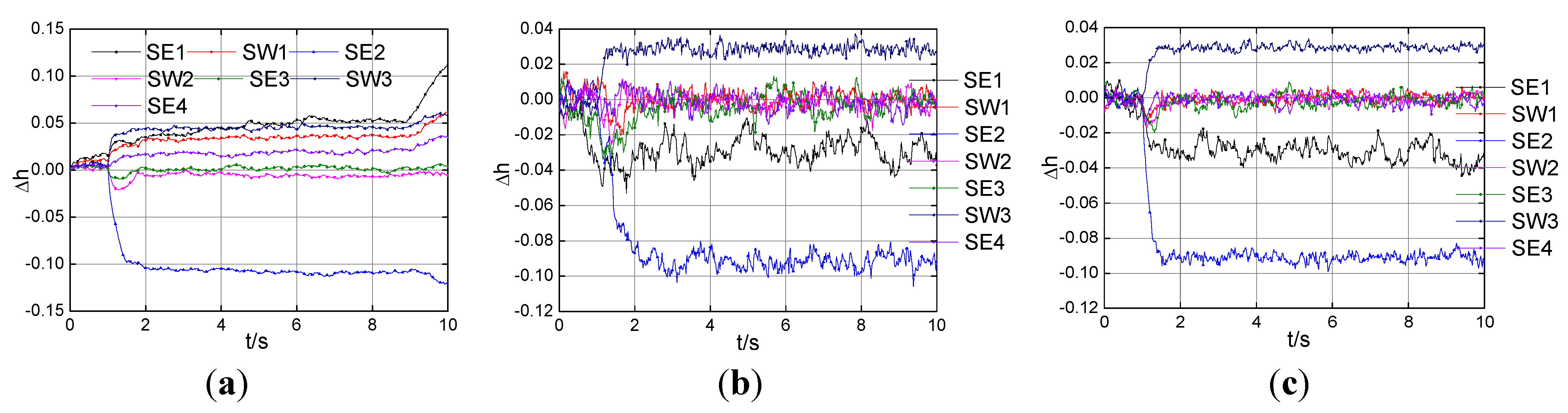
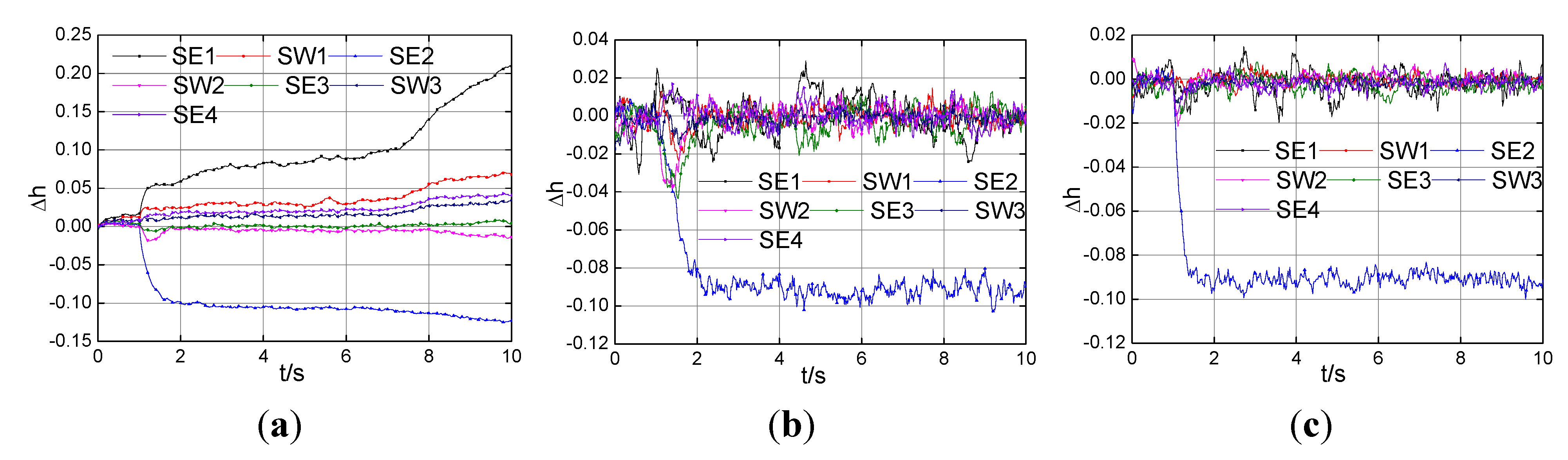
Figure 5 show the health parameters estimation, in the case of −9% on SE2 at 1 s, with the three tools in the nonlinear Gaussian system. We can see from the
Figure 5(a) that the health parameters SE1 and SE2 shift to 5% and −10% at nearly 2 s and then drift away, while the remaining health parameter delta values drift from zero. The estimated health parameter SE2 delta is about −9%, and the others about the zero, as shown in
Figure 5(b) and
Figure 5(c). Therefore, both the PF and the cEKPF can represent the engine conditions well, while the EKF produces misdiagnostics in the non-Gaussian system under the Fault 1 conditions. In
Figure 6, the three degraded health parameters are tracked well both with the PF and the cEKPF, except the EKF.
Figure 5.
Health parameters estimation with non-Gaussian process noise under the Fault 1. (a) The EKF; (b) the PF; (c) the cEKPF.
Figure 5.
Health parameters estimation with non-Gaussian process noise under the Fault 1. (a) The EKF; (b) the PF; (c) the cEKPF.
Figure 6.
Health parameters estimation with non-Gaussian process noise under the Fault 2. (a) The EKF; (b) the PF; (c) the cEKPF.
Figure 6.
Health parameters estimation with non-Gaussian process noise under the Fault 2. (a) The EKF; (b) the PF; (c) the cEKPF.
Table 5 presents mean error and standard deviation of the estimation defined by Equation (25) for the Fault 1 and the Fault 2 in the non-Gaussian system. For the rapid deterioration of the two fault modes with the non-Gaussian process noise, the cEKPF performs the most accurate estimation, then the PF, while the EKF fails in the estimation. It is confirmed by their estimation mean errors and standard deviations, especially the degraded health parameters that are indicated in bold in
Table 5.
Table 5.
Mean error and standard deviation of the estimation with non-Gaussian noise.
Table 5.
Mean error and standard deviation of the estimation with non-Gaussian noise.
| | | Fault 1 | Fault 2 |
|---|
| | | EKF | PF | cEKPF | EKF | PF | cEKPF |
|---|
| (10−3) | SE1 | 122.72 | 1.32 | −1.01 | 86.97 | 2.23 | −1.62 |
| SW1 | 43.90 | −0.11 | −0.43 | 37.75 | 0.44 | 0.11 |
| SE2 | −21.78 | −1.95 | −0.82 | −19.28 | −1.68 | −1.16 |
| SW2 | −6.84 | 0.04 | 0.07 | −5.57 | −1.66 | 0.03 |
| SE3 | 16.68 | −2.44 | −2.30 | 2.34 | −2.10 | −1.16 |
| SW3 | 20.32 | −0.42 | −1.41 | 16.99 | −1.29 | −1.23 |
| SE4 | 28.04 | 0.45 | −1.46 | 20.85 | −1.91 | −1.74 |
| (10−2) | SE1 | 4.32 | 0.97 | 0.60 | 1.52 | 0.67 | 0.53 |
| SW1 | 1.50 | 0.45 | 0.20 | 0.63 | 0.39 | 0.24 |
| SE2 | 0.61 | 0.42 | 0.28 | 0.31 | 0.41 | 0.25 |
| SW2 | 0.30 | 0.44 | 0.24 | 0.17 | 0.39 | 0.22 |
| SE3 | 0.25 | 0.70 | 0.32 | 0.20 | 0.60 | 0.3 |
| SW3 | 0.71 | 0.28 | 0.16 | 0.43 | 0.28 | 0.15 |
| SE4 | 0.85 | 0.57 | 0.30 | 0.51 | 0.48 | 0.29 |
4.2. Gradual Degeneration Simulation
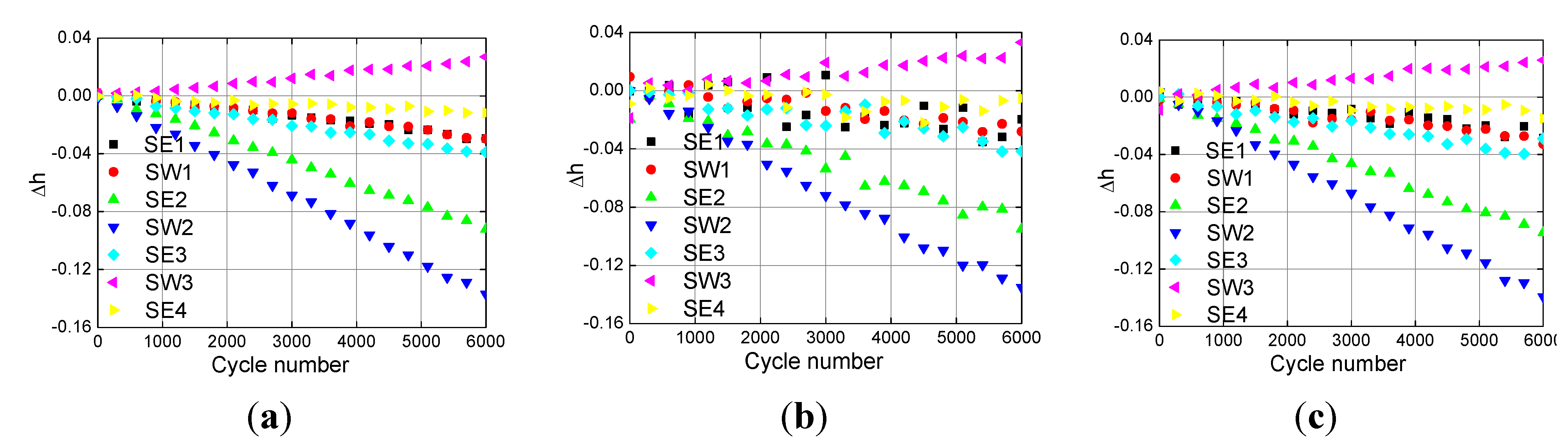
Gradual degeneration of a turbofan engine is simulated by linearly drifting values of nearly all health parameters, starting from their nominal values and with the following degradation at the end of the sequence (6,000 cycle number): −2.85% on SE1, −3.65% on SW1, −9.4% on SE2, −14.1% on SW2, −3.81% on SE3, 2.57% on SW3, −1.08% on SE4. There are 21 steady operating points in the whole degradation range.
Figure 7 and
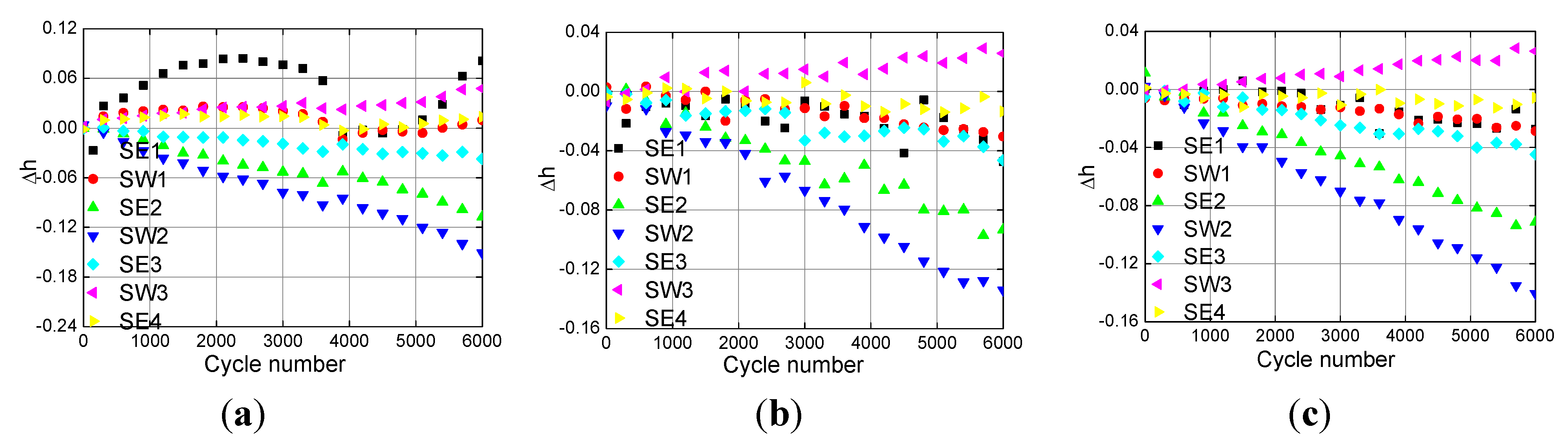
Figure 8 separately show the estimation performance of the three nonlinear filtering methods under the gradual degradation with Gaussian noise and non-Gaussian noise.
The health parameter degeneration value in the Gaussian system can be estimated with the EKF, the PF, and the cEKPF, while the PF performs less accurate tracking than the others, as shown in
Figure 7. When the Rayleigh distribution noise is introduced to the model, the estimation performance with the EKF is obviously decreased compared with
Figure 7(a) and
Figure 8(a).
Table 6 shows the estimation error square sum of 21 steady operating points in the whole degenerate range. In
Table 6 we can see that the performance of the PF and the cEKPF will not be much change with the various process noise.
Figure 7.
Health parameters estimation with Gaussian noise under the gradual degradation. (a) The EKF; (b) the PF; (c) the cEKPF.
Figure 7.
Health parameters estimation with Gaussian noise under the gradual degradation. (a) The EKF; (b) the PF; (c) the cEKPF.
Figure 8.
Health parameters estimation with non-Gaussian noise under the gradual degradation. (a) The EKF; (b) the PF; (c) the cEKPF.
Figure 8.
Health parameters estimation with non-Gaussian noise under the gradual degradation. (a) The EKF; (b) the PF; (c) the cEKPF.
Table 6.
Estimation error square sum at the steady state (10−2).
Table 6.
Estimation error square sum at the steady state (10−2).
| | EKF | PF | cEKPF |
|---|
| Gaussian system | 6.74 | 7.61 | 6.85 |
| Non-Gaussian system | 21.66 | 8.19 | 6.93 |
4.3. Computational Load
A computational load analysis was performed using simple Matlab profiling tools. Specifically, a unit-less computation load factor was determined by normalizing the Matlab m-file run time with the duration of operating data filtered. The computational time average of 20 tests is calculated, and the results are summarized in
Table 7.
Table 7.
Computational effort of the EKF, the PF, and the cEKPF.
Table 7.
Computational effort of the EKF, the PF, and the cEKPF.
| | System with Gaussian noise | System with non-Gaussian noise |
|---|
| | Fault 1 | Fault 2 | Fault 1 | Fault 2 |
|---|
| EKF | 7.7 | 7.7 | 7.8 | 8.3 |
| PF | 27 | 26.7 | 29 | 30.3 |
| cEKPF | 23 | 21.8 | 27.2 | 26 |
As indicated, the EKF requires a significantly less load than both the PF and cEKPF no matter whether Gaussian noise is injected into the system, although it performs poorly tracking the engine conditions in the non-Gaussian system. The PF and cEKPF load are heavily dependent on the number of particles used, however, the cEKPF consumes less time for estimation compared to the PF.
4.4. Potential Effect
The turbofan engine gas path health parameters are estimated by nonlinear filter approaches with all nine measurements in
Table 3 in the simulation above. While the number of available sensors for gas path analysis might decrease in practice,
i.e. one sensor failure. The following experiments that health parameters are estimated with eight measurements are carried out, and used to make comparisons of the EKPF and the cEKPF.
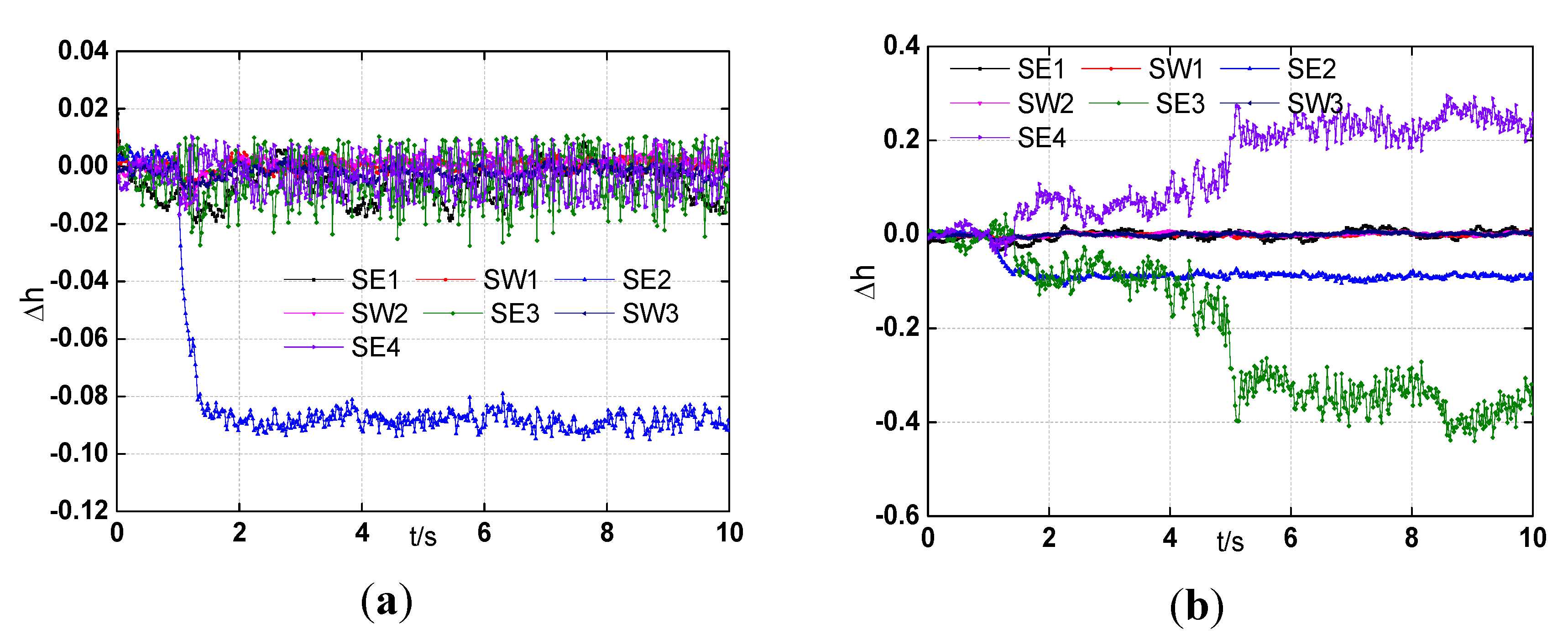
Figure 9 show that the health parameter estimates, in the case of Fault 1, with all measurements except the sensor
P5 in the Gaussian system by the EKPF and the cEKPF. As can be seen from
Figure 9(a), the estimate of
SE2 decreases to about −0.09 before 2s, and other health parameters are nearly unchanged, which are consistent with the Fault 1. However, in
Figure 9(b) there are three health parameter estimates,
SE2,
SE3, and
SE4, drifting from zero after 1s, false estimates are done via the EKPF.
Figure 9.
Health parameters estimation with all measurements except P5 in Gaussian system under the Fault 1. (a) The cEKPF; (b) the EKPF.
Figure 9.
Health parameters estimation with all measurements except P5 in Gaussian system under the Fault 1. (a) The cEKPF; (b) the EKPF.
Table 8 represents the mean error sum of the health parameter estimates,
, with all measurements except one sensor in turn in the Gaussian system. We can see that the health parameter estimations can’t be implemented via the EKPF under three conditions of sensor selection: all measurements except
nL, except
P13, or except
T24, respectively. Although the estimates are convergent and the
MSE can be calculated by the EKPF under the remaining six sensor selected condition, the
MSE are much bigger than that by the cEKPF. Therefore, compared to the EKPF, the cEKPF is an effective estimator and can be still used for gas path health monitoring with one less sensor.
Table 8.
Estimation error square sum with the eight measurements in Gaussian system.
Table 8.
Estimation error square sum with the eight measurements in Gaussian system.
| | nL | nH | P13 | T24 | P24 | T3 | P3 | T5 | P5 |
|---|
| EKPF | x | 0.875 | x | x | 1.001 | 0.632 | 0.284 | 1.552 | 0.909 |
| cEKPF | 0.276 | 0.207 | 0.188 | 0.195 | 0.193 | 0.187 | 0.191 | 0.198 | 0.196 |
The particle number is an important parameter in variants of the PF algorithm, and the estimate accuracy and computational load rest with the particle scale.
Table 9 shows the comparisons of estimate performance with nine measurements by the cEKPF under three particle scales:
N = 30,
N = 50, and
N = 100. We can make some interesting observations from the
Table 9, the
SME decrease and the computational load steadily increase as the particle number increases from 30 to 100 both under Fault 1 and Fault 2. Compared to the particle number increase from 30 to 50, there does not appear to be evidently any improvement in the estimation accuracy when the number goes from 50 to 100. The particle number equal to 50 is reasonable in this case for gas path health monitoring.
Table 9.
Comparisons of estimate performance by the cEKPF under different particle scales.
Table 9.
Comparisons of estimate performance by the cEKPF under different particle scales.
| | Fault 1 | Fault 2 |
|---|
| | N = 30 | N = 50 | N = 100 | N = 30 | N = 50 | N = 100 |
| SME(10−2) | 0.366 | 0.343 | 0.342 | 0.472 | 0.438 | 0.432 |
| Time(s) | 14.1 | 23 | 40.8 | 14.1 | 21.9 | 40.3 |
5. Conclusions and Future Work
Within this study, a widely used nonlinear estimation method, the particle filter based on Monte Carlo sampling algorithms, is implemented for gas path performance monitoring for turbofan engines. Because of particle degeneracy in the generic PF framework, the EKF is introduced to use the latest observation value to amend the state transition model of particles and its amount of calculation is not big. Considering the degradation magnitude of health parameters is within a certain range during the on-wing cycle, the constrained strategy of particle update is designed and combined with the EKPF, and then the detailed constrained EKPF is proposed and presented.
This paper has compared the three nonlinear filters based estimation approaches, the EKF, the PF, and the constrained EKPF, for the evaluation of turbofan engine gas path health. The health monitoring system with Gaussian noise and non-Gaussian noise (Rayleigh distribution process noise), keeping the same process noise variances, are set up separately. The accuracy and computational load under the different cases of abrupt faults and gradual degradation are used to evaluate the three filtering methods. Compared to the EKF, the PF and the cEKPF perform with more adaptability to the non-Gaussian system. According to the experiments on health parameter estimates with less measurements, we can see that the effect of cEKPF is obviously much better than that of the EKPF. The particle number influenced to the estimate accuracy and computational effort is discussed in the cEKPF, and the better particle scale for gas path health monitoring is selected. The improvements brought by the EKF with constrained mechanism to a generic PF have enhanced the computational effort of the PF algorithm.
In summary, the proposed cEKPF is an effective way to estimate health condition for complicated machines with undetermined noise. The non-Gaussian system is defined as the system with the Rayleigh distribution process noise in present paper, while the non-normal distribution process noise, the non-normal distribution measurement noise, or both of them introduced to the system will produce the non-Gaussian system. Therefore, it would be interesting to see how the conclusions of this paper might change with the other forms of non-Gaussian system.

