1. Introduction
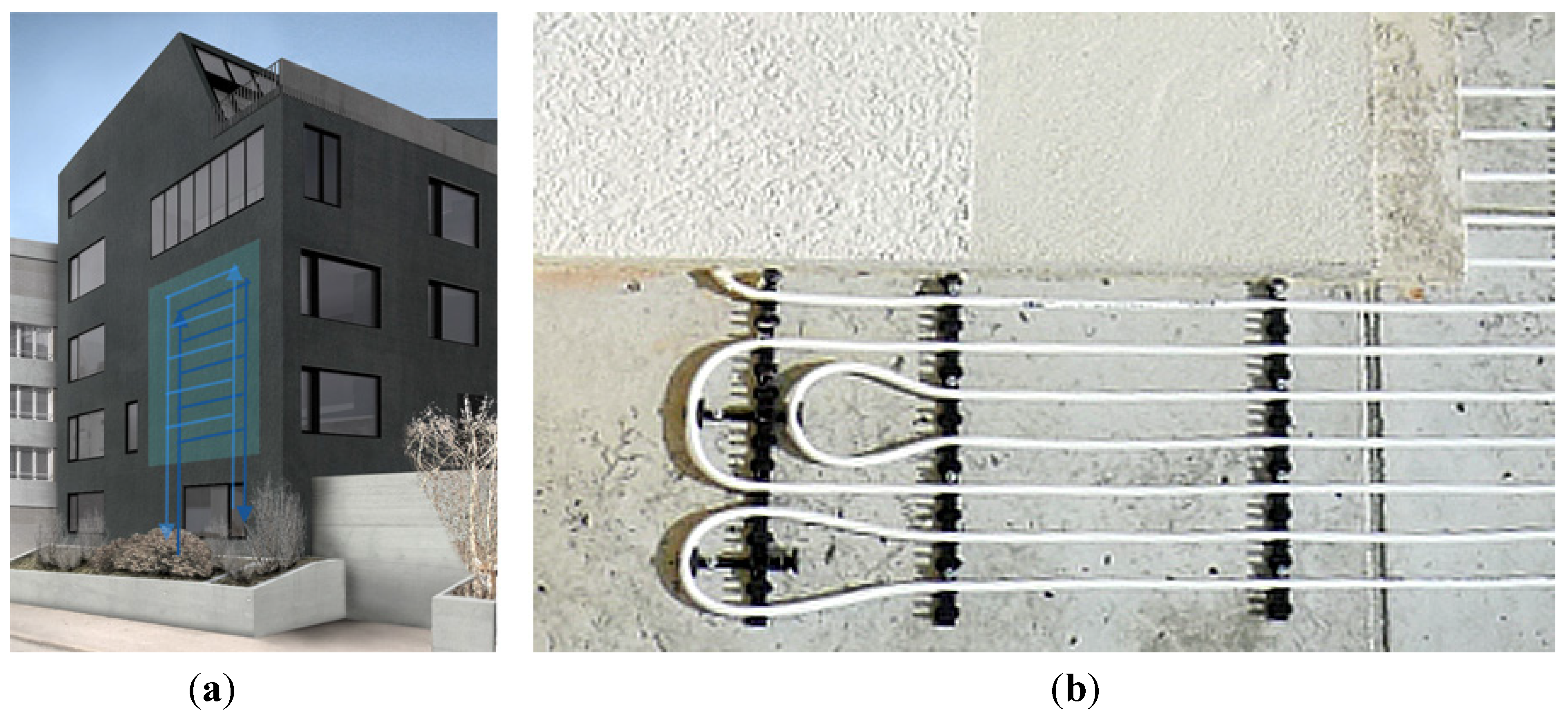
We have developed a building insulation concept that utilizes renewable geothermal energy to actively reduce the dispersion of exergy from the conditioned space to the environment. We have named it ALEGIS (for Active Low Exergy Geothermal Insulation System). The new concept improves building performance by using the temperature of the ground in a small layer of the building facade. Small pipes are embedded in a thin outer layer of the facade. The layer consists of the simple piping structure attached with thermally conductive cement and covered in a thin thermally resistive plaster. A geothermal heat exchanger and a small circulation pump provide fluid at ground temperature such that the wall has a constant temperature. This eliminates the effects of lower outside temperatures, reduces building heat loss, and it utilizes the heat of the ground directly. Still, a heat pump or heating system has to be used to provide the base heat demand. In this case the heat demand is reduced and at a constant level, which allows the heat pump to be optimized for nearly constant conditions. A rendering and a prototype installation is shown in
Figure 1.
Figure 1.
(a) Rendering of the ALEGIS system on a building with a horizontal distribution across a section of wall; (b) Prototype installation of piping under a layer of insulation plaster on a concrete wall.
Figure 1.
(a) Rendering of the ALEGIS system on a building with a horizontal distribution across a section of wall; (b) Prototype installation of piping under a layer of insulation plaster on a concrete wall.
During cold outside conditions the same reduction in heat transfer through the facade is achieved by ALEGIS as would be achieved by much thicker passive insulation. The combination of high performance with a thin installation makes the system ideal for renovation. Especially for renovations where a heat pump could provide the optimal performance, but the heat loss from the building is too high to be effectively provided by a heat pump. Also this provides a second function for the ground source heat exchanger, which can be expensive to install. It provides the facade with the ALEGIS heat barrier, as well as an ideal source for a heat pump.
1.1. Background
The impetus for this seemingly strange idea of supplying heat to the outside of a building came from the combination of research into low exergy systems [
1,
2,
3,
4,
5,
6], combined with a desire for high performance facades without excessive thickness. Based on the awareness of the disadvantages of very thick passive house walls [
7], along with the need for thin renovation options, the ALEGIS concept was developed. If one actively heats the outer side of the wall construction, a virtual translation of the wall into a warmer climate zone is achieved. The building feels as if it is an earth-sheltered structure, which have been shown to have great performance benefits [
8]. Not only that, but this active system has the ability to be turned off, which makes it adaptable to the potential problem that heavily insulated buildings have of overheating. This allows the system to selectively eliminate large thermal gradients from extreme cold while remaining adaptive to warmer conditions.
The higher temperatures attainable from ground source heat exchangers in winter compared to the environmental temperatures, provides a large potential. It improves the performance of heat pumps measured by their coefficient of performance (COP), which is the ratio of heat supplied to work input. With ALEGIS, we have gone one step further and found a way to utilize this higher temperature directly in the building structure to reduce heat demand.
The concept is possible because the ground temperature remains constant below a depth of around 5 m [
9]. The volume of earth creates an infinite heat sink or heat source limited only by the rate at which heat can be deposited or extracted [
10]. In areas of high geological activity, high temperature sources can be found beneath the surface, but in most temperate locations the temperature is between 8 and 16 °C, and usually increases about 2–3 degrees with each 100 m of depth [
9]. In layers closer to the surface, a strongly damped oscillation is observed due to the changing ambient outside conditions. Our analysis is based on these typical conditions and the winter design conditions of Zurich, Switzerland.
2. Methods
2.1. Wall Parameters and Dimensioning
For the analysis of the temperature distribution in an actively insulated wall, the following parameter values are assumed: The solid wall being a concrete construction has a thickness of 0.18 m and a thermal conductivity of 0.72 W/mK. The plaster used to hold the tubes for the active insulation system has the same thickness as the diameter of the tubes, i.e., 0.01 m, and it has a higher thermal conductivity of 1 W/mK to encourage uniform temperature distribution in the piping layer. Any insulation material used in the model is assumed to have a thermal conductivity of 0.04 W/mK, conservative for spray foam or insulation board. For analyses not dealing with insulation thickness, a default thickness of outer insulation that covers the piping of 2 cm is chosen. The working fluid has an average temperature of 10 °C and a 2 °C temperature drop is fixed across the wall system. By default a tube spacing of 5 cm is assumed which corresponds to 20 pipes passing within 1 m height of the wall. Room temperatures are fixed at 20 °C, and the outside design temperature is at −10 °C. For the calculation of the convective heat fluxes the convection coefficient for inside is assumed at 8 W/m2K and for outside is assumed at 25 W/m2K. Radiant losses, even at the higher wall temperature, would be negligible compared to convective losses. The potential gains due to solar irradiation are ignored for this analysis to maintain a neutral case for comparison.
2.2. Wall Temperature Distributions and Tube Spacing
The heat fluxes in the different layers of the wall construction must be evaluated in order to compare typical static insulation to this active concept. It is important to determine the interface temperature in the wall where extra heat from ALEGIS is supplied. This temperature depends on the small amounts of insulation installed above and below the piping system as well as the piping spacing. The temperature in this layer will vary between the piping, which will influence the performance of the system and will determine the necessary insulation and tube spacing for the system.
A simple model estimates the temperature profile in the piping layer of the wall. Assuming one-dimensional heat transfer though the wall and regular tube spacing, an average temperature was calculated for the piping layer based on the heat flux through the wall-area containing a tube and the wall-area between tubes given in Equation (1). For cold outside conditions the actual maximum temperature in the piping layer would be found at the pipe, and the minimum would be found at the midpoint between two pipes. Assuming that the vertical temperature gradient at these two points would be zero (two zero-slope constraints), a simple third-order polynomial was determined to approximate the profile and the minimum temperature between the pipes. The polynomial coefficients were found by setting the integral over the one wall section equal to the average temperature from Equation (1).
2.3. Comparison to Static Insulation
The active insulation system fixes the temperature under the insulation so that the outside temperature has minimal effect on the wall. We evaluate the amount of passive insulation required to achieve a temperature underneath it that is equivalent to the average temperature generated by the active insulation. This equivalent thickness depends on the outside temperature; the colder the outside temperature is, the more static insulation is required to match the performance of the active system. For the analysis we assumed an inside temperature of 20 °C and evaluated a range of outside conditions.
The equivalent static insulation is calculated by first determining the heat flux in the active system between the inside temperature and the average piping layer temperature. This heat flux is then used with the actual outside temperatures to calculate an equivalent thermal resistance,
Req, of the active system, Equation (2). This equivalent thermal resistance can then be used with a standard insulation material to determine the thickness required to achieve the same performance, Equation (3)
2.4. System Performance Comparison
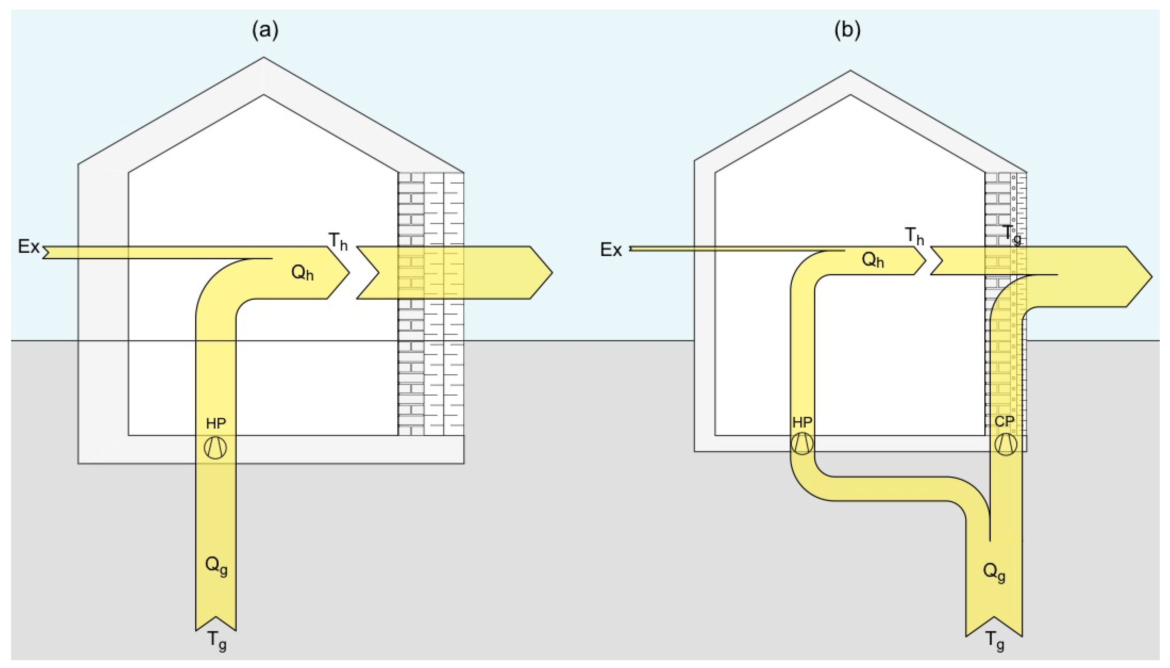
The flow of heat from the ground into the piping layer of the wall requires pumping energy. Instead of increasing the temperature of this heat using a heat pump so that the building can be directly heated, part of the ground heat is used directly in the wall to reduce the heat demand of the building. This allows a comparison of a typical heat pump COP, and the overall COP of this active system. The active system COP can be considered in two ways. First, a simple pump COP can be described as the amount of heat that is supplied to the wall directly relative to the pumping work input. Second, a virtual heating COP can be defined as the amount of heat loss that is avoided or blocked by the piping layer in the wall relative to the pumping work input to achieve this effect. The second ratio presents the most realistic comparison to the heat pump COP because it relates directly to the heat demand of the building. This comparison is illustrated in
Figure 2.
In order to make such a COP comparison the actual pumping costs must be estimated, and these depend on the building size and outside temperature. Therefore a very generic building model is employed along with weather data for Zurich, Switzerland [
19].
A cubic building was assumed with 10 m by 10 m walls and roof. It was assumed that the shell of the cubical building was constructed with 18 cm concrete wall construction as described above. This combined with a horizontal cross flow topology, pipe spacing, and pipe diameters allowed for a calculation of the pressure drop of the system. It also allowed an estimation of the necessary ground source heat exchanger size and depth. The pumping costs of the geothermal connection for each wall could then also be considered.
The total heating season heating demand of the building was evaluated for the cases (a) and (b) in
Figure 2. We calculated the exergy demand of the integrated heat pump system for case (a) and the heat pump and circulation pumps for case (b). This includes the analysis of the active wall performance with the ground source heat exchanger loading and its extra pumping requirement, as well as the pumping demand for the wall itself.
Figure 2.
Heat pump vs. circulation pump + heat pump. (a) Standard heat pump energy flow, heat is brought up from the ground, Qg, at ground temperature, Tg, and a heat pump, HP, uses exergy, Ex, to increase the temperature for heating to Th to meet the heat demand, Qh; (b) Ground heat is used by the heat pump, HP, as in (a), and also in circulation pump, CP, so that the wall temperature becomes equal to the ground temperature, Tg, and the building heat demand, Qh, is reduced by the active insulation.
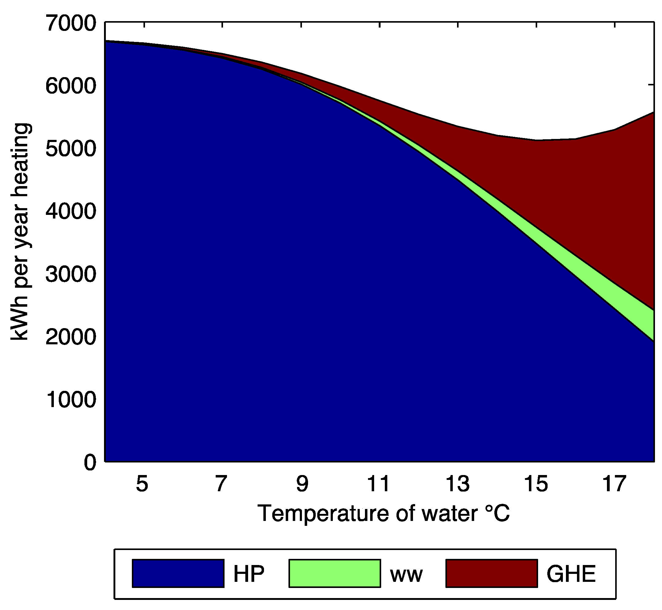
The annual temperatures during winter, taken from weather data for Zurich, Switzerland, produced an hourly heating demand for the sample 10 × 10 × 10 m building. The system performance was calculated using three scenarios for the building insulation. These were the active insulation system, the static insulation of equivalent thickness, and finally the un-insulated brick wall, which provided a basis for potential benefit in renovations to older constructions. The cooling case for summer was not considered for this case because the geothermal temperature acquired in Zurich can be used directly for cooling inside without a heat pump, making comparison to direct use in the wall irrelevant. Also, the active layer was turned off when the outside temperatures were high enough to eliminate the benefit of the ground temperature in the wall, and then the heat loss was calculated based on the passive performance of the active system.
2.5. Wall and Ground Heat Pressure Losses
The total system pressure loss of the active insulation system and the ground source loop must be evaluated in order to estimate the pumping costs. Variable speed pumping is assumed to control the mass flow in the system to maintain a temperature drop across the wall of 2 K. Therefore the pressure losses are also dependent on only the piping layer heat loss, and thus the outside temperature.
For the calculation of the pressure loss, both major and minor losses were considered. The major pressure loss in the wall is calculated based on the number of tubes, their diameter and their length for each wall section of the building using standard fluid dynamics methods [
20]. The minor losses occur in the fittings that connect the parallel branches to the major branches. For each horizontal branch a loss factor of 1 is assumed at each T-junction along with a factor of 0.08 and 0.13 for contraction and expansion respectively, and the large major branch losses are negligible.
For the ground heat exchanger loop, the performance was checked to confirm the assumed temperatures and flow rates coming into the active insulation system. This was not directly integrated into the model. The calculations are based on the work of Claesson and Eskilson in Sweden [
21] using the Earth Energy Storage (EED) software. The loadings for the 10 × 10 m surfaces of the cubic building were compared with EED to check for adequate U-tube borehole length and verify the assumed temperature input coming out of the ground heat exchanger system. From this a single 300 m deep U-tube heat exchanger is used for the analysis with 5 cm diameter connected to the active insulation system with the piping network on each 10 m × 10 m surface. The total efficiency of the circulation pumps were taken to be 25% in accordance with commercially available models. The exergy for a circulation pump is calculated based on the operating conditions expressed by the total pressure rise and the flow rate, and the total pump efficiency shown in Equation (4):
With the determined pump work, the equivalent COP of the system can be calculated. The heat demand reduction achieved can be used to create a ratio with the work input of the circulation pump. This was used in the comparison to heat pump performance in standard installations.
2.7. Low Exergy System Analysis
The low exergy aspect of the active low exergy geothermal insulation system comes from the process of its invention and the change in the flow of exergy through the wall by the system. The invention of the system comes from the idea of the flow of exergy into a heat pump, where the electricity input is the exergy input and usually the heat source comes from the reference environment and has no exergy. The idea that ground heat could then be considered as free exergy led to the idea of utilizing it in the wall to change the exergy flow out of the building. Basically, we made the reference environment of the building be the ground instead of the outside air. Meggers
et al. has expanded on the theoretical implications for these spatial (or temporal) shifts in reference environment [
25]. The change in the flow of exergy through the wall is actually shifted because the value of the room air temperature compared to the ground temperature is less than compared to the colder winter outside air. Instead of using the ground temperature to just decrease the temperature-lift of the heat pump and increase its COP, we use it to also decrease the temperature-fall of the building.
3. Results and Discussion
3.1. Wall Temperature Distributions
The resulting temperature distributions in the piping layer are shown in
Figure 3 and
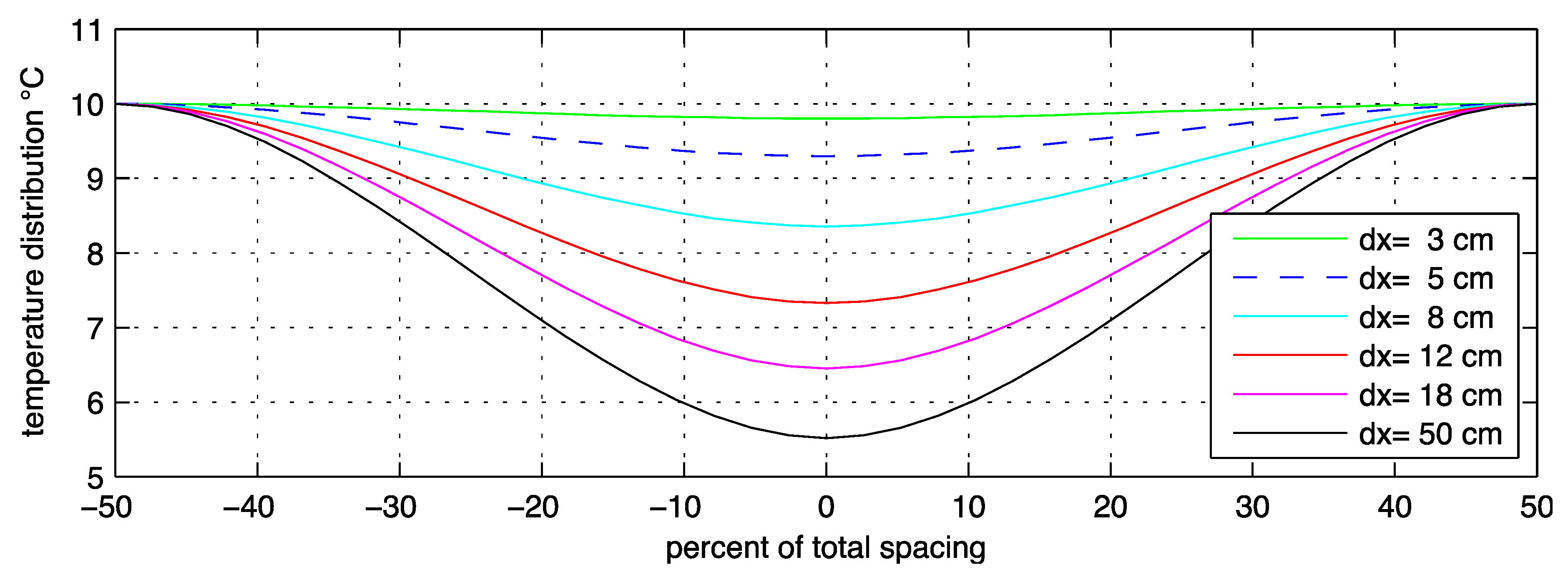
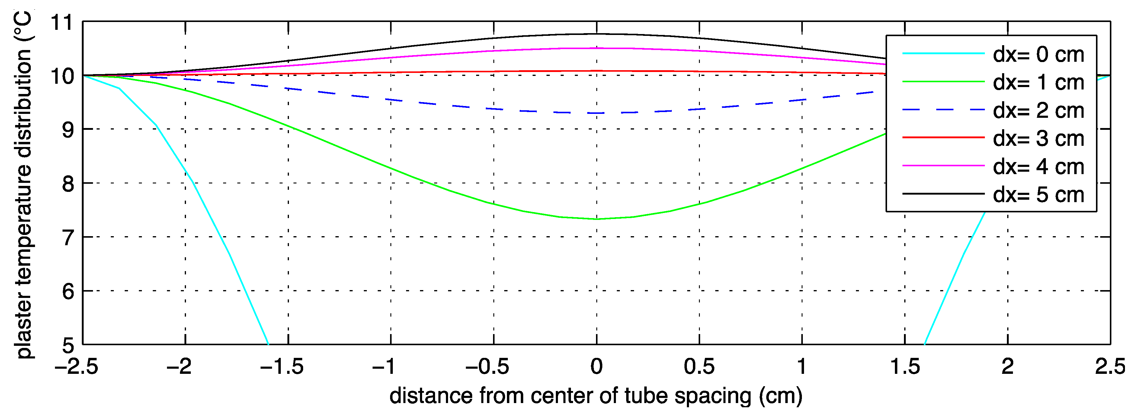
Figure 4 for the pipe spacing and the outer insulation. The pipe spacing and the amount of insulation placed on top of the piping layer determine the temperature profile, and thus the average interface temperature of the piping system and its overall performance. Therefore, the spacing and thickness were explored to determine an optimal performance that maintains a thin profile without excessive insulation, while also not requiring an excessive amount of piping to be installed. The system was analyzed at a design condition of −10 °C. This led to the base case design selection for 5 cm tube spacing and 2 cm of outside insulation. In this case, the maximum temperature deviation between the water temperature and the temperature in the middle between two tubes is 0.75 °C.
Figure 3.
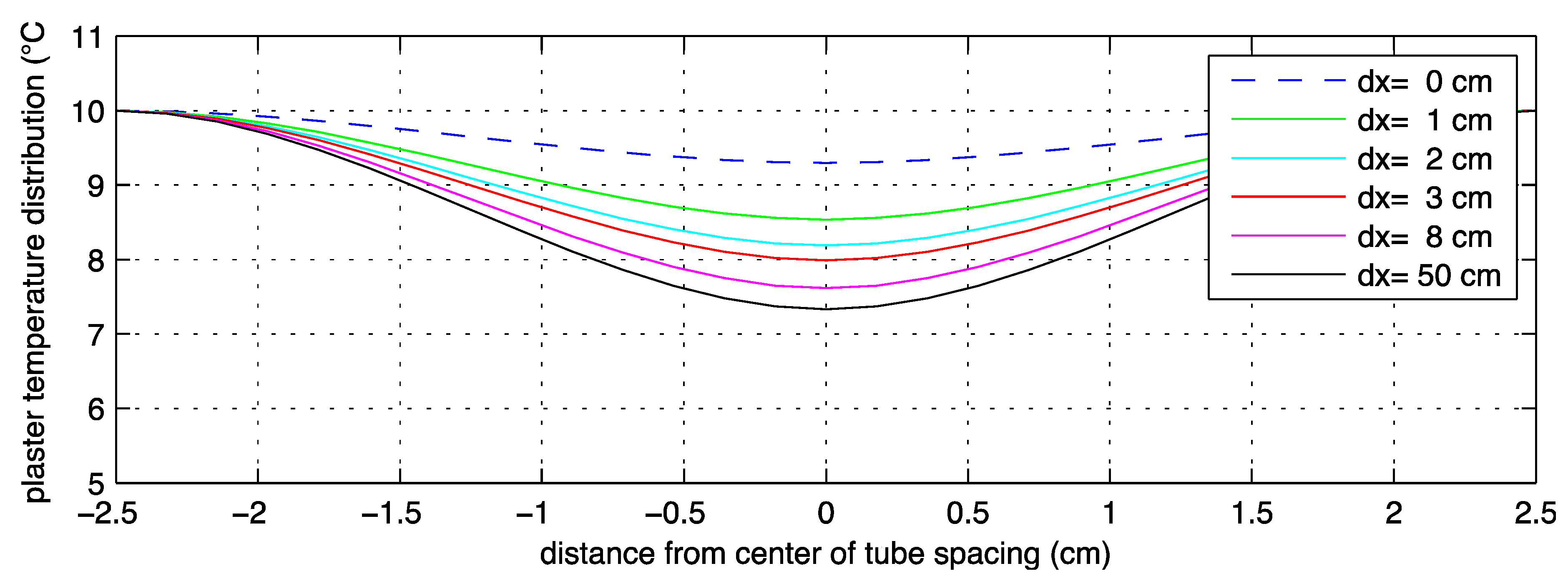
Variation of plaster temperature with different spacing (dx) of the piping in the wall. The edges of the plot represent the pipe location. The blue dashed line is the selected scenario with 5 cm spacing, keeping the change in temperature below 1 °C.
Figure 3.
Variation of plaster temperature with different spacing (dx) of the piping in the wall. The edges of the plot represent the pipe location. The blue dashed line is the selected scenario with 5 cm spacing, keeping the change in temperature below 1 °C.
Figure 4.
Variation in the temperature profile between pipes in the active layer with varying outer insulation thickness (dx). Higher amounts actually cause the layer to be heated from the inside, which means a better performance of the base wall is needed as provided by
Figure 5.
Figure 4.
Variation in the temperature profile between pipes in the active layer with varying outer insulation thickness (dx). Higher amounts actually cause the layer to be heated from the inside, which means a better performance of the base wall is needed as provided by
Figure 5.
Figure 5.
Temperature profiles for additional inner insulation. This is equivalent to having a thicker wall or a better insulating concrete. Blue line corresponds to
Figure 3 and
Figure 4 with 2 cm outer insulation and 5 cm tube spacing.
Figure 5.
Temperature profiles for additional inner insulation. This is equivalent to having a thicker wall or a better insulating concrete. Blue line corresponds to
Figure 3 and
Figure 4 with 2 cm outer insulation and 5 cm tube spacing.
Figure 4 shows that with enough outer insulation, the pipe layer actually heats up from the heat flux coming from inside the building. This means that the insulation would keep the layer at a higher temperature than the water, and so the active layer would not provide any benefit. In order to find the optimal solution the base wall should also have adequate thermal insulation for the ground temperature layer. This is explored in
Figure 5, where the influence of additional inner insulation on the temperature profile is observed. Here the temperature profile increases to a limiting value fixed by the amount of outer insulation. For the active wall system we tried to find a balance between added performance from the insulation on the inside and outside of the layer, which we explored by quantifying the equivalent static insulation in the next section of our analysis.
3.2. Equivalent Static Insulation Comparison
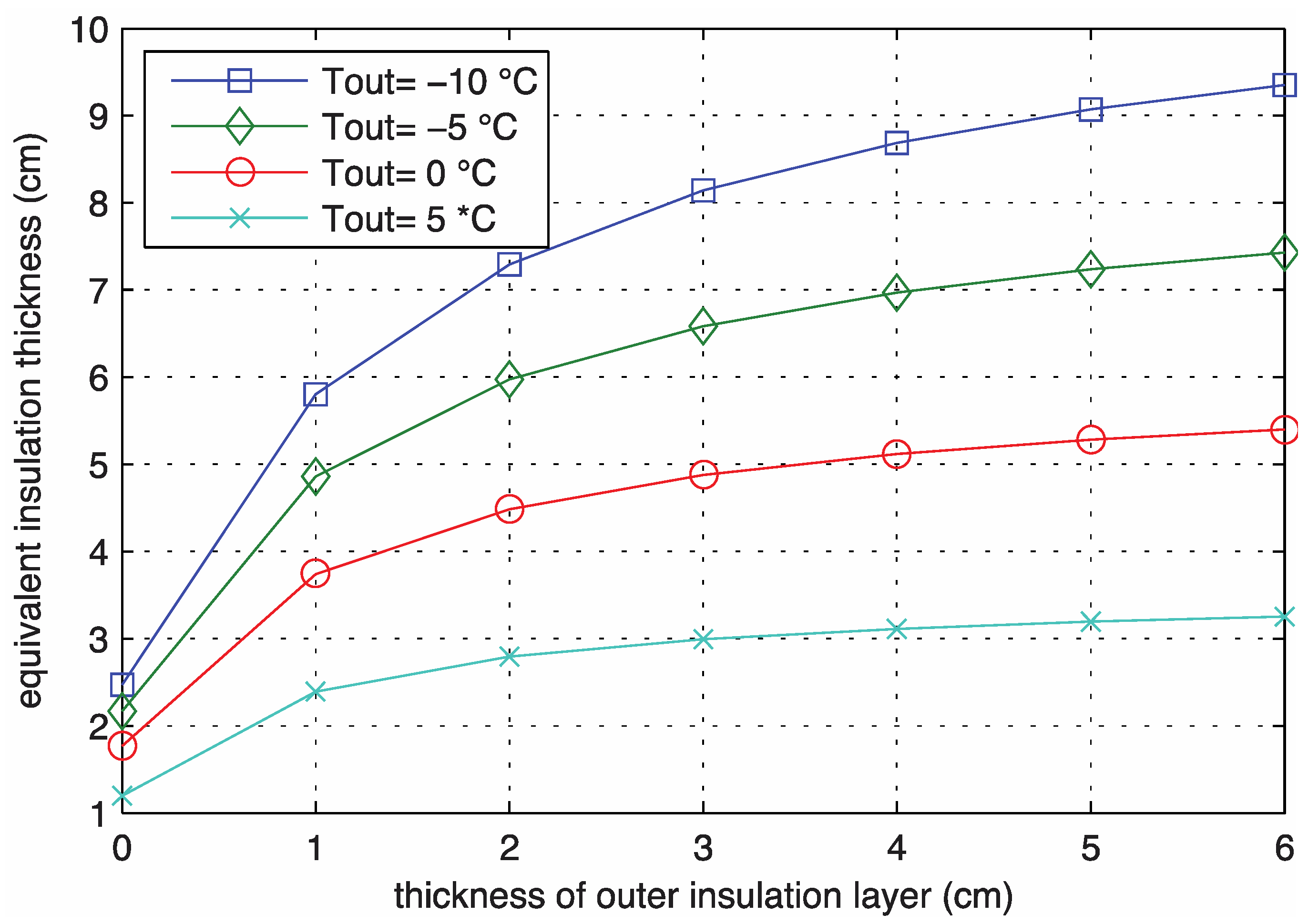
The performance of the active system has been equated to the thickness of static insulation that would be required to achieve the same heat transmission reduction. This equivalent insulation value, increases for the active system as the outside temperature decreases. Besides being dependent on the outside temperature, the performance can be influenced by design aspects of both the insulation behind and on top of the active water layer as described in
Figure 4 and
Figure 5. The insulation levels serve as design parameters whose influence on the equivalent insulation performance have been explored in
Figure 6 and
Figure 7.
Figure 6.
Variation in the equivalent static insulation thickness as a measure of the active system performance for different amounts of outer insulation for the system, assuming a base insulation layer of 2 cm.
Figure 6.
Variation in the equivalent static insulation thickness as a measure of the active system performance for different amounts of outer insulation for the system, assuming a base insulation layer of 2 cm.
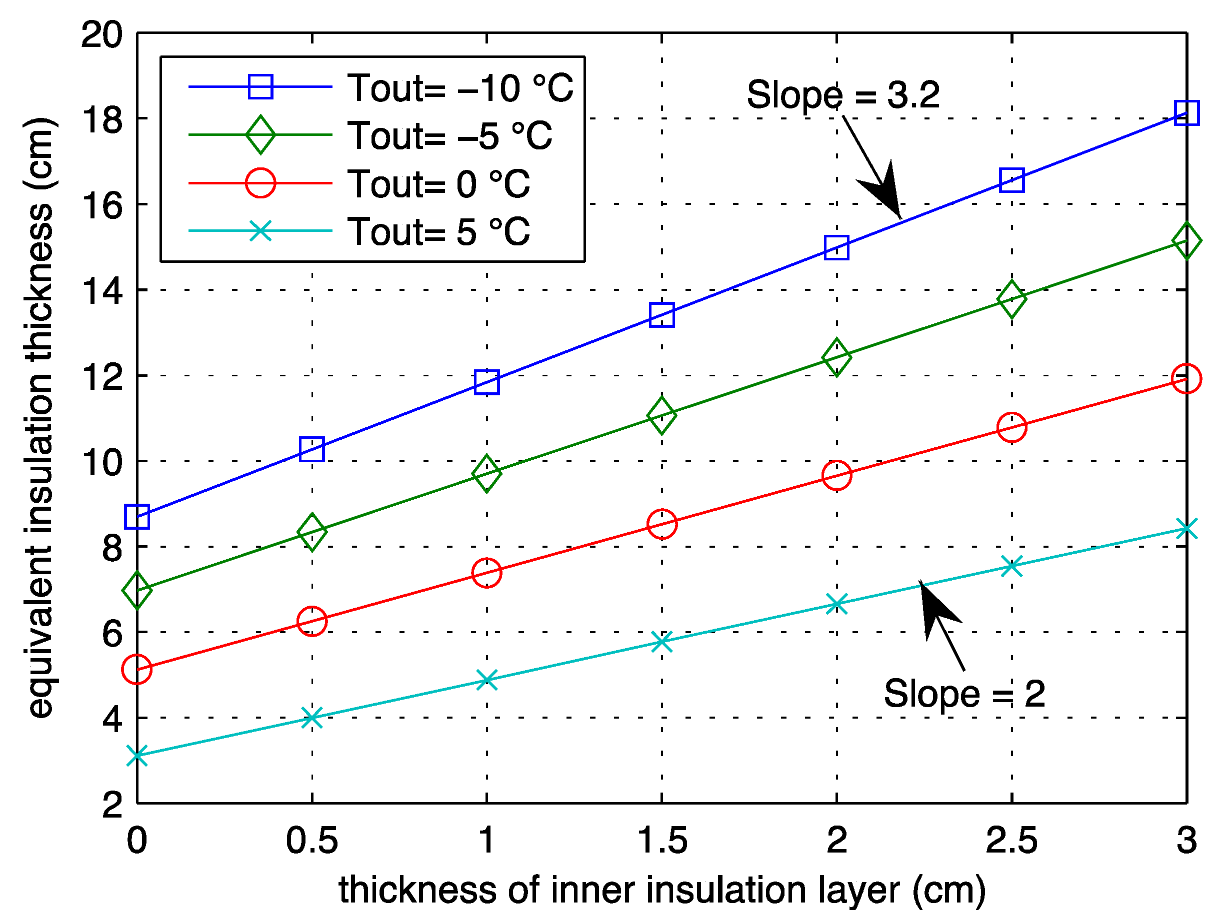
Figure 7.
Variation in the equivalent static insulation thickness as a measure of the active system performance for different amounts of inner insulation installed behind the piping layer. Here the slope or ratio of increase in equivalent insulation and inner insulation is constant and more importantly greater than one.
It is clear that the first centimeters of outer insulation are very important in achieving a good performance, but the impact is reduced as further amounts are added. Beyond 3 or 4 cm of outside insulation the increase in equivalent static insulation is less than the actual amount of outer insulation added. Nevertheless, with 2 cm of outside insulation added the equivalent insulation is >7 cm. We chose to add 2–3 cm of inner insulation to the base case after analyzing the
Figure 7.
Internal insulation is basically used to set an appropriate thermal performance of the material between the ground temperature and the inside. At 10 °C the active layer temperature still needs to be insulated from the inside to achieve a good performance and the base concrete construction is insufficient. Adding internal insulation behind the piping layer causes an expected linear increase in performance as shown in
Figure 7.
More interestingly for each cm of internal insulation added, the amount of equivalent static insulation increases by a larger factor. This ratio is caused by the fact that the temperature difference across the inner insulation added to the system is between the room temperature and the active layer temperature, whereas the value of equivalent static insulation is determined across the difference between the outside temperature and the room temperature. Therefore the ratio of these temperature differences causes the inner insulation to have a greater impact per centimeter. Adding just 3 cm of internal insulation increases the equivalent insulation thickness from 8.4 cm to 18 cm.
The internal insulation also provides a base performance level when the active system is not running. It can be seen in
Figure 6 and
Figure 7 that at the warmer outside temperature of 5 °C, the equivalent static insulation value is near the actual system thickness, making the active operation redundant. During mild conditions the system can be turned off and achieve reasonable static performance with the inner and outer insulation layers. In this way the system acts as a buffer that virtually eliminates the impact of the coldest temperatures on the heat demand of the building, while providing adequate insulation at mild temperatures.
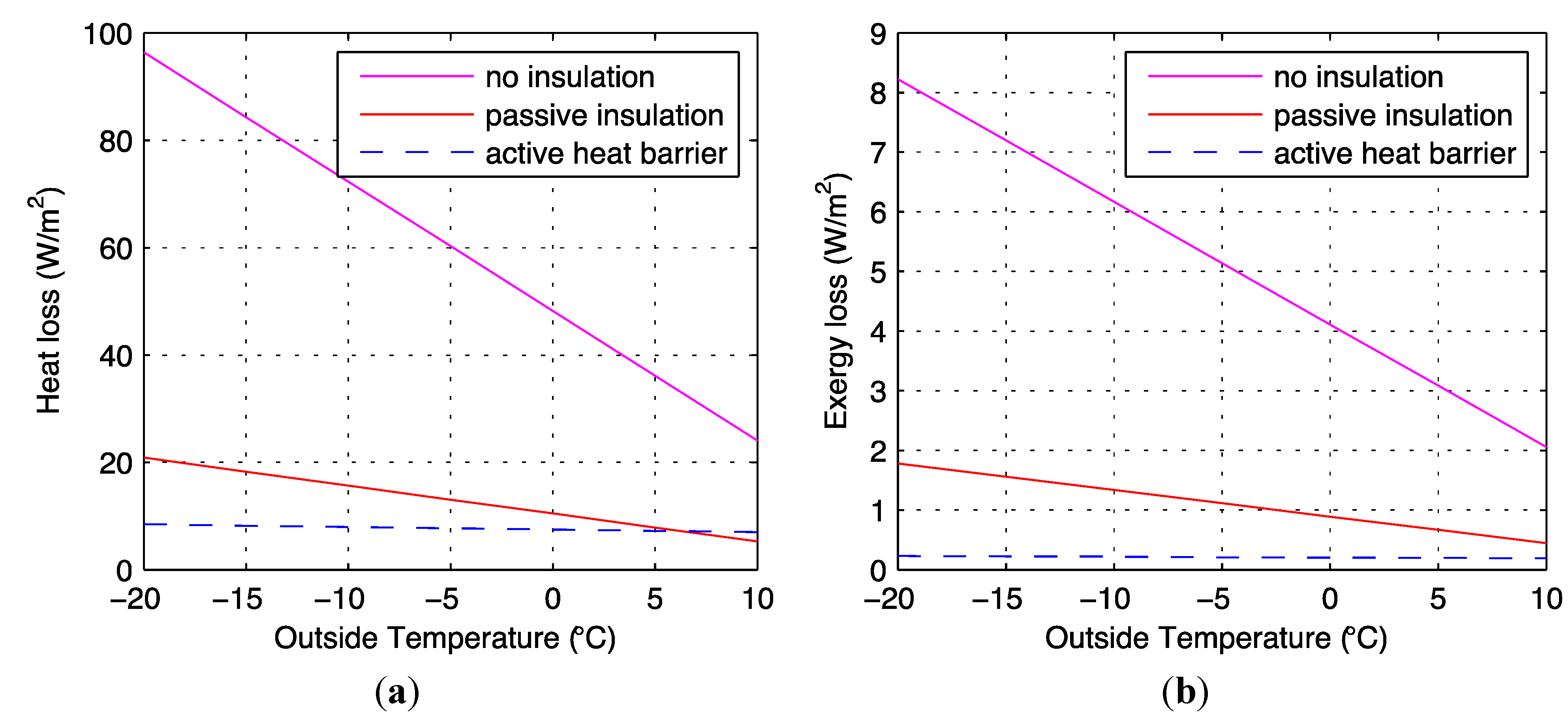
3.3. Heat and Exergy Loss Comparison
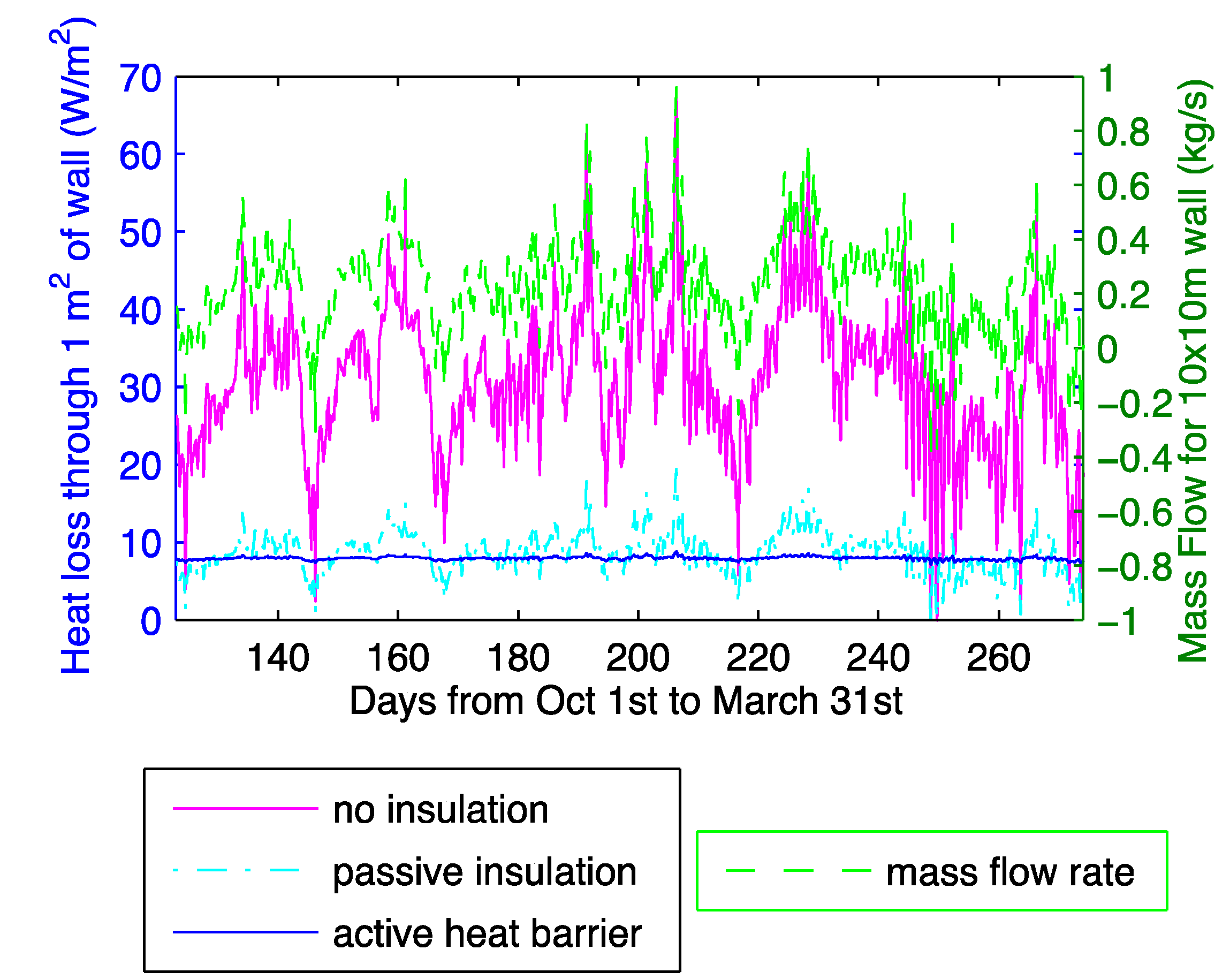
A direct comparison of the heat loss (a) and exergy loss (b) per unit area of wall are given in
Figure 8. A setup with 2 cm of outer and 3 cm of inner insulation was found to have a good performance for comparison to standard construction, and is still fairly thin. The active system is compared over a range of outside temperatures to the base construction with no insulation and to standard passive insulation 6 cm thick, equal to the active system total thickness.
The heat losses are smallest for the active insulation except for high outside temperatures where a regular static insulation of the same thickness performs better. The most remarkable property of the active insulation is apparent in the slopes of the curves. The active insulation produces a very flat, almost horizontal curve for the heat loss. This means that the heat loss becomes almost constant, independent of the outside temperature, which has the potential to improve the performance of the heat pump system as well as the lifespan because turning systems on and off or modulating components leads to more rapid deterioration.
The heat loss from the active system is less than the static insulation up until outside temperature above 7 °C. Therefore the passive insulation is better at milder temperatures, but the active system has double the performance at design conditions, and eliminates these peak demands from the system. When we consider the exergy loss from the room in
Figure 8(b), we can see how the active system exergy loss is reduced more than the others by being shifted to the ground temperature reference. We reduce the value of the air in the room by having it interact with a different part of its external environment, thereby generating the low exergy aspect of the system and helping minimize the exergy input for operation.
Figure 8.
A comparison of (a) the heat loss and (b) the exergy loss through one square meter of wall for the active insulation compared to an equivalent amount of passive insulation and the wall with no insulation.
Figure 8.
A comparison of (a) the heat loss and (b) the exergy loss through one square meter of wall for the active insulation compared to an equivalent amount of passive insulation and the wall with no insulation.
3.5. Costs and Payback
The costs as compared to a standard system have not been precisely evaluated. The additional cost will come primarily from the purchase and mounting of the piping system to the wall. This could be minimized by simplifying and mass-producing the technology in rolls similar to indoor wall-mounted capillary tube systems. The pipes could easily be draped from a large supply pipe and plastered over without much additional labor cost, and small plastic tubing can be obtained for reasonable prices. Still, simple spray-on insulation will always be less expensive, but it has limited application thickness and thus limited performance. When the performance of the active water system exceeds these limits, then the system becomes market viable because thicker more extensive insulation installations beyond spray-on plaster result in much thicker walls. They will have a comparative cost to that of the active water system. In these cases when a heat pump is installed as well, the active water wall system will be very competitive.
4. Conclusions
We have presented an analysis of the ALEGIS concept that demonstrates the feasibility of such a construction. A potential construction has been reviewed, and the performance has been compared to a similar retrofit using standard insulation.
The initial analysis of the temperature distribution between the pipes showed that a reasonable temperature distribution and average temperature could be achieved with 1 cm pipes spaced every 5 cm. For this performance the number of pipes was not insignificant, but the installation is still feasible. The amount of outer insulation needed for a good average temperature was approximately 2–3 cm.
We explored of the effects of the amounts of insulation installed below and on top of the active water layer, and compared that to the performance of static insulation. Here the results were mixed because at mild temperatures the active system, while much more complex, did not drastically outperform static insulation. On the other hand, during cold temperatures the system was capable of achieving excellent performance as compared to static insulation. For example, with 3 cm of inner insulation and 2 cm of outer insulation, the 6 cm thick system is equivalent to 11 cm of standard insulation. This is nearly double the system thickness. We also calculated the heat loss of the active system compared to a static system of the same thickness, which showed the superior performance at cold temperatures and showed that the active system is beneficial up to 7 °C, and has lower exergy loss at even higher temperatures. The active system maintains a relatively constant heat flux over varying outside temperatures, which provides added benefit to the operation of building heating systems.
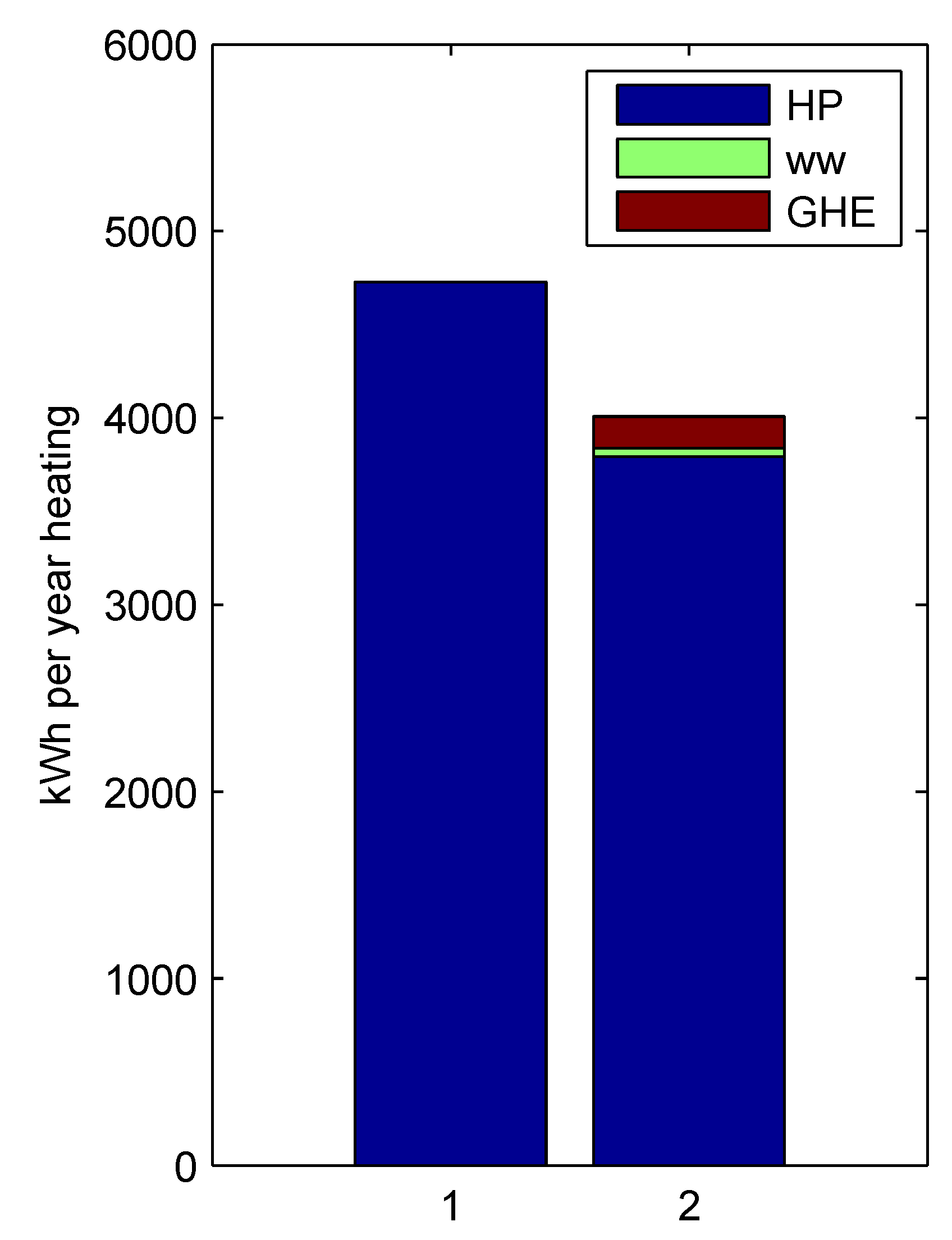
The annual performance of the system was modeled for outside temperatures for Zurich, Switzerland. The overall system performance is compared to a standard heat pump installation. The annual electricity demand is about 4000 kWh for the active system including pumping costs while a system with an equivalent amount of passive insulation (6 cm) is 15% greater at 4700 kWh. The annual electricity demand for this system is minimized with 3 cm of inner and 2 cm of outer insulation around the piping layer. This minimizes pumping costs while maximizing heat pump performance and lifespan by buffering the varying heat load from changing winter conditions.
Although several aspects of this novel building facade system have been analyzed, there are still many questions left. Further analysis and optimization may prove that for highly integrated building renovation and system retrofits, it may be the best option. More investigation into the borehole integration and heat extraction is necessary, as well as more extensive look at larger scale structures and the influence and interaction of fenestration with the system.
Nevertheless, ALEGIS provides a very novel concept for reducing heat loss from a building that provides a thinner alternative to simple standard thermally resistant insulation. We have proven it to be an interesting concept worthy of investigation. We hope that it can provide an additional tool to facilitate the reduction of exergy consumption in the building sector, especially by expanding the possibilities for performance increases through renovation and retrofit to the existing building stock.
