Article

A Phenomenological Model for Prediction Auto-Ignition and Soot Formation of Turbulent Diffusion Combustion in a High Pressure Common Rail Diesel Engine

School of Mechanical and Electronic and Automobile Engineering, Beijing University of Civil Engineering and Architecture, Beijing 100044, China
*
Author to whom correspondence should be addressed.
Energies 2011, 4(6), 894-912; https://doi.org/10.3390/en4060894
Submission received: 11 April 2011 / Revised: 5 May 2011 / Accepted: 6 May 2011 / Published: 3 June 2011
(This article belongs to the Special Issue Advancement in Combustion Sciences and Technology)

Abstract

:
A new phenomenological model, the TP (Temperature Phase) model, is presented to carry out optimization calculations for turbulent diffusion combustion in a high-pressure common rail diesel engine. Temperature is the most important parameter in the TP model, which includes two parts: an auto-ignition and a soot model. In the auto-ignition phase, different reaction mechanisms are built for different zones. For the soot model, different methods are used for different temperatures. The TP model is then implemented in KIVA code instead of original model to carry out optimization. The results of cylinder pressures, the corresponding heat release rates, and soot with variation of injection time, variation of rail pressure and variation of speed among TP model, KIVA standard model and experimental data are analyzed. The results indicate that the TP model can carry out optimization and CFD (computational fluid dynamics) and can be a useful tool to study turbulent diffusion combustion.

1. Introduction

Today’s strict emission level legislation limiting combustion-generated pollutants sets high demands on the development of cleaner engines. Since modern engines have already reached a high level of optimization through engineering measures a detailed understanding of the different processes leading to the formation of pollutants is required [1]. Soot, which is a product of incomplete combustion reducing the combustion efficiency, is identified in flames and fires as yellow luminescence and is mostly an unwanted process in today’s practical combustion devices. Soot deposits in engines or gas turbines are problematic and cause reduced efficiency, increasing the need for maintenance. Another severe problem is the effect of soot particles and their precursors on human health [2].
Due to the complexity of soot formation and the general lack of knowledge, a number of soot models have been proposed. The inception of soot particles is still not well-understood, but it is generally accepted that polycyclic aromatic hydrocarbons (PAHs) are the key soot-forming species. In the model it is assumed that the rate limiting step is the collision of two PAHs leading to the first three-dimensional structures held together by van der Waals forces. Mitchell and Frenklach [3] investigated the dynamics of agglomeration with simultaneous surface growth using a Monte Carlo method. It was found that the shape of the aggregates depends markedly on the surface growth, e.g., when surface growth is very fast the aggregates have spherical structures. To reduce the numerical demands of the method a reduction of the PAH polymerization model was proposed by Mauss [4]. Assuming that the polymerization reactions are fast or in other words, assuming that the transition from PAHs to soot is a fast process, all PAHs can be assumed to be in a steady-state. The reduction leads to an infinite system of algebraic equations describing the local PAH concentrations from which the moments of the size distribution can be calculated.
Calculations of soot formation and oxidation in diesel engines can mainly be classified into different model approaches. Balthasar et al. [5] focused mainly on the fluid dynamics of the problem using simple models for the chemical processes. Soot formation is modeled with the help of empirical or semi-empirical models. The most recent approach is based on the laminar flamelet concept, solving the so-called Representative Interactive Flamelets (RIF) on line with the CFD code. A full description of the chemical processes as well as soot and NOx formation can be obtained without having to simplify the fluid dynamics. The latter approach is the most detailed, but time consuming, and might be more difficult to incorporate into existing CFD code.
Thus, there is a need to develop numerical calculations based on accurate modeling and analysis based on the latest research results. The research presented herein focuses on obtaining an understanding of the ignition phase and soot model in a real high pressure common rail diesel engine through numerical simulations. First, a new model called Temperature Phase (TP) model is proposed, the auto-ignition phenomenon is described in some detail and implementation processes are given. Second, the experimental set-up and boundary conditions required for the calculations, as well as the operating points investigated will be discussed. Next, the simulation results and the measured data are compared. In order to assess the performance of the matching results in terms of predicting cylinder pressure and heat release over a wide range of part-load conditions, an extensive parameter study varying injection timing and rail pressure has been conducted.

2. TP Model

2.1. Auto-Ignition

2.1.1. Modified Model

Since auto-ignition is the first important event of diffusion combustion under diesel conditions, we began to construct a kinetic mechanism for n-heptane ignition based on the detailed model proposed by Barths et al. [6]. However, Barths’ mechanism (involving 324 chemical species and 1650 reactions) is too large to use in multidimensional turbulent diffusion computations. Therefore, only a few lumped or equivalent intermediate species (e.g., the first and second n-heptyl isomers were retained to represent all the n-heptyl isomers) and some relevant key reactions were selected on the basis of steady state assumptions. These reactions are crucial for reproducing the auto-ignition behavior of n-heptane/air mixtures from the low/intermediate regime to the high-temperature regime. The high temperature oxidation of n-heptane proceeds from the attack on the fuel by H, OH and HO2 radicals to form n-heptyl radicals and through the break-up of these into C2H4, CH3 and H radicals. These are oxidized by C1-C2-chemistry reactions. The low temperature chemistry of lower aliphatic hydrocarbons is characterized by the degenerate chain branching which may be illustrated by Table 1. This low temperature mechanism is no longer valid when the temperature increases beyond about 850 K. The competition of the reverse reaction of the first and second O2-addition with the subsequent internal H-abstraction reaction is the key to the understanding of the negative temperature dependence of the ignition delay. With increasing temperature, these reverse reactions become faster than their forward reactions, thereby stopping the reaction sequence. A transition to the high temperature mechanism must occur.
Table 1. Low temperature mechanism Energies 04 00894 i001.
Reactionk (1/s)nE (J/mol)
C7H16 + O2 → C7H15 + HO2 (initiation)4.500 × 10130.048810.0
C7H16 + OH → C7H15 + H2O (initiation)8.610 × 1091.101815.0
C7H15 + O2 ↔ C7H15O2 (first O2-addition)4.000 × 10120.00.0
C7H15O2 → C7H14O2H (internal H-abstraction)6.000 × 10110.020380.0
C7H14O2H + O2 → C7H14O4H (second O2-addition )6.000 × 10110.00.0
C7H14O4H → C7H14O3 + OH (chain reaction)1.000 × 1090.07480.0
The apparent negative temperature dependence of the intermediate branch shall be explained by discussing a simplified 2-step ad-hoc model with adjusted n-heptane ignition rate constants, which is shown in Table 2. A lot of parameters can be found in our previous paper [7,8,9,10]. However, at that time we only deduced and discussed these equations in theory and did not use them in a real diesel engine. Now we have used them in three-dimension turbulent diffusion combustion with turbulence movement in a diesel engine.
Table 2. Middle temperature mechanism Energies 04 00894 i001.
Reactionk (1/s)nE (J/mol)
C7H16 + 2O2 → HO2C7H13O + H2O3.500 × 10130.037810.0
HO2C7H13O + 9O2 → 7CO2 + 7H2O8.610 × 1090.01815.0
For high temperatures, we used the original KIVA-3V model [11], assuming a simplified single-step oxidation model that converts fuel and oxygen to carbon dioxide and water, because the temperature is high and reactions are very quick. We replaced the kinetic chemistry subroutine CHEM with our own specialized model.

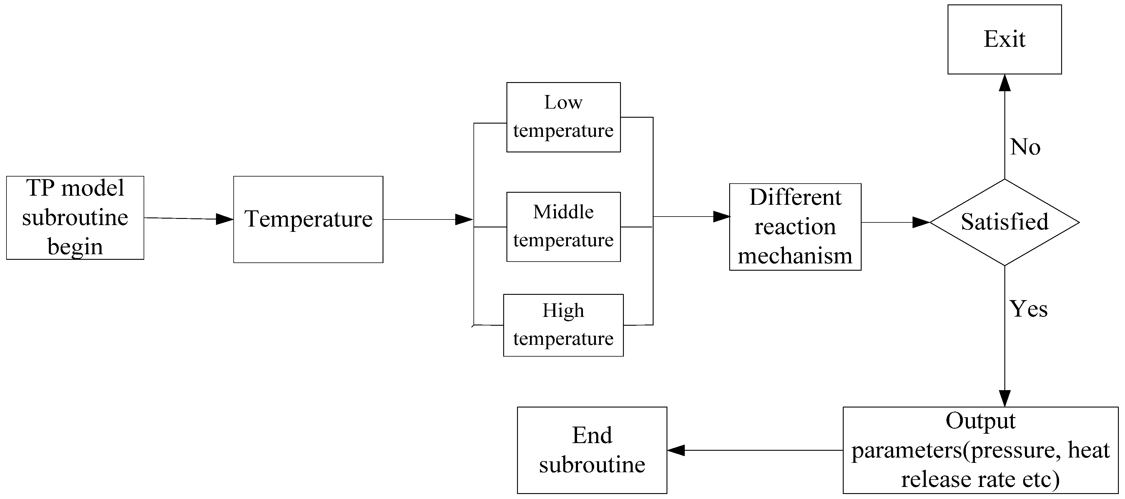
2.1.2. Implementation in CFD Code

Two steps are needed to implement the TP model in CFD code (KIVA-3V). One is making the TP model subroutine and the other is coupling the TP subroutine to the main KIVA program. The following is the description of how to achieve the above two steps:
(1) TP model subroutine
The TP model subroutine structure is shown in Figure 1. First, we select different reaction mechanisms according to different grid temperatures. When the temperature T < 850 K, we the select 6-step n-heptane model from Table 1 to calculate the auto-ignition, which explains the diesel ignition delay “S” curve in the lower part.
Figure 1. TP model subroutine structure.
Energies 04 00894 g001
When the temperature is 850 K < T < 1100 K, we select the 2-step n-heptane model from Table 2 to calculate the “S” curve in the middle of some instability. When the temperature is 1100 K < T, we use a one-step n-heptane model to calculate the upper S curve in order to save computation time. Because each grid temperature is different, we select reaction mechanisms according to each grid temperature thus avoiding all grids having the same calculation. This calculation strategy not only satisfies the original design requirements, but also greatly improves the computational efficiency. At the same time, we add a real-time control program to monitor the simulation. After each elementary chemical reaction calculation, the corresponding pressure, heat release rate, and other related information are output. If the intermediate calculations exit, it shows some parameter calculation value is divergent. The output of the calculation information is very important and it gives the scientific basis for normal calculations.
(2) Coupling TP subroutine in KIVA main program
To couple the TP model subroutine to the KIVA code, we need put it before the chem.f subroutine. The relationship between the TP subroutine and the main program is shown in Figure 2. If we want to make the TP subroutine operate smoothly, we need to calculate KIVA’s k-å turbulent movement model. Although the k-å model can provide unsatisfactory results, it can fit the calculation of the fuel injection engine. If the TP subroutine quits, we need to check the initial cylinder temperature, the cylinder pressure and other related initial data which are in the itape5 file. Because KIVA-3V can only recognize regular hexahedron shaped grids, we need to constantly adjust the establishment of x, y, z grid layers in three directions to ensure the normal calculation.
Figure 2. Relationship between TP subroutine and KIVA main program.
Energies 04 00894 g002

2.2. Soot Model

The modified soot model includes two parts: the PAH and the soot source term. The soot model used in the calculations relies on a detailed description of the chemical processes leading from the fuel molecules to complex soot particles based on the statistical momentum approach. It can be subdivided into the growth of polycyclic aromatic hydrocarbons (PAHs) in the gas phase reactions and the processes of particle inception, condensation, surface growth, and oxidation.

2.2.1. PAH Calculation

According to recent literature [12] a “skeleton” reaction mechanism plays a major role in the PAH soot precursor whereby the material (C2H2 and C4H5) is the basis for reactions to form the first benzene ring through the “add-dehydrogenation-acetylene” mechanism of the C10H8 representation of PAH components. The C10H8 oxidation product is not CO2, but CO and HC. The PAH model calculation is a modified Frenklach-Mauss fuel pyrolysis model [13] of the formation of the first benzene ring, cyclization and oxidation, whose units are seconds (s), centimeters (cm), Kelvin (K), and mole (mol).
(1) Fuel pyrolysis
First of all pyrolysis of hydrocarbon fuels occurs at high temperature to produce a variety of groups of small molecules, such as CH3, C2H2, C4H2 and C4H5, etc. In this paper, using n-heptane as the diesel calculation model, the pyrolysis equation can be written as follows:
Energies 04 00894 i002
(2) The formation of the first benzene ring
Based on the pyrolysis of fuel through acetylene (C2H2) and C4H5 the equation for the first aromatic (benzene) ring formation reaction is:
Energies 04 00894 i003
(3) Cyclization
The formation of a single benzene ring will be followed by the so-called HACA mechanism for the formation of aromatic molecules. HACA (H-Abstraction, C2H2-Addition) means that the hydrogen atom desorption from the addition of phenyl acetylene molecules, referred to as “plus-acetylene- dehydrogenation” mechanism, but this calculation is different from the FM in the detailed model, using literature [14] in the test results. Using naphthalene (C10H8, abbreviated as A2, i.e., an aromatic hydrocarbon with two benzenes) as the PAH the representation of the nuclear components during the chemical reaction is as follows:
Energies 04 00894 i004
Energies 04 00894 i005
(4) PAH growth, rapid polymerization and oxidation
PAH growth in the early stages mainly produces planar structures. Due to the special stability of certain aromatic components, it is difficult for the reverse reactions to occur, so these rings involving accumulation of hydrocarbon molecules will grow rapidly. Of course, this growth will not be unlimited, because at the same time, an opposite process occurs, namely the oxidation of hydrocarbons, so the growth of PAHs is inhibited after growth exceeds more than four PAH rings. Growth continues by relying on the so-called “linear heap together” approach (linear lumping technique), and its principles are still based on HACA. However, due to the involvement of OH and O and PAH-generated reactive species in chemical reactions, and the presence of some reverse reactions, the formation and consumption of PAH between the two processes reaches a certain “balance”. PAHs inhibit the growth of lean combustion processes and taking into account the oxygen-rich state in the linear stack PAH accumulation process, the introduction of OH and O2 causes oxidation. As the OH-based oxygen activation energy activation energy is only 2/3 that of O2, OH is a more effective oxidant than oxygen. The PAH oxidation product is not CO2, but rather CO and HCs, and the corresponding chemical equation is:
Energies 04 00894 i006

2.2.2. Soot Source Term

The formation of soot can be subdivided into the processes of particle inception, surface growth, oxidation and coagulation.
(1) Particle inception
In the present study, we have followed the work of Tao and Golovitchev’s, and assume that soot particle nucleation takes place at sites where diacetylene (C4H2) or naphthalene (A2) exist. The choice of these two species is based on the argument that soot particle nucleation is not merely linked to the pyrolysis of the hydrocarbon fuel, as assumed by Lindstedt [15], but it also has its own, unique macro-molecular precursor formation chemistry. Strictly speaking, however, these two reaction steps do not represent the soot particle nucleation process correctly, because soot does not only contain carbon atoms in its incipient particles, but also considerable amounts of hydrogen. In addition, there are uncertainties regarding the determination of the rate constants of these two reactions. As will be shown below, the values of the effective activation temperature for soot nucleation used in Lindstedt’s model are too high for use in the present study. Unless a very high pre-exponential factor is employed, computations with Lindstedt’s nucleation model predict a rather low soot mass concentration. We have found that appropriate values for the effective activation temperature are below 5000 K, thus we assign a value of 1500 K for this parameter in the present study because it provides reasonable predictions compared with the available experimental data, especially for the short time available for soot formation immediately after ignition. Initiation of the process of soot and hydrocarbon fuels is not only related to the thermal solution, but also with a specific precursor-related chemical processes. Results show [16,17], that flame and carbon-related intermediate species, mainly PAH and polyacetylene, play an equally important role in soot particle nucleation, which would follow Equations (6) and (7):
C10H8 → 10Csoot + 4H2
C4H2 → 4Csoot + H2
kA2 = kC4H2 = 1.0 × 10⁷ exp(−5000/RT)
Both the total package reaction to remove a large number of intermediate species and reaction details will reduce the computation time, but also provides a determined carbon grain initial surface area and a simple way to follow-up on the surface growth and particle number density of the initial calculations. Based on these two reactions, it is easy to write the soot nucleation rate formula:
ωNu = 10kA2[A2] + 4kC4H2[C4H2]
(2) Surface growth
We have adopted the idea of Frenklach and Wang’s active site model [18] for the present study. However, the model was modified by the inclusion of the irreversible reaction to account for the activation of surface sites by OH radicals and the deactivation of surface radical sites by H2O. This reaction is found to be critical in the soot formation in diesel spray combustion and the rate constants are fully consistent with those of the HACA reactions of PAHs. Only part of the rate constant for reaction is adjusted, to achieve agreement with experimental data.
(3) Surface oxidation
Soot oxidation is a heterogeneous process that takes place on the surface of soot particles and depletes the carbon atoms accumulated in the particles. However, since the mechanism of this process is still poorly understood, it is commonly described using empirical formulations such as the Nagle and Strickland-Constable semi-empirical model to account for soot oxidation caused by O2 attack. This model is adopted in the present study. The soot oxidation is also sensitive to other oxidants such as OH radicals. We include Neoh et al.’s OH oxidation model and the rate, correlated to the collision efficiency of OH radicals with the soot surface.
(4) Particle coagulation
Particle coagulation causes the number of soot particles to decrease. We assume a monodisperse size distribution of the particles, and then describe the coagulation by the Smoluchowski equation.
(5) Soot Source Terms
The formation of soot can be subdivided into the processes of particle inception, surface growth and oxidation, particle coagulation. For the PAHs a statistical approach is used to describe the size distribution function of the soot particles. The moments of the size distribution of the size are defined as:
Energies 04 00894 i007
where Ni is the number density of particle i with a mass mi = i · m1, with m1 being the mass of the smallest unit occurring in a soot particle. The moment M0 is equal to the total particle number density:
Energies 04 00894 i008
The moment M1 can be related to the volume fraction, which defines the ratio of the volume occupied by soot particles to the gas volume:
Energies 04 00894 i009
where ρs = 1800 kg/m3 is the density of soot.
The source term Mr is:
Energies 04 00894 i010
with pb = particle inception, con = condensation, sg = surface growth, ox = oxidation.
Particle inception can be modeled as the coagulation of two PAH-molecules. Coagulation of particles of the same type can be described by Smoluchowski’s equation:
Energies 04 00894 i011
This equation gives the change of the particle number in size-class i as a function of time. The first terms in Equation (13) describes the formation of new particles from smaller sized particles and the second terms the consumption of particles in the i-th size-class by coagulation with particles of all size classes. The frequency factor in the free molecular regime is given by:
Energies 04 00894 i012
where kB is the Boitzmann constant, μi,j is the reduced mass, ri is the radius of particles of class i and εi,j is the size dependent coagulation enhancement factor due to attractive or repulsive forces between the particles. The Smoluchowiski equation can be formulated for the particle inception omitting the second terms:
Energies 04 00894 i013
Equation (15) can be described in terms of the moments of the PAH size distribution by multiplying with ir and a summation over all size classes (note the change of the upper summation limit with respect to j):
Energies 04 00894 i014
One can rewrite (7) with the help of Vi = mi/ñs = i × m1/ñs:
Energies 04 00894 i015
with:
Energies 04 00894 i016
where Vi and mi are the volume and mass of particle of size class i respectively, and εi,j the coagulation enhancement due to inter-particle forces. The enhancement factor due to van der Waals interaction is set to a constant value of 2.2. The mean soot particle diameter is given by:
Energies 04 00894 i017
Tao’s experiment involved a conventional heavy-duty DI diesel engine based on injection conditions. Sandia National Laboratories reproduced the experiment in the optical engine using similar operating conditions. There are many advantages than DEC [19,20,21] conceptual model, particularly in the liquid spray penetration, fuel vapor permeability, flame structure and soot concentration on the spatial correlation. Tao et al. knew, when the larger soot particles are in fuel-rich vortex downstream of the head region, there is a thin layer of a large concentration of soot particles in the very low quality flame of the external surface area. They gave many valuable details in soot formation (for example, particle size, and density, form the material before, and acetylene concentration) and response speed (for example, the formation of soot particle coagulation, surface generation, and oxidation).

3. Simulations

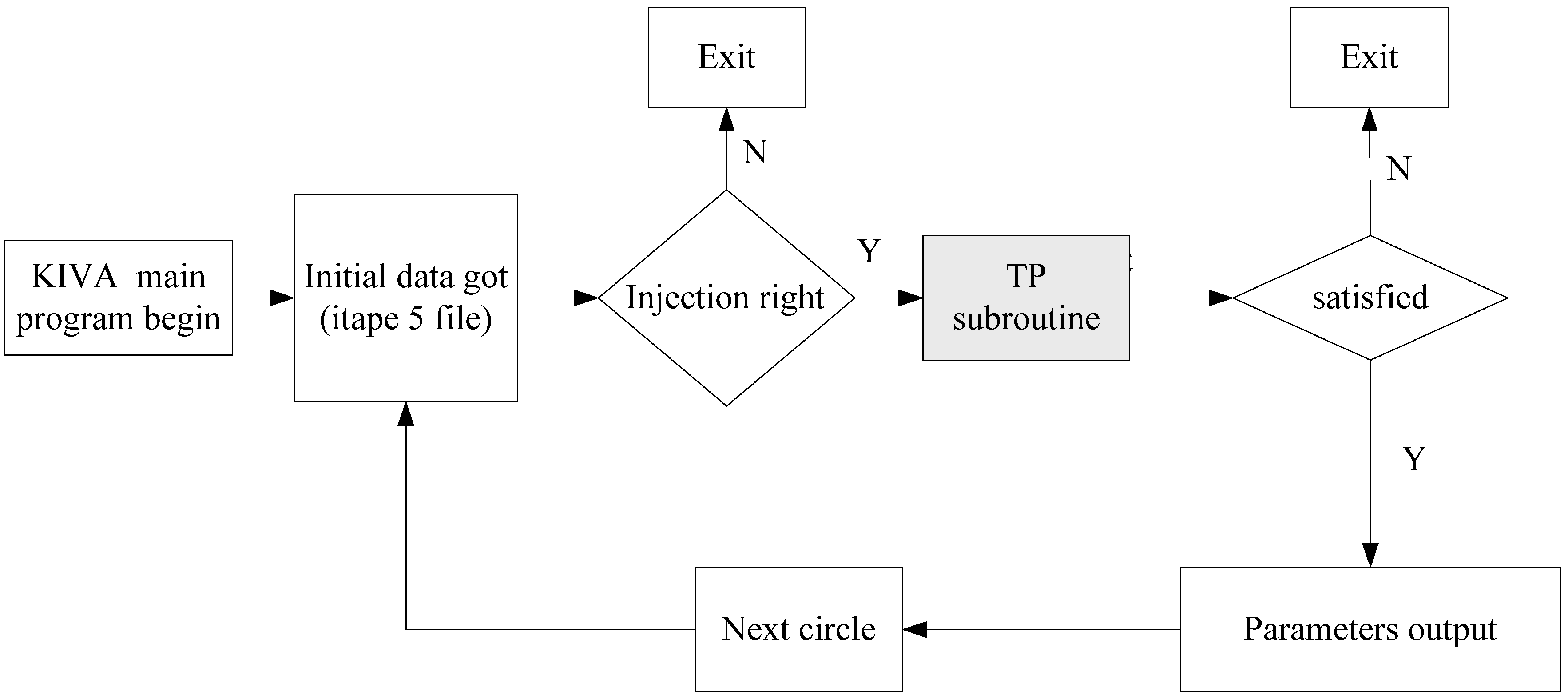
3.1. Numerical Implementation

The KIVA-3V code is used to solve the time-dependent conservation equations of total mass, momentum, energy, and species mass concentrations in the reacting gas-phase mixture. Spray dynamics are modeled using the discrete-particle technique, in which each computational particle represents a number of droplets of identical size, velocity, etc. In addition to particle-turbulence interaction, spray atomization, droplet breakup, evaporation, collision and coalescence are treated using spray sub-models for a single-component, vaporizing fuel sprays are provided in the original KIVA-3V code. Turbulence modeling is based on the compressible k-ε model (accounting for dilatation effects) modified to include the effects of fuel droplets. A characteristic micro-mixing time scale is determined from the turbulence modeling and then further used for the chemistry-turbulence interaction. All these sub-models implemented in the KIVA-3V code have been proven relevant to the accurate simulation of diesel spray combustion.

3.2. Basis for the Numerical Simulation

The computations started at IVC and ended at EVO. The injection time unit from us to CAD (crank angle degree) can use the following form for a 4-stroke engine:
Energies 04 00894 i018
where φ is crank angle degree, n is speed (r/min), t is time (μs).
The wall temperature (450 K) was set such that calculated and measured pressures matched during the compression phase before injection started. The wall temperature was held constant during the computations. The swirl was set to 0.5 times the number of revolution of the engine (r/min) which corresponds to the measured swirl. The injection nozzle was located on the axis of symmetry. Since the shape of the piston is not on the axis of symmetry, 360° was modeled which corresponds to x-offset 4 mm and y-offset 1 mm. This made the model 360-degrees, offering exact calculation of the full geometry. Figure 3 shows the computational grid used in the simulations containing 204,000 cells.

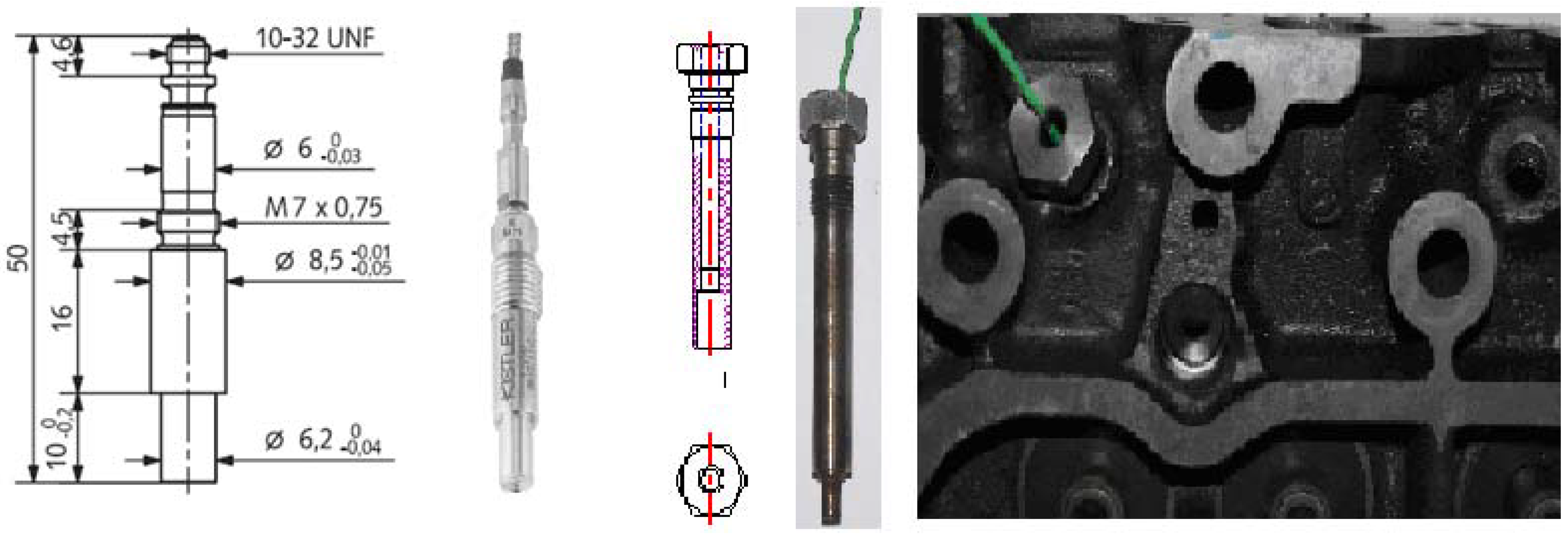
3.3. Experiment Set-up

In the process of engine bench tests, the cylinder pressure must be strictly monitored for the various tanks, therefore, the cylinder head design needs to be modified with the four warm-plugs and the cylinder pressure sensor is installed on the transition casing. Figure 4 is the cylinder pressure sensor design and structure. The in-cylinder pressure was measured using a flush mounted quartz sensor from Kistler (type 6061B).
Figure 3. Computational grid used in the simulations.
Energies 04 00894 g003
Figure 4. Cylinder pressure sensor structure and design.
Energies 04 00894 g004
The pressure transducer is very accurate on a relative basis but does not directly yield absolute values. In this measurement, the reference was taken to be atmospheric pressure and it had to be corrected for the applied boost pressure. The peak motored cylinder pressure is extremely sensitive to small changes in the pressure at intake valve closing (IVC).
Figure 5 shows a schematic of the test bench configuration. The test engine is a four cylinder, 2.8 L 4JB1 DI engine. Bore is 93 mm, and stroke is 102 mm. Swirl ratio is 2.4. Compression ratio is 18.2. Connecting rod is 168 mm. Injector protrusion is 1 mm. The injection system is a third generation Bosch Common-Rail featuring a maximum injection pressure of 2500 bar. The injector is equipped with a six-hole nozzle, where each hole has a diameter of 0.124 mm. Soot was measured with the ELPI (Electrical Low Pressure Impaction). The ELPI is a real-time particle size spectrometer designed at the Tampere University of Technology for real-time monitoring of aerosol particle size distribution. The ELPI measures airborne particle size distribution in the size range 0.03−10 µm with 12 channels. With a filter stage the size range can be extended down to 7 nm. The operating principle is based on particle charging, inertial classification in a cascade impaction, and electrical detection of the aerosol particles. The main components of the instrument are a corona charger, low-pressure cascade impaction and multi-channel electrometer.
Figure 5. Schematic of the experimental set-up.
Energies 04 00894 g005
Table 3 summarizes the relevant 4JB1 engine operating data for the 13 load conditions of the European Stationary Cycle (ESC) Since the Euro III standard (2000), the earlier steady-state engine test ECER-49 has been replaced by two cycles: the ESC and the European Transient Cycle (ETC). Smoke opacity is measured on the European Load Response (ELR) test. The following testing requirements apply for Compression ignition diesel engines: (1) Euro III: Conventional diesel engines: ESC/ELR test, Diesel engines with “advanced after-treatment” (NOx after-treatment or DPFs) and EEVs: ESC/ELR + ETC; (2) Euro IV and later: ESC/ELR + ETC. ESC is the basic requirement for Euro III and Euro IV but here we discuss only one work condition due to the size limitations of this paper. The investigated load conditions are 2200 r/min, 25% load, 50% load and 75% load, and 2700 r/min, 75% load are from 13 work conditions which include different speeds, different torques and different rail pressures. Previous investigations have shown that the load predictions part represents a particularly challenging modeling task [22]. The injector is slightly offset (by 1.0 mm) to the center of the cylinder axis to allow a better cooling of the narrow bridge between the exhaust valves. Whereas the engine experiments were performed using standard diesel fuel, a model fuel comprising n-heptane was used to represent diesel in the simulation. Rutland et al. showed that the model fuel displays very similar performance and emission characteristics to diesel.
An important input for the spray calculation is the injection rate profile. In this study, the fourth generations of EFS 8420 France products was used for consistency of measurement, reproducibility, responsiveness, the ability to spray twice for the assessment of its verification aspects. In order to accurately measure the volume of a single injection, we need to set the nozzle back pressure in the external environment, usually to 20 bar, when the back pressure built up and stabilized at around 20 bar rear pressure can be measured. Four generations of products in terms of injection rate measurement principle, monitor friendly interfaces, operability, and so the two jet measurement capabilities are greater than the three generations of product improvements, the fuel injection quantity per injection can be a data output, injection rate curves can be displayed in real-time monitoring software, very intuitive, and the injection rate curve can be in picture or data format to facilitate subsequent data analysis. Figure 6 shows the measured injection rate profiles corresponding to rail pressures of 723 bar, 809 bar, 980 bar and 1190 bar, respectively. These shapes were used as input for the simulations to be presented.
Table 3. The thirteen work conditions of ESC.
Speed (r/min)Torque (N.m)Power (kW)Rail Pressure (bar)
750 (Idle)00330
2200 (100% load)27664.4241200
2200 (75% load)21149.23980
2200 (50% load)13531.498809
2200 (25% load)6414.926723
2700 (100% load)25071.3671200
2700 (75% load)19553.3631190
2700 (50% load)12736.241900
2700 (25% load)6418.256750
3200 (100% load)23981.5921300
3200 (75% load)17961.1081200
3200 (50% load)12141.3081100
3200 (25% load)5920.1361000
Figure 6. Injection rate profile. (A) Rail pressures at 723 bar; (B) rail pressures at 809 bar; (C) rail pressures at 980 bar; (D) rail pressures at 1190 bar.
Energies 04 00894 g006

4. Results and Discussion

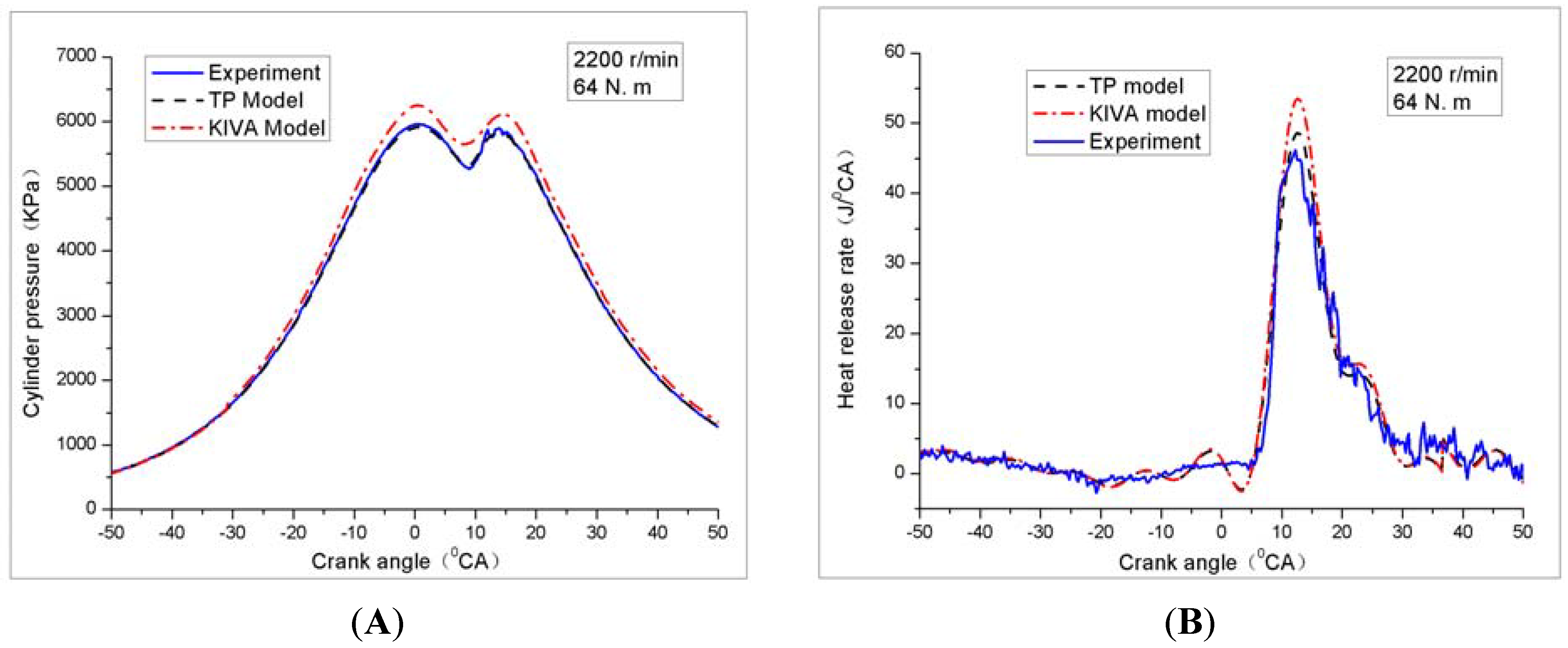
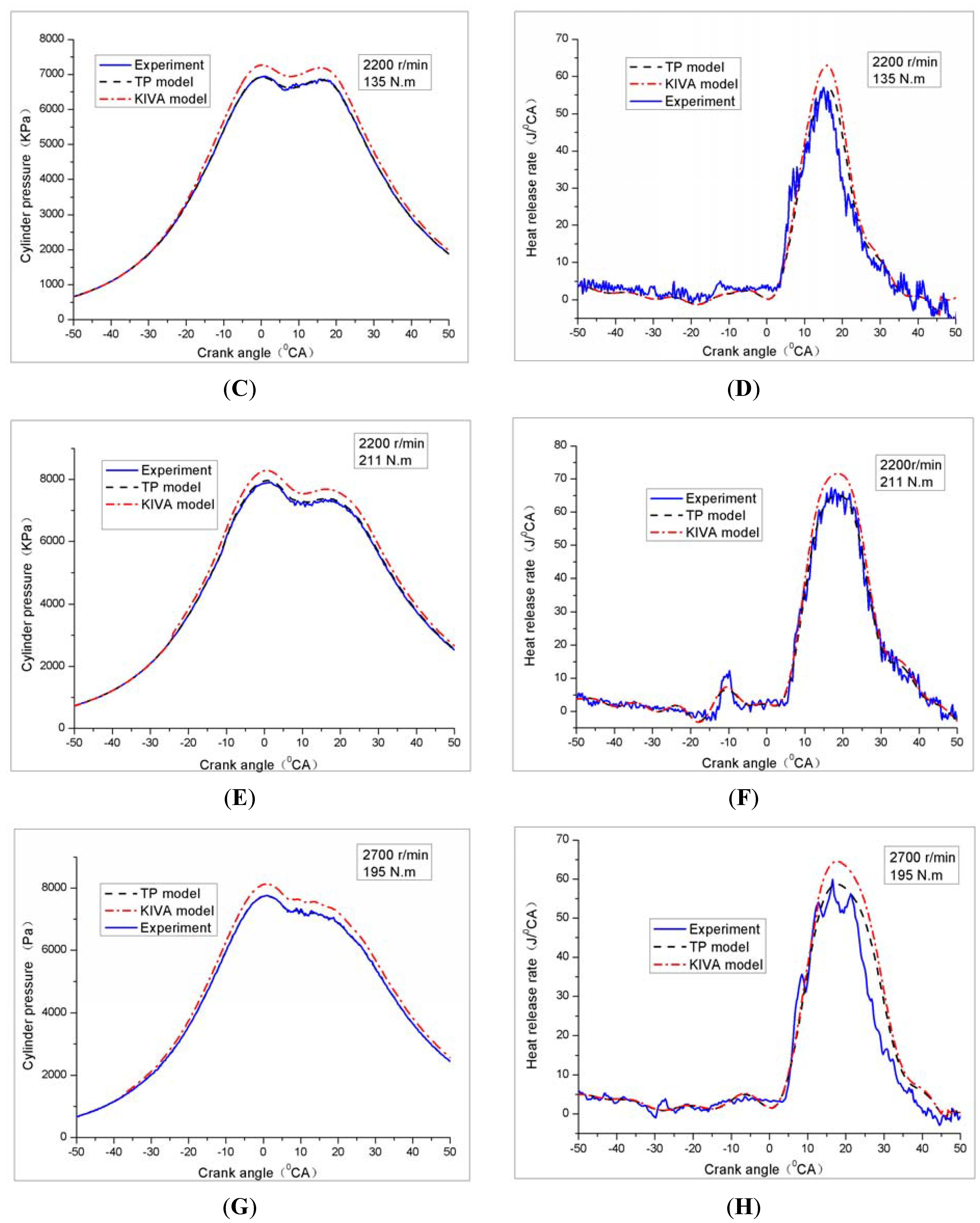
4.1. Cylinder Pressure and Heat Release Rate

For each of the simulations cylinder pressure and heat release rate are compared with measured values. Figure 7 shows the cylinder pressure traces and corresponding heat release rates for the measured and simulated parameter study varying the work conditions. As can be seen in Figure 4, the overall agreement in both ignition delay and peak cylinder pressure are excellent. For 2200 r/min 64 Nm, the cylinder pressure is changed quickly when it is 20 °CA (Crank angle) BTDC (before top dead center). So the ignition delay time is 12°CA. The biggest experimental pressure is 5800 KPa, which is near to TP model (5820 KPa) and far from KIVA original model (6020 KPa). The heat release rates are similar between TP model (45 J/°CA) and experiment (42 J/°CA), but in the original KIVA model it is 55 J/°CA. This is due to fact the TP model is a multi-step chemistry model and KIVA is a one step model. But the difference between the original model and the improved model decreases with the fuel injection quantity, because as the fuel injection quantity increases, power increases, the cylinder temperature and pressure increase and the difference between the multi-step and one step models decreases. The cylinder pressures are well fitted between simulation and experiment for all other work conditions. The simulation heat release rates are higher than the experiments because of different calculation steps, but the errors are small and the TP model can be used for simulating a real diesel engine.
Figure 7. Cylinder pressure and heat release rate. (A) cylinder pressure at 2200 r/min, 64 Nm; (B) heat release rates at 2200 r/min, 64 Nm; (C) cylinder pressure at 2200 r/min, 135 Nm; (D) heat release rates at 2200 r/min, 135 Nm; (E) cylinder pressure at 2200 r/min, 211 Nm; (F) heat release rates at 2200 r/min, 211 Nm; (G) cylinder pressure at 2700 r/min, 195 Nm; (H) heat release rates at 2700 r/min, 195 Nm.
Energies 04 00894 g007aEnergies 04 00894 g007b

4.2. Soot

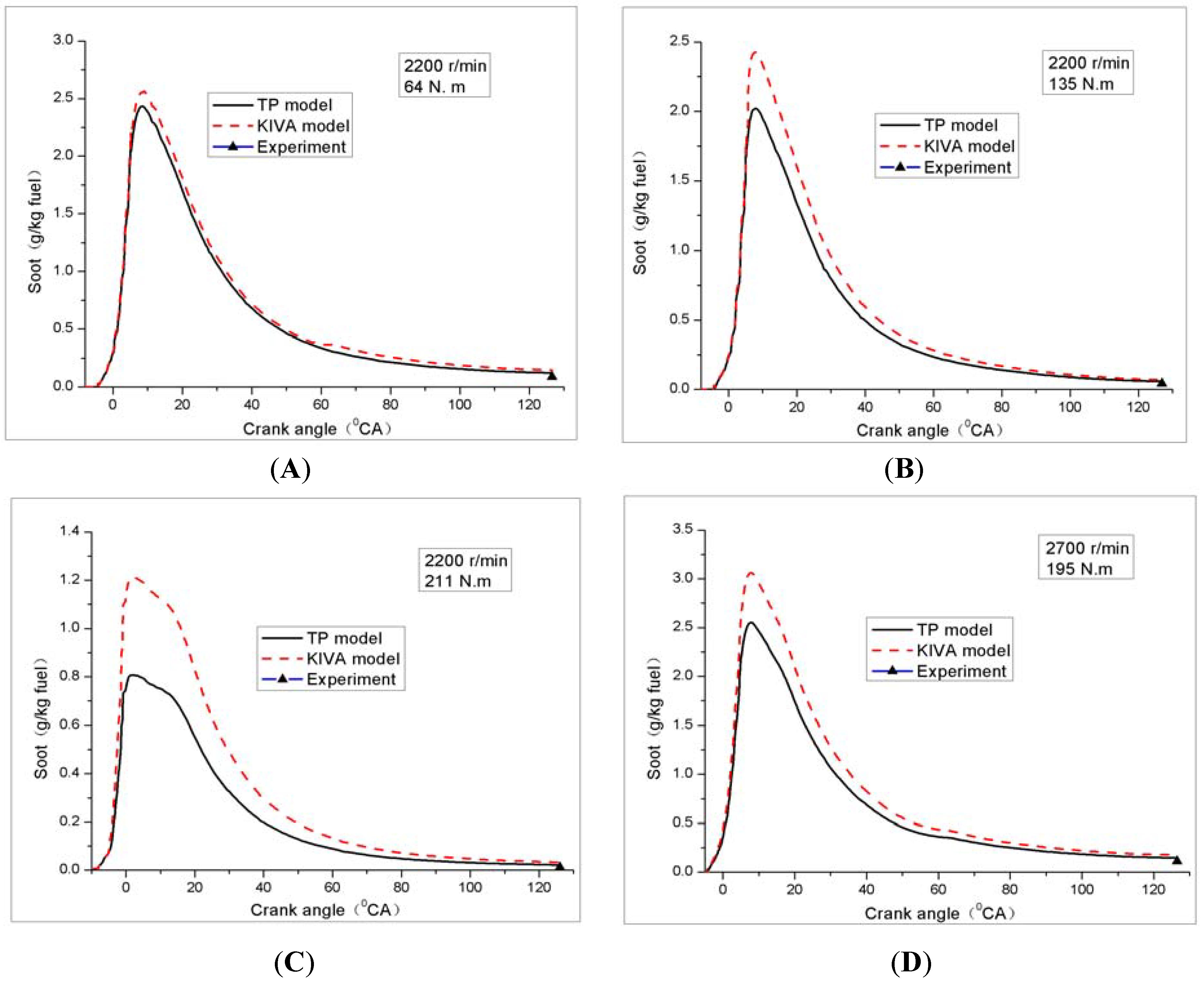
4.2.1. Soot versus Crank Angle

Figure 8 displays soot in the original model and the improved model of the development process of the cylinder. When the engine is at 2200 r/min and 135 Nm, the maximum soot value is 2.4 g/kg fuel at 8°CA ATDC and 0.12 g/kg fuel by the improved model, different from the 2.55 g/kg fuel and 0.14 g/kg fuel by the original model. The experimental value is 0.09 g/kg fuel. This shows the improved model is nearer to the experimental result than the original model. If we use the original model, the maximum soot value is 2.57 g/kg fuel at 3°CA TDC. There is 1°CA difference between the original model and the improved model, which is in line with numerous papers [23,24,25]. When the engine is at 2200 r/min and 135 Nm, the maximum soot occurs after 7°CA TDC with 2.02 g/kg fuel by the improved model and the final soot is 0.0577 g/kg fuel. The peak soot is also at this point according to the original model, but the peak value is 2.42 g/kg fuel with final generation 0.0692 g/kg fuel. The experimental value is 0.041 g/kg fuel.
Figure 8. Soot versus crank angle. (A) Soot versus at 2200 r/min, 64 Nm; (B) Soot versus at 2200 r/min, 135 Nm; (C) Soot versus at 2200 r/min, 211 Nm; (D) Soot versus at 2700 r/min, 195 Nm.
Energies 04 00894 g008
The final soot by the improved model is lower than by the original model but closer to the experimental. The improved accuracy was about 25%. This behavior has been observed under other conditions.

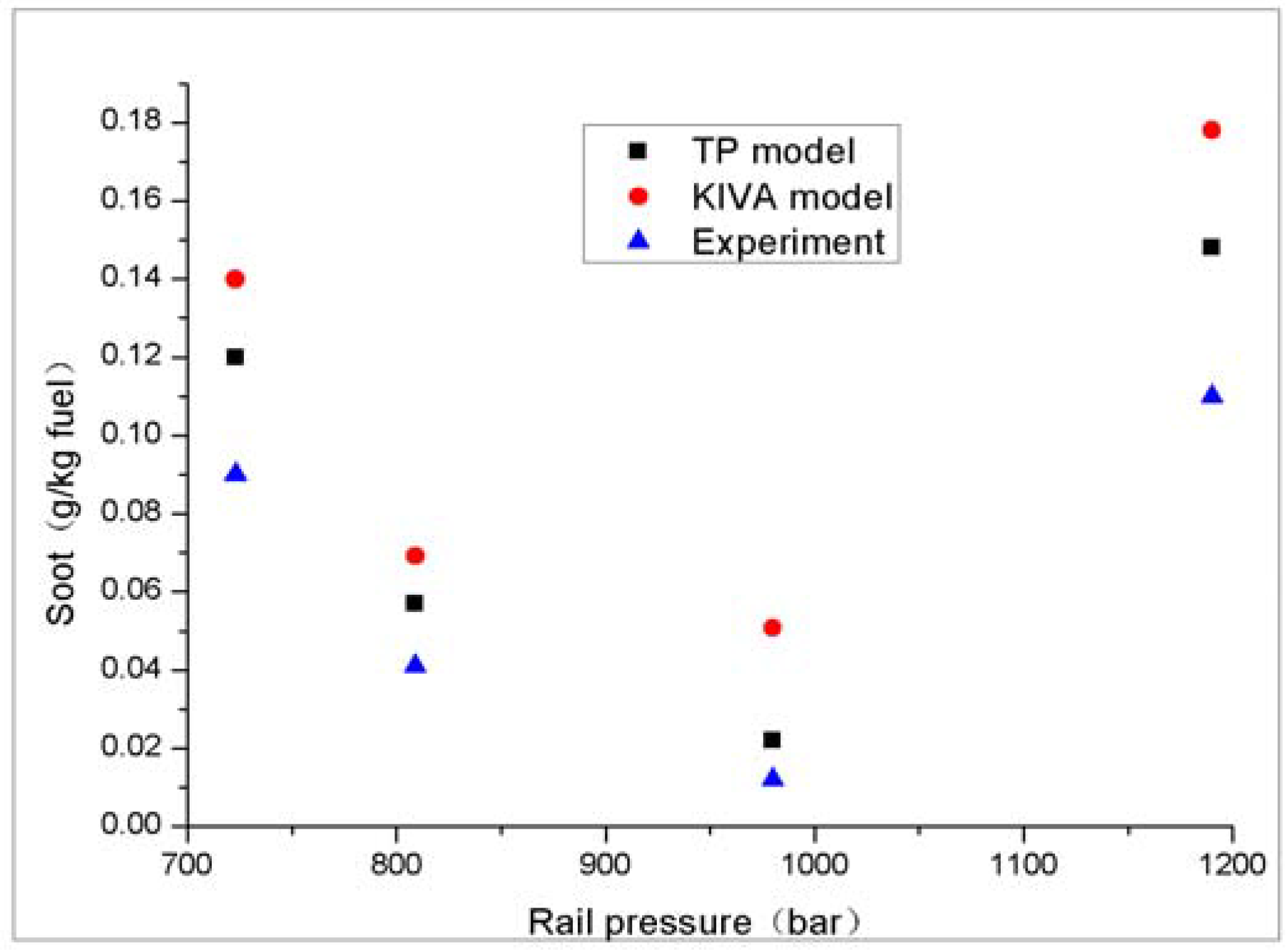
4.2.2. Summary of Investigated Load Conditions

Figure 9 summarizes the different parameter variations performed. It is seen that a variation of rail pressure leads to soot variation. When the rail pressure is 980 bar, soot source is the least (about 0.022 g/kg fuel). When the rail pressure is 1190 bar, soot source is the biggest (about 0.141 g/kg fuel). It means soot is related to capacity. When the capacity is increased, soot is increased. But it is not a proportional relationship. This is due to different working conditions caused by different injection times. For the initial injection, there is less fuel, and the amount of soot produced is smaller. For the second injection, the jet occurs at a high cylinder temperature. The chemical reaction is very quick and the ignition delay is very short. The sprayed fuel is quickly ignited and the generated soot is oxidized continuously, so the final generated soot is relatively small.
Figure 9. Summary of parameters variation study.
Energies 04 00894 g009
The original KIVA model and the improved TP model have the same tendency, but the improved model is closer to the experimental than the original model. In particular when the engine is at 2200 r/min (211 Nm) and 2700 r/min (195 Nm), the gaps are about 50%. This shows that the improved model is more realistic than the original model.

5. Conclusions

(1) Our improved combustion model can accurately predict cylinder pressure. Since the original KIVA-3V model reaction operates under the assumption that combustion is complete, it overestimates the heat release rate, in fact after all the fuel is oxidized, CO oxidation is still underway. Since the original KIVA-3V computational model of the activation energy has no real meaning, any calculation of cylinder pressure curves does not reflect the diesel ignition delay, while the use of this improved model can be used to calculate the ignition delay of diesel fuel.
(2) KIVA-3V calculates the heat release rate of the original model on the assumption that the ratio of combustion products CO and CO2 remains the same, but this does reflect the actual situation. The instantaneous heat release rate by the original model difference from the test value is 30%. The instantaneous heat release rate by the improved model is in good agreement with the experiment.
(3) The original KIVA-3V model did not calculate soot precursor—PAH, and did not consider the PAH growth and the initial particle density, so the soot formation by the original KIVA-3V model cannot reflect the actual situation. However, the modified soot model considers these factors, and the soot determination accuracy increases about 50%.

Acknowledgements

The authors thank Nobert Peters (RWTH-Aachen, Germany) for valuable discussions and Maggy McNorton (University of Glamorgan, UK) for checking English grammar and spelling. The study was sponsored by the Beijing Natural Science Foundation (3102011), China and Beijing University of Civil Engineering and Architecture Ph.D foundation (101001604) and Funding Project for Academic Human Resources Development in Institutions of Higher Learning under the Jurisdiction of Beijing Municipality (PHR (IHLB) 201008370, 201106125).

References

  1. United Nations Development Programme (UNDP). World Energy Assessment: Energy and the Challenge of Sustainability; UNDP: New York, NY, USA, 2008. [Google Scholar]
  2. Peters, N. Turbulent Combustion; Cambridge University Press: Cambridge, UK, 2004; pp. 1–5. [Google Scholar]
  3. Frenklach, M.; Wang, H. Soot Formation in Combustion-Mechanisms and Models; Springer Verlag: Berlin-Heidelberg, Germany, 2004; pp. 162–164. [Google Scholar]
  4. Mauss, F. Entwicklung eines Kinetischen Modells der Russbildung mit Schneller Polymerisation. Ph.D. Thesis, RWTH Aachen, Aachen, Germany, 1997. [Google Scholar]
  5. Balthasar, M.; Heyl, A.; Mauss, F. Flamelet modeling of soot formation in laminar ethyne/air diffusion flames. In Proceedings of the Twenty-Sixth Symposium (International) on Combustion, Naples, Italy; 1996; pp. 2396–2405. [Google Scholar]
  6. Barths, H. Simulation of Diesel Engine and Gas Turbine Combustion Using Multiple Flamelets with Detailed Chemistry. Ph.D. Thesis, RWTH-Aachen, Aachen, Germany, 2001. [Google Scholar]
  7. Liu, Y.; Pei, P. Analysis on ignition and extinction of n-heptane in homogeneous systems. Sci. China 2005, 48, 556–569. [Google Scholar] [CrossRef]
  8. Liu, Y. Analysis on three dimensional computational fluid dynamics software based on KIVA-3V code. In Proceedings of the 3rd International Conference on Computer Science & Education, Henan, China; 2008; pp. 259–263. [Google Scholar]
  9. Liu, Y. Optimization research for a high pressure common rail diesel engine based on simulation. Int. J. Automot. Technol. 2010, 11, 625–636. [Google Scholar] [CrossRef]
  10. Liu, Y. Mesh Generation and Dynamic Mesh Management for KIVA-3V. J. Beijing Inst. Technol. 2009, 17, 41–45. [Google Scholar]
  11. Amsden, A.A. KIVA-3V, Release 2, Improvements to KIVA-3V; Technical Report LA-13608-MS; Los Alamos National Laboratory: Los Alamos, NM, USA, 1999.
  12. Zimmer, L.; Tachibana, S. Laser induced plasma spectroscopy for local equivalence ratio measurements in an oscillating combustion environment. Proc. Combust. Inst. 2007, 31, 737–745. [Google Scholar] [CrossRef]
  13. Wang, Y.; Rutland, C.J. Direct numerical simulation of ignition in turbulent n-heptane liquid-fuel spray jets. Combust. Flame 2007, 149, 353–365. [Google Scholar] [CrossRef]
  14. Hergart, C.A. Modeling Combustion and Soot Emissions in a Small-Bore Direct-Injection Diesel Engine; Shaker Verlag: Aachen, Germany, 2001; pp. 10–22. [Google Scholar]
  15. Balthasar, M.; Frenklach, M. Detailed kinetic modeling of soot aggregate formation in laminar premixed flames. Combust. Flame 2005, 140, 130–145. [Google Scholar] [CrossRef]
  16. Netzell, K.; Lehtiniemi, H.; Mauss, F. Calculating the soot particle size distribution function in turbulent diffusion flames using a sectional method. Proc. Combust. Inst. 2007, 31, 667–674. [Google Scholar] [CrossRef]
  17. Morgan, N.; Kraft, M.; Balthasar, M.; Wong, D.; Frenklach, M.; Mitchell, P. Pablo Mitchell Numerical simulations of soot aggregation in premixed laminar flames. Proc. Combust. Inst. 2007, 31, 693–700. [Google Scholar] [CrossRef]
  18. Tao, F.; Golovitchev, V.I.; Chomiak, J. A phenomenological model for the prediction of soot formation in diesel spray combustion. Combust. Flame 2004, 136, 270–282. [Google Scholar] [CrossRef]
  19. Dec, J.E.; Coy, E.B. OH Radical Imaging in a D.I. Diesel Engine and the Structure of the Early Diffusion Flame. In Proceedings of the International Congress and Exposition of the SOCIETY of Automotive Engineers (SAE), Detroit, MI, USA, 26–29 February 1996.
  20. Dec, J.E.; Canaan, R.E. PLIF Imaging of NO Formation in a DI Diesel Engine. SAE Paper No. 980147. SAE Trans. 1998, 107, 176–204. [Google Scholar]
  21. Dec, J.E.; Kelly-Zion, P.L. The Effects of Injection Timing and Diluent Addition on Late-Combustion Soot Burnout in a DI Diesel Engine based on Simultaneous 2-D Imaging of OH and Soot. SAE Paper No. 2000-01-0238. SAE Trans. 2002, 109, 1–10. [Google Scholar]
  22. Bouvier, Y.; Mihesan, C.; Ziskind, M.; Therssen, E.; Focsa, C.; Pauwels, J.F.; Desgroux, P. Molecular species adsorbed on soot particles issued from low sooting methane and acetylene laminar flames: A laser-based experiment. Proc. Combust. Inst. 2007, 31, 841–849. [Google Scholar] [CrossRef]
  23. Marjamaki, M.; Keskenin, J.; Chen, D.R.; Pui, D.Y.H. Performance Evaluation of the Electrical Low Pressure Impactor (ELPI). J. Aerosol Sci. 2000, 31, 249–261. [Google Scholar] [CrossRef]
  24. Harris, S.J.; Maricq, M.M. Signature size distributions for diesel and gasoline engine exhaust particulate matter. J. Aerosol Sci. 2001, 32, 749–764. [Google Scholar] [CrossRef]
  25. Schneider, J.; Hock, N.; Weimer, S.; Borrmann, S. Nucleation Particles in Diesel Exhaust: Composition Inferred from in Situ Mass Spectrometric Analysis. Environ. Sci. Technol. 2005, 39, 6153–6161. [Google Scholar] [CrossRef] [PubMed]

