2.1. Energy Sources in Industrial Plants
Potential heat sources are all the streams of the process considered that must be cooled. The heat removed from these streams is first used, whenever possible, inside the process to heat other streams which undergo a phase change or whose temperature has to be increased. This heat transfer is obviously limited by the condition that the temperatures of the streams losing energy be greater than the temperatures of the streams to which the energy is transferred.
A powerful implementation of this fundamental principle in process engineering is the well known and widely applied pinch technology [
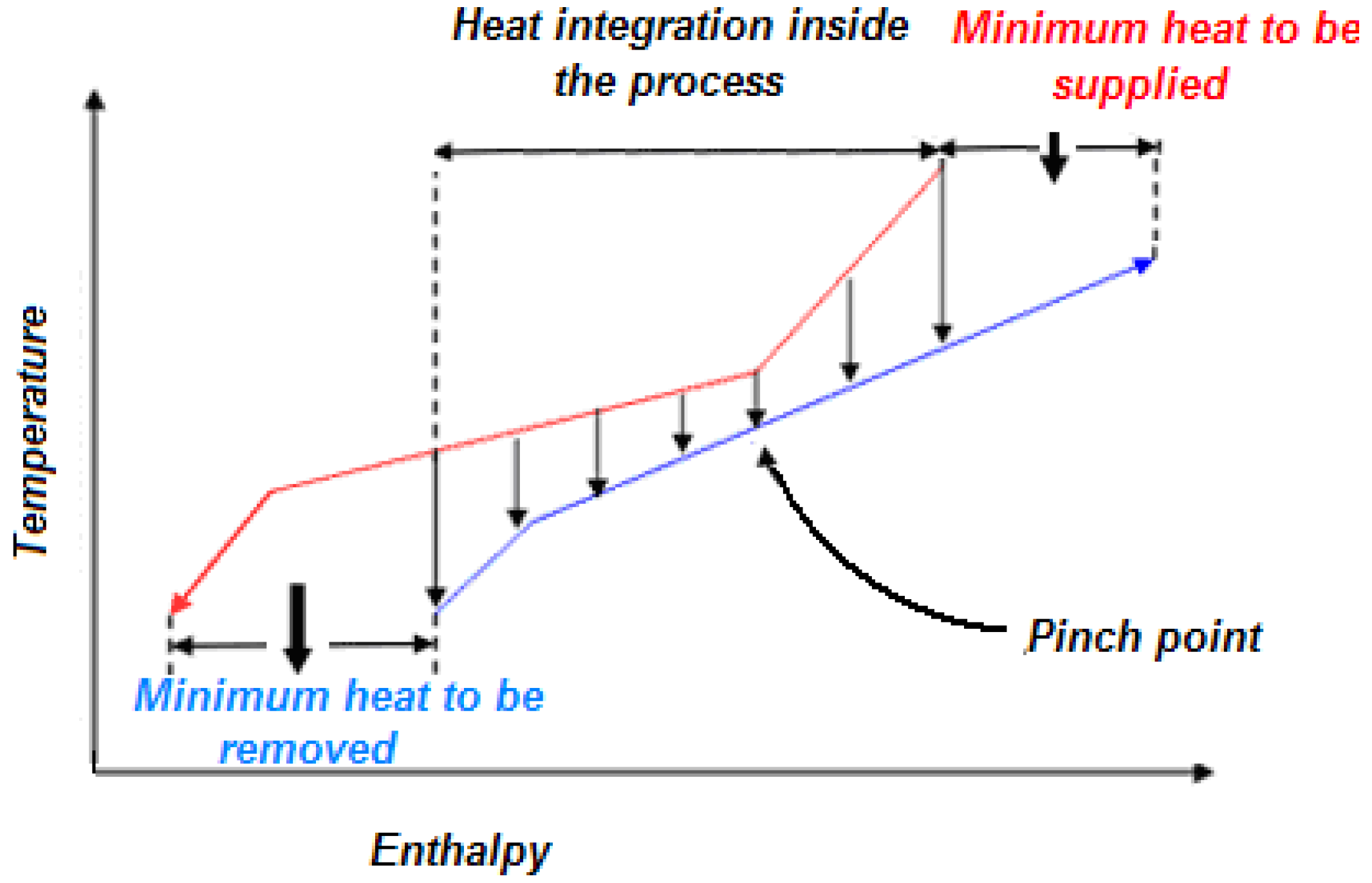
5]. The overall heat requirement is first calculated by plotting the thermal loads of the cold streams on a single graph (cold composite curve) in a temperature—enthalpy plane. If the specific heats remain constant in the temperature range of each stream, the resulting graph is a piecewise linear function with a slope equal to the inverse of the heat capacity of each stream or of a combination of them if temperature ranges overlap. Similarly, the thermal loads of the hot streams (
i.e., the streams that must be cooled) can be plotted in a similar graph to provide the hot composite curve. The optimal heat integration can be identified by letting the minimum temperature difference between the curves be equal to a suitably pre-determined ∆
T (
Figure 1).
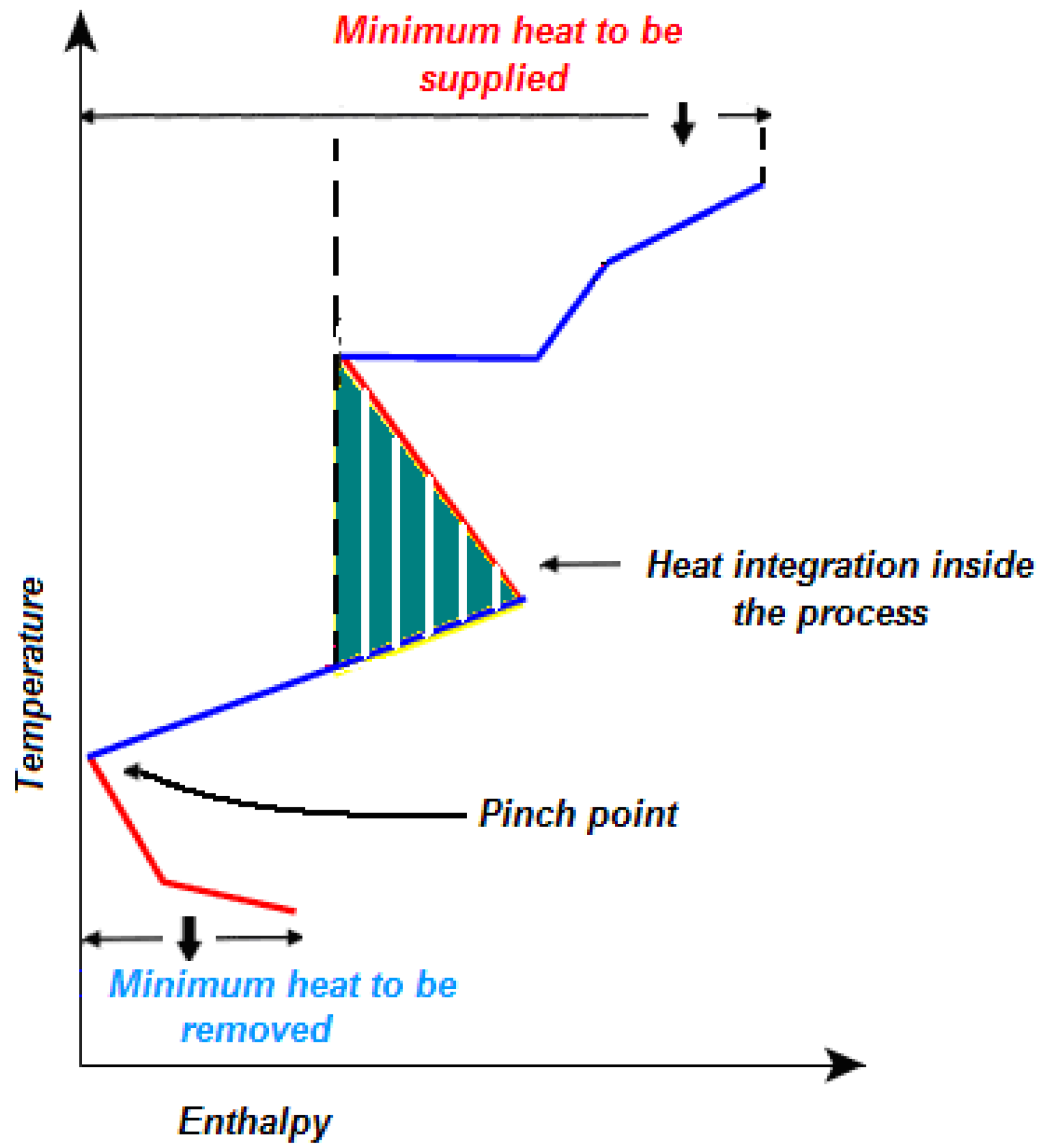
Figure 1.
Hot and cold composite curves of a generic process.
Figure 1.
Hot and cold composite curves of a generic process.
The corresponding temperature is called pinch temperature and the fundamental law of pinch technology is the requirement that no heat transfer take place across the pinch. Any such transfer would increase by the same amount both the overall heating and cooling requirement of the process. The grand composite curve can be constructed by plotting enthalpy differences between the composite curves at each temperature (
Figure 2).
The pinch point lies now on the temperature axis and temperature intervals in which hot streams lie above cold streams can be used for the heat integration of the process. The overall minimum thermal requirement and the minimum required amount of cooling water of the process can now be easily identified as the abscissas of the curve at maximum and minimum temperatures.
Figure 2.
Grand composite curve of a generic process.
Figure 2.
Grand composite curve of a generic process.
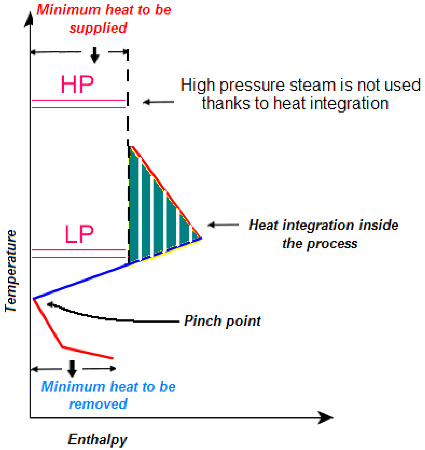
In addition to providing this information, the grand composite curve is a powerful tool that experienced process designers can take advantage of to optimally modify the configuration of the plant. For instance, in
Figure 3 optimal process integration makes it possible to use only low pressure steam, whereas the heat necessary at higher temperatures is provided by internal energy transfer.
Figure 3.
Process integration makes it possible to use low pressure steam only.
Figure 3.
Process integration makes it possible to use low pressure steam only.
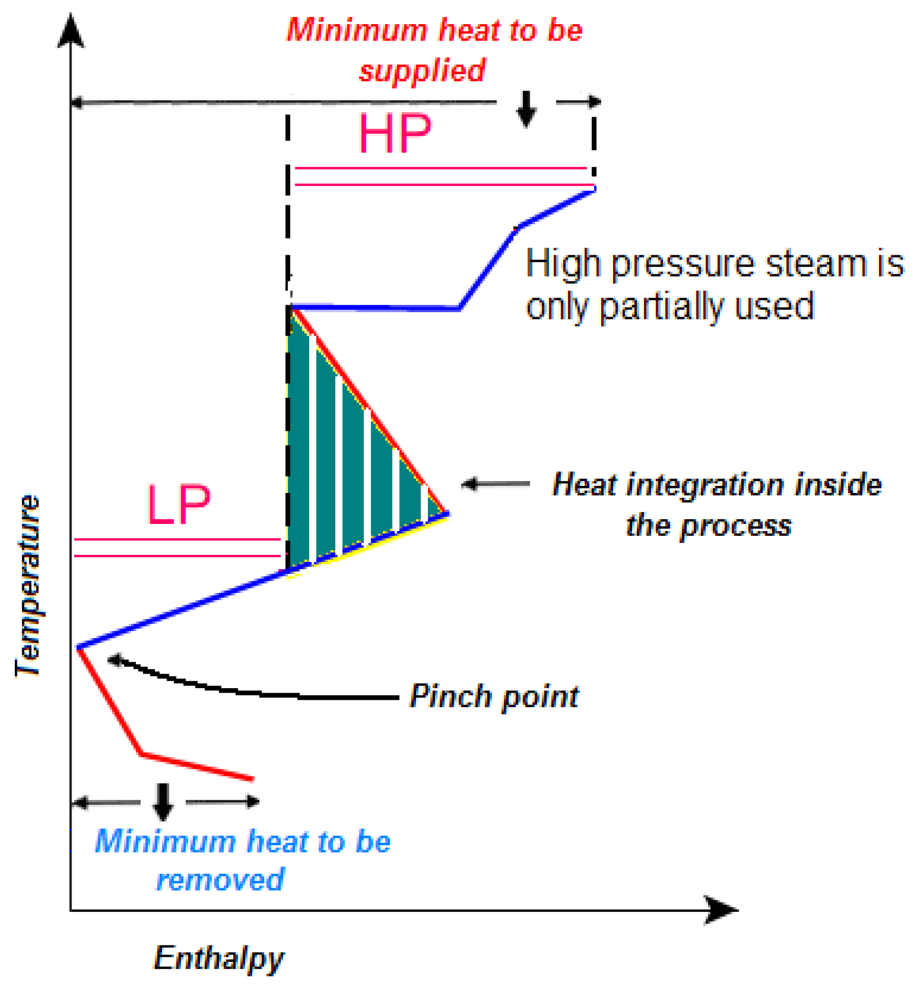
Similarly in
Figure 4 only part of the heat is provided by high pressure steam. By considering heat requirements at different temperatures the energy transfer is optimally split between the two steam lines.
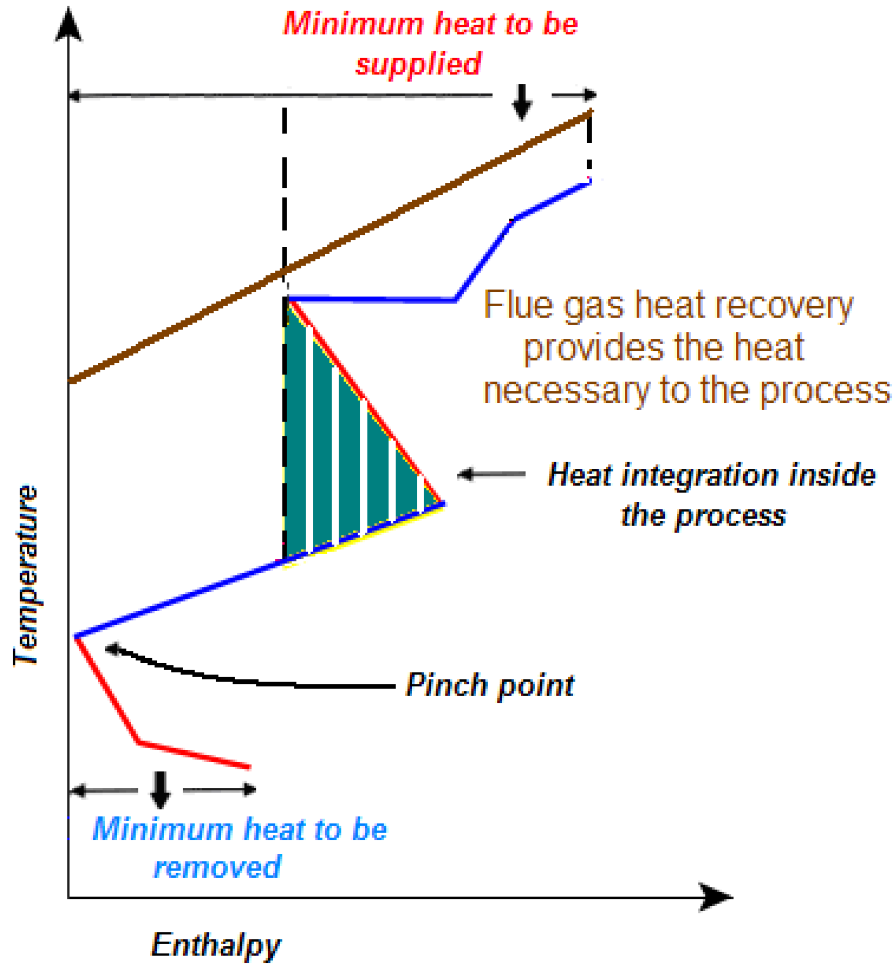
In
Figure 5 the use of internal energy transfer and the recovery of the enthalpy content of flue gases makes it possible to dispense with external energy sources. Indeed the flue gas temperature
vs. enthalpy curve (which is a straight line if the specific heat is approximately constant) lies entirely above the grand composite curve of the process and consequently it can supply all the necessary amount of heat.
Figure 4.
Reduced use of high pressure steam.
Figure 4.
Reduced use of high pressure steam.
Figure 5.
Recovery of flue gas enthalpy content.
Figure 5.
Recovery of flue gas enthalpy content.
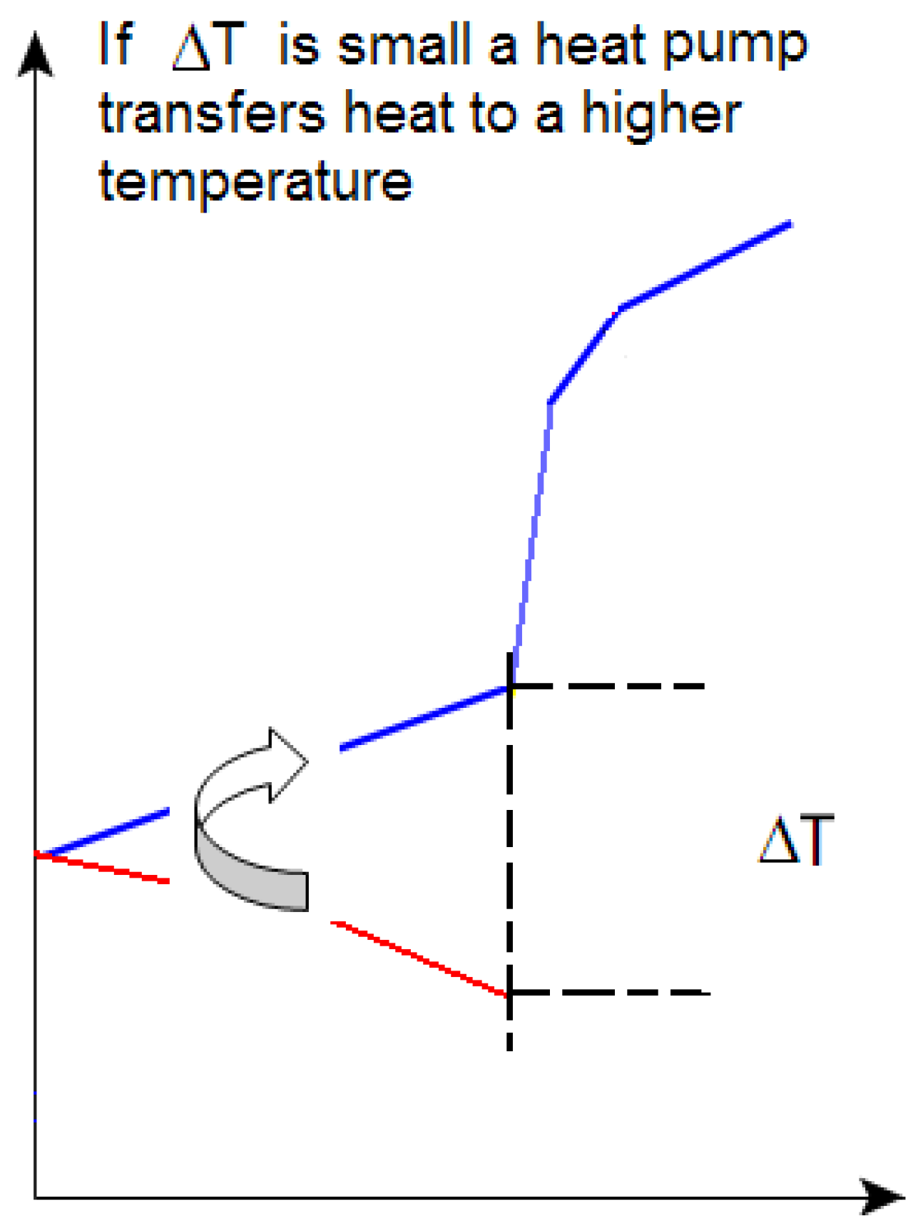
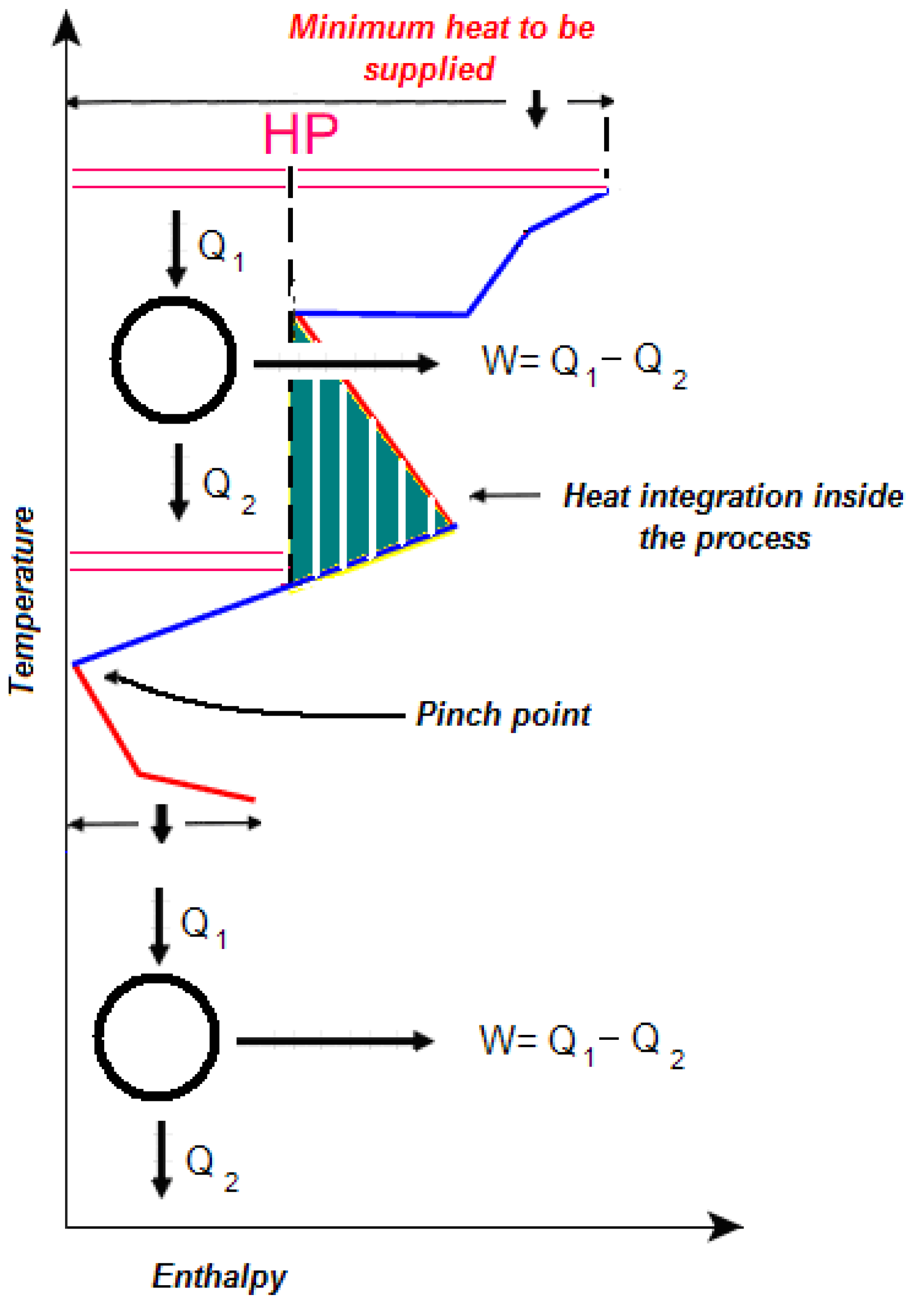
Sometimes external work may be a convenient way to raise the temperature at which heat is available. This is often the case when large amounts of heat are available just below the pinch temperature and corresponding amounts of energy are required at temperatures slightly superior to the pinch temperature (
Figure 6). In these cases the cost of using the work of heat pumps can be less (and sometimes much less) than the cost of the amount of heat saved. Obviously the use of available energy inside the process through heat integration has a higher priority than exporting energy outside of it.
Thus, the identification of potential heat sources in the design phase or in a retrofitting process should not consider the energy that might be conveniently used in a process integration analysis.
Similarly, total site integration (i.e., energy integration between different processes located at the same industrial site) can be considered a straightforward extension of the heat integration in a single process. Indeed, with respect to district heating/cooling it has the obvious advantage of a limited infrastructural effort.
Figure 6.
Use of a heat pump to exploit heat available below the pinch.
Figure 6.
Use of a heat pump to exploit heat available below the pinch.
Once both process and site heat integration has been carried out, the amount of energy available “across the fence” can easily be determined by simple inspection.
Below the pinch this can be expressed typically in the form:
where
is the power available in the temperature range:
and
cpk the average specific heat of the flowrates
Fk.
These constraints apply to all the temperature intervals N, where an energy export is available. Above the pinch the amount of energy available that can be transferred depends on how heat is supplied to the process. The excess heat can be recovered either generating shaft work in a turbine or exchanging heat with external fluids.
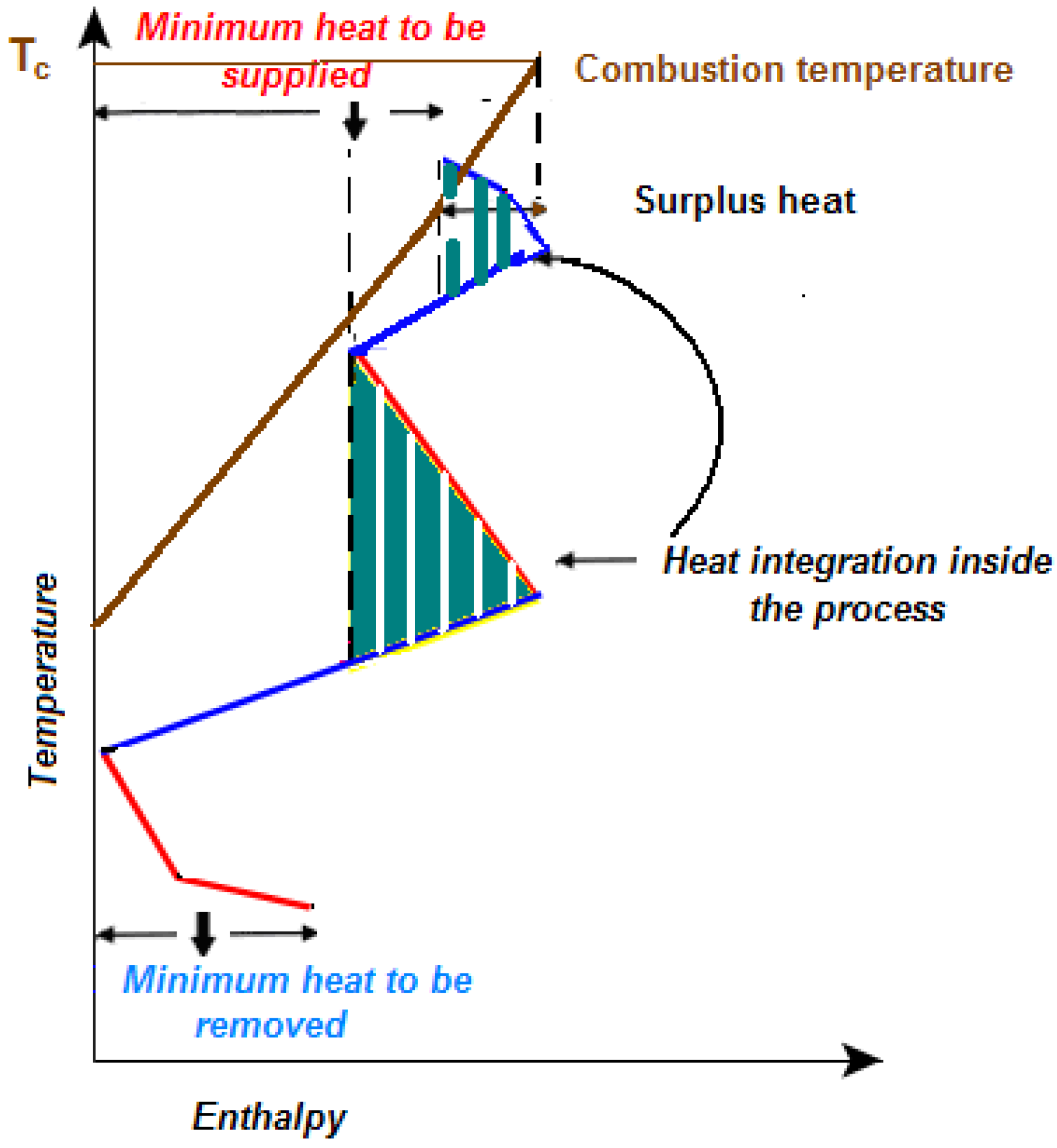
Thus, for instance, in
Figure 7 the amount of energy available when heat is supplied using the flue gases resulting from fuel combustion is shown. In this case part of the energy required by the process can be recovered through heat integration inside the process and consequently the flue gas can provide an amount of surplus heat from the combustion temperature to the temperature where energy transfer to the process is required.
Figure 7.
Determination of available heat when heat is supplied from fuel combustion.
Figure 7.
Determination of available heat when heat is supplied from fuel combustion.
2.2. Energy Transfer Options
2.2.1. Electrical Power
In industrial processes cogeneration (or combined heat and power generation, CHP) means production of electrical power by gas turbines (using flue gas resulting from fuel combustion,
Figure 7) or by steam turbines operating in a Rankine cycle using the available surplus heat. This is the main difference with large power stations where heat is a byproduct of power generation and gas turbines or reciprocating engines are normally used.
The key information provided by the pinch analysis is that the temperatures over which the Rankine cycle operates should not include the pinch point. Thus, the first possibility is provided by a Rankine cycle operating between two temperatures above the pinch temperature. This situation can arise when high pressure steam has to heat up a cold stream over a wide temperature range. As shown in
Figure 8 part of the high pressure steam can be fed to a turbine whose exhaust steam temperature is still high enough to provide the necessary heat to the lower temperature part of the stream.
Whenever the pinch temperature is high enough (as is the case for instance in the ammonia production process), a CHP system can be designed for cooling the hot streams without the necessity of using a coolant, which adds to the profitability of the process. Again a steam-operated Rankine engine is used to this purpose. The steam generated by the heat transferred from the process is the working fluid that powers the steam turbine.
If an Organic Rankine Cycle (ORC) is used, it is possible to recover heat from low temperature sources, thanks to the use of an organic fluid, which has a boiling point, at which the liquid-vapor phase change takes place, lower than the traditional water-steam system. This greatly increases the number of processes to which it can be applied.
Figure 8.
Cogeneration above and below the pinch.
Figure 8.
Cogeneration above and below the pinch.
Thus, the temperature range over which the combined heat and power generation is possible frequently overlaps the range traditionally used for district heating/cooling. Hence the necessity of developing an optimisation algorithm for the most convenient distribution of waste heat from processes between the two options.
2.2.2. District Heating and Cooling
Water is the most frequently used medium to distribute heat collected from various sources to dwellings and offices through heat substations, although steam is sometimes used [
6]. As anticipated before, an intermediate storage greatly adds to the profitability of the system.
The size of district heating systems varies from covering large urban areas to small villages and even to a limited number of households. According to the size of the system there can be, in addition to the primary radial or ring-shaped piping networks, secondary and tertiary circuits with decreasing pipe diameter, whose shape and size is adapted to the urban structure served by the system.
In addition to the recovery of surplus heat which otherwise would be released to the environment, district heating reduces the investment costs for domestic or commercial heating equipment. However, this cost reduction is more than offset by the capital costs for the construction of district heating networks. Therefore areas with a low population density or small building compounds are generally not suitable for district heating, as investment costs per household would be considerably high.
The energy generated or stored can be used also for cooling purposes,
i.e., for providing chilled water to households and commercial space. The change from a district heating to a district heating/cooling system may guarantee the affordability and financial sustainability of a large scale project, in that both storage capacity and electrical power are considerably reduced [
7]. Indeed the seasonal heat storage is limited to the autumn months for the heating period and to spring for the cooling time, as opposite to a spring/summer/autumn storage time in the purely heating scheme. Obviously the storage capacity is reduced correspondingly.
Similarly electricity consumption is greatly reduced if heat driven refrigerators (such as absorption refrigerators, [
8]) are used, instead of the traditional compressor refrigerators. Up to 90% electricity consumption reduction can be achieved in this case.
2.3. The Underground Thermal Energy Storage
The installation of intermediate heat storage on a seasonal basis greatly adds to the overall profitability of a district heating system, as the energy produced in periods of limited consumption is not dispersed to the environment. Additionally, it can even out variable energy demands. However, it requires larger volumes than storages used for intermittent renewable sources based on a day/night or windy/calm weather cycle. Obviously, larger containers give rise to considerable investment costs, which play a key role in the feasibility study and cost/benefit analysis of a district heating/cooling project.
Considerable savings can be attained by storing the available heat using a natural medium. With respect to the construction of large steel or concrete reservoirs (above or partially below ground), underground thermal energy storage (frequently referred to with the acronym UTES) can reduce the payback time of capital costs to approximately 5–10 years [
9].
Indeed large quantities of heat can be stored in underground geological structures such as aquifers (ATES), natural or artificial caverns and disused mines (CTES) or drilling borehole thermal energy storage structures (BTES).
Occasionally, the two technologies are combined: a high temperature storage vessel embedded in an underground structure, which is kept at a lower temperature and from which heat is extracted using heat pumps. This makes it possible to recapture some of the heat released by the central vessel to the external environment.
Indeed heat losses to the environment depend heavily on temperature, size and nature of the storage system considered. This has to be taken into account in the general optimisation procedure by considering different options separately. Alternatively, a preliminary optimisation of suitably identified subsystems can be carried out with respect to a limited number of parameters, which are then kept fixed at their optimum values in the general optimisation procedure.
Thus for instance heat-driven cooling can be either dispersed or decentralised [
10] according to whether the chilled water used for cooling is generated by small chillers located in each user’s building (thus dispensing with chilled water distribution) or through small cooling substations based on absorption technology (thus reducing chilled water distribution costs and eliminating the necessity of installing chillers in each building). Once the better solution for the particular case considered has been identified, it can be used in the general optimisation procedure.
2.4. Model for the Identification of the Optimal Configuration
The overall optimal configuration can be evaluated if a suitable objective function is defined subject to the constraints. Typically the objective function depends on the revenue from energy transferred outside the plant and on both capital and operating costs related to the energy transfer process.
Each heat source i (i = 1,…,N) not used inside the process can be used either for power generation or for district heating/cooling. The number of heat sources is equal to the number of temperature ranges over which heat is available. For large temperature ranges more than one heat source can be considered.
The annual revenue for each of them is given by b1i·(εi·c − m1i) + b2i·(Hi·d − m2i) where bi is the binary value {0,1}, εi and Hi the yearly amounts of power generated or of heat transferred to a district heating system in one year and c and d their prices. m1i and m2i are operating and maintenance costs of the equipment operating in the interval i. The product b1i·b2i must obviously be equal to zero (the available energy is used for electrical work, for heat transfer or released to the environment, the latter condition being given by the condition that both b1i and b2i are zero.
The capital costs are the turbine/generator equipment for the cogeneration and heat exchangers and volume and nature of the underground storage for the district heating. The annual fixed charges f can be computed by dividing the capital costs by the total years of useful life (supposing salvage values equal to zero).
Thus a reasonable objective function is:
subject to:
which is to be minimised subject to the mass and heat balances that must be taken into account in the overall system. Both
and
Hi are equal to
to a factor of proportionality for changing kW to kWh/year. This is not just a conversion factor, as it takes into account the number of operating hours in a year.
Obviously additional factors could be introduced into the objective function. Typically they might include terms related to robustness (with a view to minimising the number of faults of the system) and to resilience (so that the overall system can adapt to changes in exogenous variables, while remaining technically stable and financially feasible).
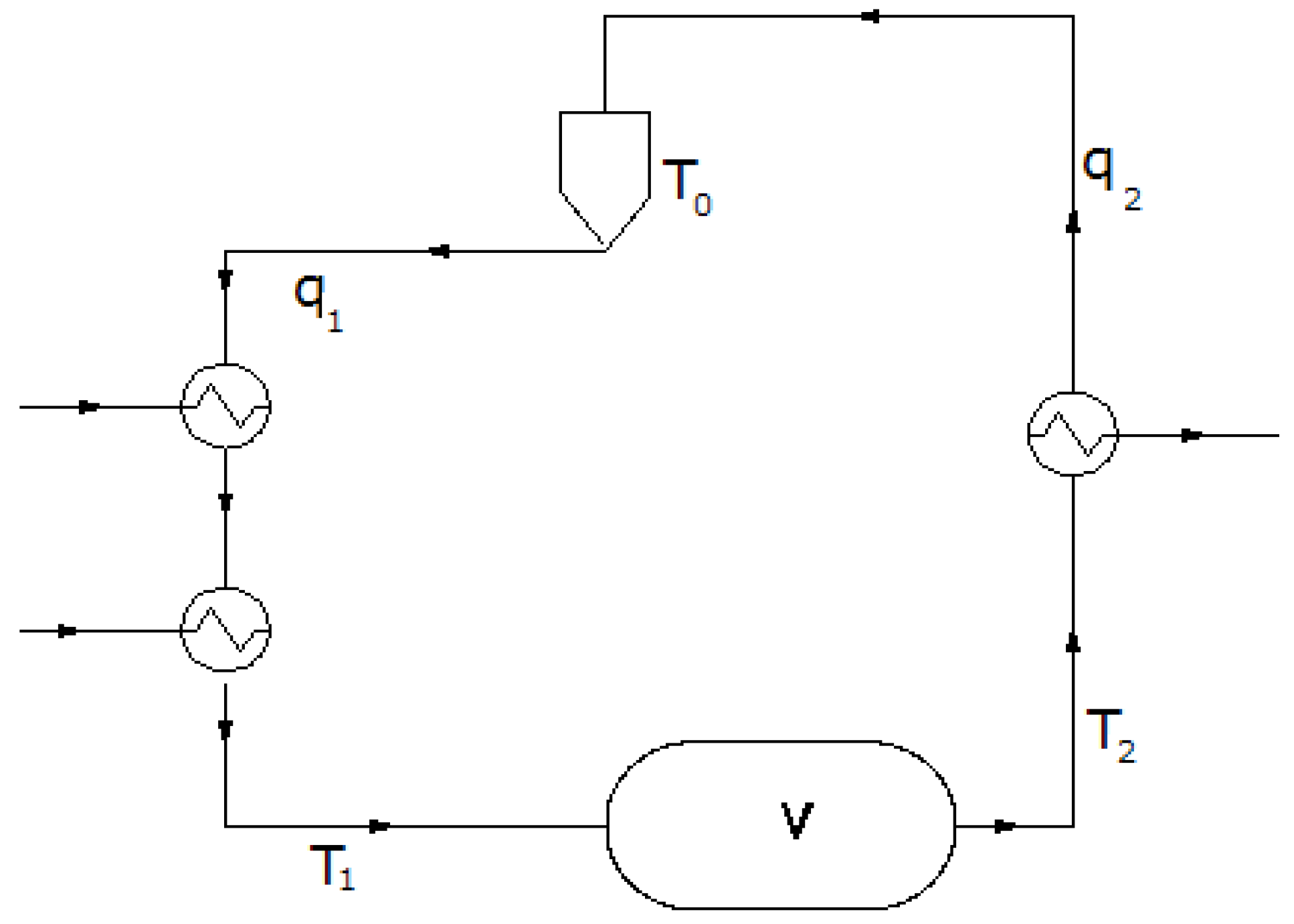
Additional equality constraints are provided by the energy and mass conservation law. The energy transfer balance between the process and the district heating system is given by (see
Figure 9):
Figure 9.
Conceptual scheme of a district heating network with an intermediate storage.
Figure 9.
Conceptual scheme of a district heating network with an intermediate storage.
Similarly the energy transfer between the district heating system and the final user is given by:
where
is the heat demand from final users (which has to be estimated on basis of historical demand values) and
Tu(
t) is the temperature of the underground storage.
The mass and energy balances in the underground storage can be expressed as:
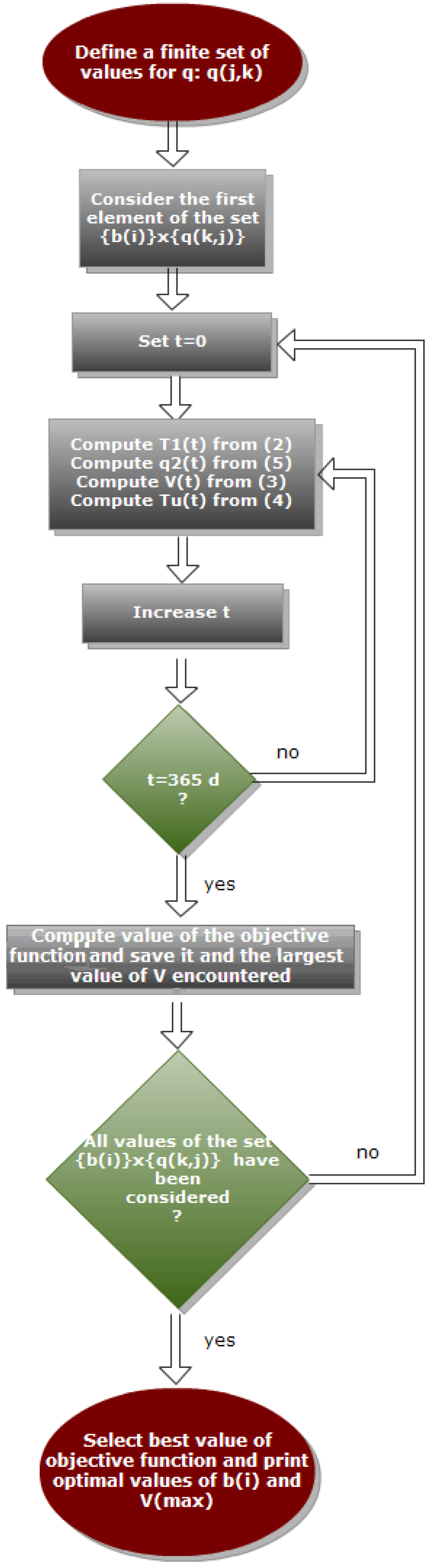
The minimisation has to be carried out with respect to the set over the span of one year. For every value of , T1(t) can be calculated from Equation (2), q2(t) from Equation (3), V(t) from the integration of Equation (4) and Tu(t) from the integration of Equation (5).
Once the minimisation has been carried out, the optimal values of and the maximum value of V(t) found in the time range considered provide all the information necessary to carry out the design of the cogeneration equipment and of the district heating/cooling system, including the volume of the underground thermal energy storage.
Obviously in case the minimum value of Φ should turn out to be positive, the investment costs would exceed the financial benefits: the project would not be profitable and would not be implemented.
2.5. Numerical Algorithm for the Solution of the Optimisation Problem
The function
q1(
t) can be parametrised in terms of a finite number of parameters, the simplest approximation being a piecewise constant function:
Figure 10.
Flow chart of the optimisation algorithm.
Figure 10.
Flow chart of the optimisation algorithm.
The number of intervals can be set equal to the number of periods in the year during which is approximately constant. Thus the space of independent variables is changed into the finite dimensional space .
The optimization with respect to is carried out by enumeration, i.e., all the combinations are considered and the minimisation is carried out with respect to the set . The best combination is then considered for the determination of .
While the minimisation of (1) with respect to the set with fixed values of can in principle be carried out using rigorous gradient methods, considering GP equally spaced values of over a convenient grid (i.e., ) is a reasonable approximation which greatly simplifies the optimisation task. Additionally convergence to a sub-optimal local minimum (which might occur if a gradient method is used) can be avoided.
In other words, the solution of Equations (2–5) is carried out for each element of the (2
N ×
TP ×
GP)
-dimensional set
and the objective function is computed for each solution. Again the combination of values that provide the best value of the objective function is the sought after solution of the optimisation problem. The flow-chart of the minimisation procedure is shown in
Figure 10. For the sake of illustration simplicity energy losses have not been considered. However, they can easily be introduced by suitably modifying the energy balances (2), (3), (5). As mentioned in
Section 3, different types of heat storage can have different expressions for leaks and losses. In this case too, the procedure has to be repeated for each scenario and the corresponding values of the objective function should be examined for comparison. Obviously this increases further the enumeration effort. However, due to the computational efficiency with which the system of Equations (2–5) can be solved, the overall optimum can be located with an affordable computational time.

