Article

Map-Based Repowering and Reorganization of a Wind Resource Area to Minimize Burrowing Owl and Other Bird Fatalities

1
Research Ecologist, 3108 Finch Street, Davis, CA 95616, USA
2
Gis Specialist, Neher Consulting, 7241 34th Street, North Highlands, CA 95660, USA
3
East Bay Regional Park District, 2950 Peralta Oaks Court, Oakland, CA 94605-0381, USA
*
Author to whom correspondence should be addressed.
Energies 2009, 2(4), 915-943; https://doi.org/10.3390/en20400915
Submission received: 26 August 2009 / Accepted: 19 October 2009 / Published: 23 October 2009
(This article belongs to the Special Issue Wind Energy)

Abstract

:
Wind turbines in the Altamont Pass Wind Resource Area (Alameda/Contra Costa Counties, California, USA) generate about 730 GWh of electricity annually, but have been killing thousands of birds each year, including >2,000 raptors and hundreds of burrowing owls. We have developed collision hazard maps and hazard ratings of wind turbines to guide relocation of existing wind turbines and careful repowering to modern turbines to reduce burrowing owl fatalities principally, and other birds secondarily. Burrowing owls selected burrow sites lower on slopes and on smaller, shallower slopes than represented by the average 10 × 10 m2 grid cell among 187,908 grid cells sampled from 2,281,169 grid cells comprising a digital elevation model (DEM) of the study area. Fuzzy logic and discriminant function analysis produced likelihood surfaces encompassing most burrowing owl burrows within a fraction of the study area, and the former corresponded with burrowing owl fatalities and the latter with other raptor fatalities. Our ratings of wind turbine hazard were more predictive of burrowing owl fatalities, but would be more difficult to implement. Careful repowering to modern wind turbines would most reduce fatalities of burrowing owls and other birds while adding about 1,000 GWh annually toward California’s 33% Renewable Portfolio Standard.

1. Introduction

Policy-makers have hoped that wind energy generation in the Altamont Pass Wind Resource Area (APWRA) will contribute to meeting both California’s growing energy demand and its recent mandates on renewable energy use. California’s Governor Arnold Schwarzenegger issued Executive Order S-14-08 (17 Nov 2008), requiring that 33% of the energy delivered to California consumers shall come from renewable sources by the year 2020. Executive Order S-14-08 was termed the 33% Renewable Portfolio Standard (33% RPS). Given the energy used in 2006 and assuming the California Energy Commission’s projected 1.2% annual growth in consumption, the renewable resource gap is 80,690 GWh. For perspective, the APWRA’s installed capacity of 580 MW generated 730 GWh in 2006, or 0.9% of the renewable resource gap, but it has been killing thousands of birds per year since its development in the 1980s [1,2].
The locations for APWRA wind turbines were selected without considering patterns of bird flights, perching or nest locations, all of which influence collision risks. Most wind turbines were mounted on short towers, which positioned the rotor planes at heights above ground that are often used specifically for foraging by golden eagle, red-tailed hawk, American kestrel, and burrowing owl, and these species have subsequently been killed at high rates in the APWRA. Of particular concern are burrowing owl fatalities, estimated at 99 to 380 [3] and 440 per year in 1998–2003 [4], and 737–1,488 per year in 2005–2007 [2]. Whereas the more recent estimate might be inflated due to a possible bias in the scavenger removal adjustment [2], all of these fatality rates and those of other species [2] indicate the APWRA has been in excessive violation of the international Migratory Bird Treaty Act, Federal Bald and Golden Eagle Protection Act, and California Fish and Game Code 3503.5 (Birds of Prey). Burrowing owls have been declining in California [5,6,7], and are listed as a second-priority species of special concern in California [8], therefore, there is urgent need to sharply reduce burrowing owl fatalities caused by the APWRA’s wind turbines.
After several years of research of bird behaviors and fatalities in the APWRA, it was concluded that careful repowering would reduce fatalities more so than the 16 mitigation measures formulated for continued operation of the old-generation turbines [9]. Careful repowering would replace old-generation wind turbines with modern turbines on taller towers and located where collision risk is minimized. Two small repowering projects were installed since the earlier recommendation for repowering. These were the 20.5 MW Diablo Winds Energy Project and the 38 MW Buena Vista Wind Energy Project, which began operations in 2004 and 2007, respectively. Compared to old-generation wind turbines in the APWRA, raptor fatalities per MW per year were 54% lower at Diablo Winds [2] and 91% lower at Buena Vista [10]. Since repowering, burrowing owl fatalities have not been found at Buena Vista and declined 24% at Diablo Winds compared to concurrently operating old-generation wind turbines [2].
Given that repowering of the APWRA is moving forward slowly and in piecemeal fashion a burrowing owl collision hazard map could help reduce burrowing owl fatalities immediately by showing which old-generation wind turbines pose the greatest risk to this species and where these turbines might be relocated to reduce collision risk [11,12]. A collision hazard map could reduce burrowing owl fatalities more substantially over the longer term by guiding where modern wind turbines are sited as repowering expands. One caveat to this hazard mapping approach is inter-specific variation in avian behavior in response to environmental and wind turbine attributes such that a least-hazards map developed for burrowing owls could potentially increase the collision risk for other species.
Earlier research established a positive relationship between burrowing owl fatalities and the number of burrowing owl burrows within 55 m of wind turbines [13], and a model based on a set of turbine and landscape attributes correctly predicted 71% of the burrowing owl fatalities documented in 1998–2003 [3]. Thus it is reasonable to assume that predicted burrowing owl burrow locations would correspond with wind turbine collision hazard, and this information could be used to develop a burrowing owl collision hazard map. In the APWRA, burrowing owls usually commandeer burrows from burrow systems constructed by California ground squirrels (Spermophilus beecheyi), so to develop a map predicting burrowing owl burrow locations we needed to know which portions of the landscape are selected by ground squirrels and which of this portion selected by ground squirrels is also selected by burrowing owls.
The goal of our study was to develop a predictive model of burrowing owl burrow locations in the APWRA to be used as a map-based indicator of collision hazards for relocating existing, old-generation turbines and guiding new-generation turbine siting in repowering. Our objectives were to: (1) develop predictive models of burrowing owl burrow locations; (2) validate the models by relating predicted burrowing owl burrow locations to documented locations, both within the spatial areas used to develop the predictive model and within an area that did not contribute to model development, i.e., Vasco Caves Regional Preserve, (3) validate the usefulness of the models by comparing burrowing owl fatality rates between turbines within areas predicted to be occupied by burrowing owls and turbines outside these areas, (4) compare the usefulness between a landscape-based hazard model and a wind turbine rating system based on environmental and wind turbine attributes associated with individual wind turbines, and (5) compare the tradeoffs of impacts of a burrowing owl management focus on other bird species, especially other raptors that often collide with the APWRA wind turbines.

2. Study Area

The APWRA encompassed about 16,450 ha of mostly non-native annual grassland in eastern Alameda and southeastern Contra Costa Counties in central California. The study area ranged 78 to 470 m above MSL, composed of hills, ridges and valleys, including ephemeral streams, stock ponds, seasonal ponds, and marshes. Most ridges were oriented northwest-southeast, increasing in size westward. Landowners grazed livestock and leased land to wind companies.
The APWRA included 580 MW of wind turbines of various models (Figure 1) during the 1998–2003 study [2], numbering about 5,400 in 1998 and 5,301 in 2003. In 2005, the Diablo Winds Project replaced 105 150-kW and 25 250-kW Flowind vertical axis wind turbines with 38 Vestas 660-kW turbines (Figure 2). By the end of 2006 the Buena Vista Wind Energy project replaced 170 Windmaster, Nordtank, and Danwin turbines with 38 1-MW Mitsubishi turbines (Figure 2).
Data for model development were gathered at multiple locations around wind turbines throughout the central, eastern, and southern portions of the APWRA. Data for model validation were also gathered from Vasco Caves Regional Preserve near the northern boundary of the APWRA, including 52 330-kW Howden turbines and 20 65-kW Nordtank turbines (Photos A and F in Figure 1). Vasco Caves Regional Preserve was managed by East Bay Regional Park District, and consists of five relatively large, steep hills. Wind turbines occupied only one of the large hills and a plateau on the northern aspect of the Preserve [14].

3. Methods

3.1. Estimating Fatality Rates

Fatality search effort varied in frequency and number of turbines searched throughout the study period 1998–2003 [4]. During fatality searches biologists searched for bird carcasses within 50 m of each wind turbine, walking parallel routes at about 8–16 m intervals along rows of turbines. From March 1998 through September 2002, groups of turbines were added to the search rotation as access was granted and ultimately a total of 1,526 wind turbines arranged in 182 rows were searched at various intervals (mean = 53 days). From November 2002 to May 2003 another 2,548 turbines arranged in 380 rows were searched twice at intervals of 90+ days. Carcasses found in 1998–2003 were used for developing predictive models. Carcasses found during another monitoring period, from March 2005 through March 2007 [2], were used for model validation. Searches for these carcasses were performed with an average interval of 41 days at 2,650 wind turbines in stratified random plots, using comparable field methods to the earlier fatality monitoring program.
All carcasses or body parts found were examined to assign species, age, sex, and probable cause of death. Cause of death was determined by evidence of injuries, when available, such as burn marks or singed feathers typical of electrocution, and cut or twisted torsos, dismemberment and other forms of blunt force trauma typical of collisions with wind turbine blades. Unless assigned another cause of death, carcasses were assumed to have been killed by a wind turbine if found within 125 m of a wind turbine. Carcasses were used in fatality rate estimation if the estimated time since death was ≤90 days, because we did not want to include fatalities caused prior to the study period. The number of days since death was estimated after assessing carcass condition (e.g., fresh, weathered, dry, bleached bones) and decomposition level (e.g., flesh color, presence of maggots, odor).
Figure 1. 
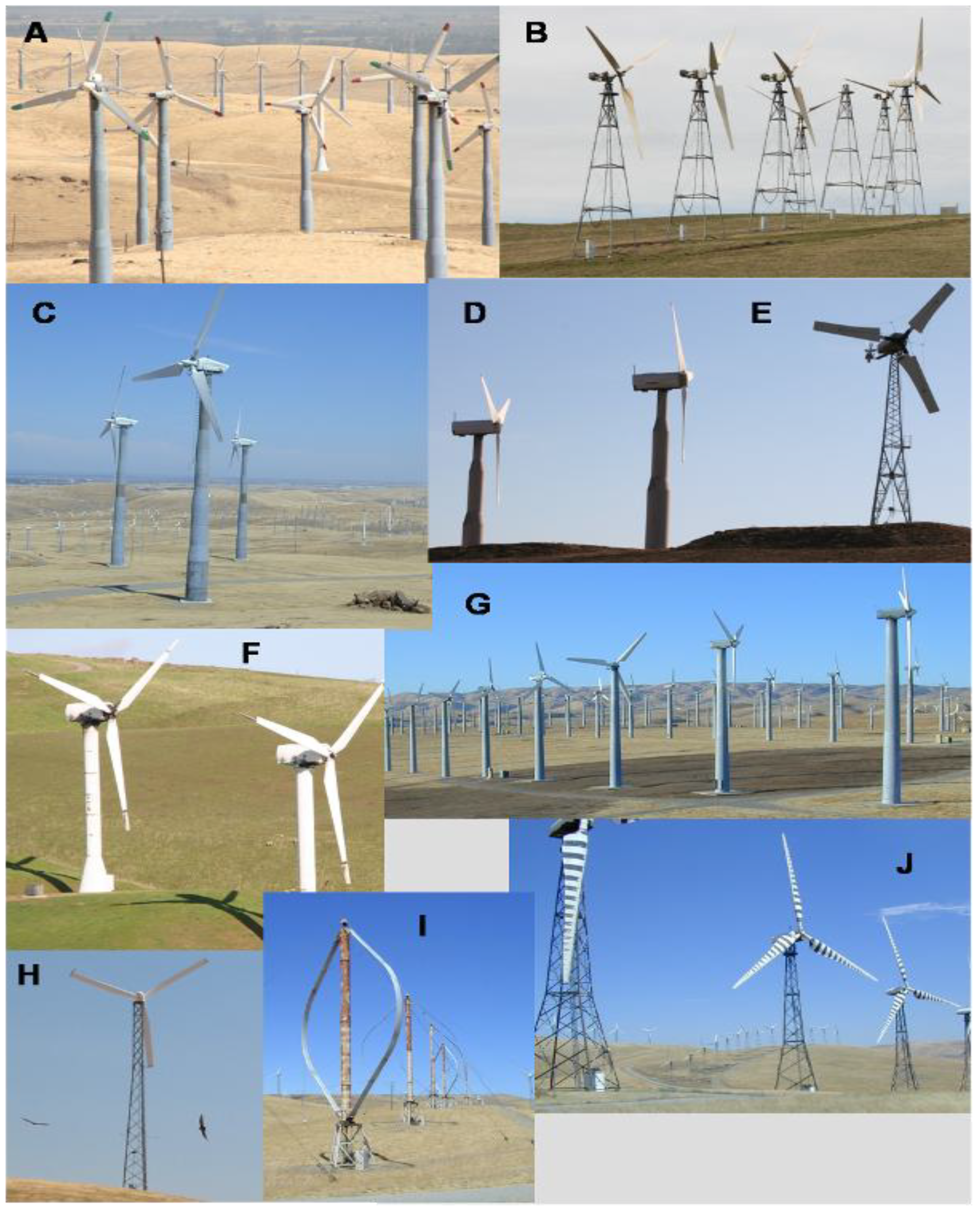
Some of the various old-generation wind turbine models in the APWRA during 1998-2007, including Nordtank 65-kW (A), KCS56 100-kW (B), Bonus 150-kW (C), Polenko 100-kW (D), Windmatic 65-kW (E), Howden 330-kW (F), Micon 65-kW (G), Enertech 40-kW (H), Flowind 150-kW (I), and KVS-33 400-kW (J). These photos are not to scale.
Energies 02 00915 g001
Figure 2. 
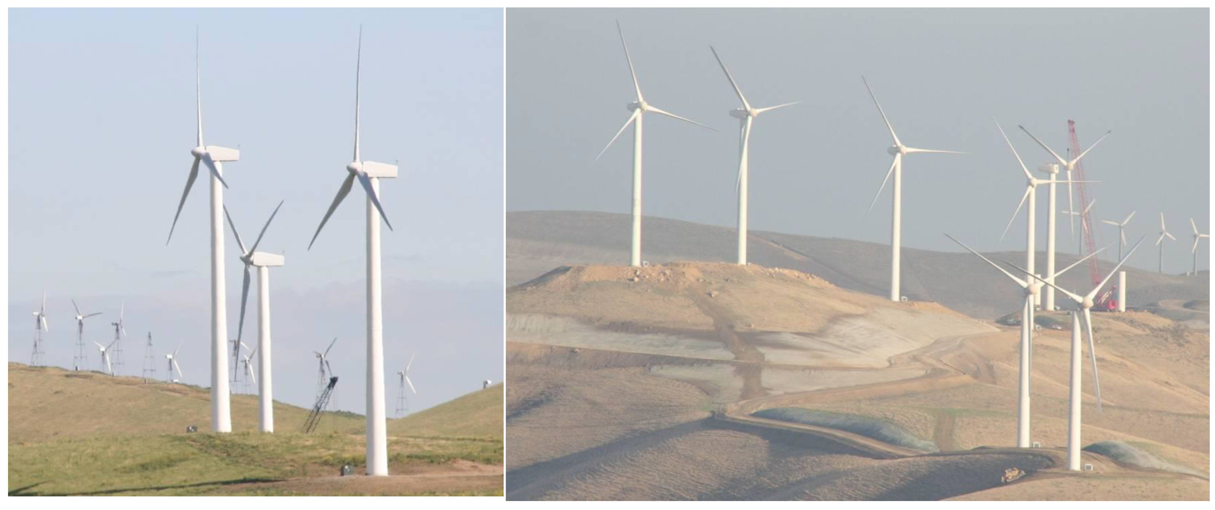
Vestas 660-kW turbines in Diablo Winds Energy Project, which replaced Flowind vertical axis turbines (left photo), and Mitsubishi 1-MW turbines in Buena Vista Wind Energy project that replaced Windmaster, Nordtank, and Danwin turbines (right photo).
Energies 02 00915 g002
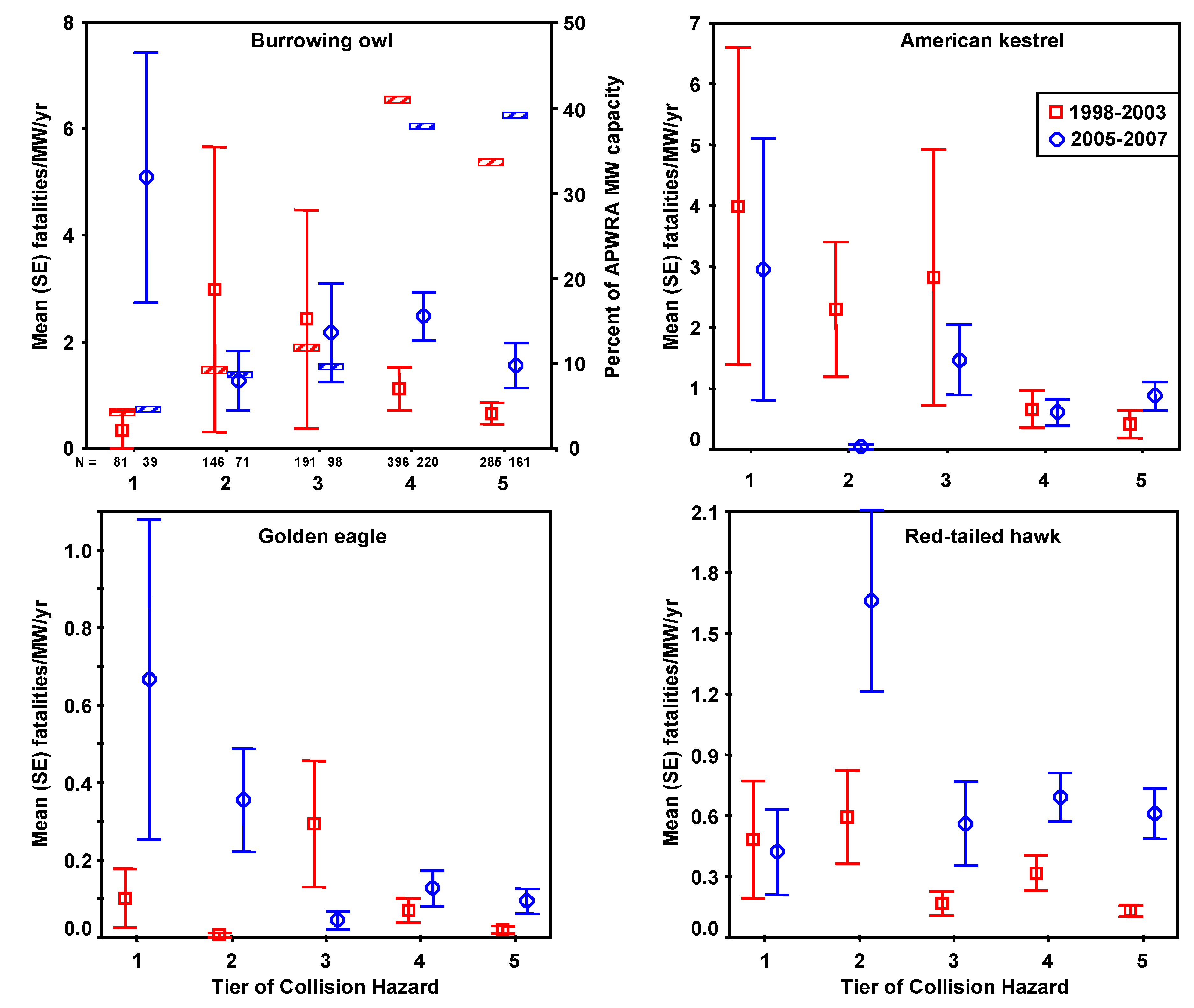
Fatality rates were expressed as the number of fatalities per MW per year, where MW was the rated power output of the wind turbines composing a row of wind turbines, and the number of years or fractions of a year were the time spans over which searches were performed at that wind turbine row. Fatality rates were based on fatalities occurring ≤90 days before discovery, and 0.25 years was added to the number of years used in each fatality rate calculation to represent the time period when fresh carcasses could have accumulated prior to the first search. We adjusted fatality rates, FA, for carcasses not found due to searcher detection error and scavenger removal [2]:
Energies 02 00915 i001
where FU was unadjusted fatality rate, p was the average proportion of fatalities found by searchers during searcher detection trials across the U.S. [15], and RC was the average cumulative proportion of carcasses remaining since the last fatality search, assuming wind turbines deposit carcasses steadily through the search interval. Preliminary RC values were estimated using reports of scavenger removal trials across the U.S. [15]:
Energies 02 00915 i002
where Ri was the proportion of carcasses remaining by the ith day into a scavenger removal trial and corresponding with days since the last search during fatality monitoring, and I was the average search interval (days). We looked up RC values in [15, App.], but we note that new approaches to scavenger removal trials have been generating faster removal rates (Smallwood et al., manuscript in preparation). Searcher detection and scavenger removal rates varied across the U.S., but not nearly to the degree they varied by typical body size categories and by whether raptors or nonraptors [15]; nevertheless, multiple sources of error and bias have yet to be characterized.

3.2. Mapping Burrowing Owl and Mammal Burrows for Model Development

We mapped burrows of mammals and burrowing owls using a Trimble Pro-XR GPS within 90 m of 571 wind turbines composing 70 rows that were also monitored for bird fatalities during 1999–2003. We selected turbine rows to represent the existing variation in documented raptor fatality rates, physiographic conditions, and levels of effort directed toward ground squirrel control. We mapped the approximate centroids of ground squirrel burrow systems using a pacing method to separate burrow systems when continuity of sign rendered inter-burrow system distinctions difficult [16]. Ground squirrel burrow systems can contain multiple adults. We walked parallel transects 0, 15, 30, 45, 60, 75, and 90 m away from the turbine row, thus covering increasingly larger areas around the turbine rows.
Areas intervening turbine rows were also mapped in some turbine fields, including: (1) 66 ha with 131 Micon 65-kW turbines arranged in seven rows near Mountain House; (2) 57 ha with 120 Vestas 100-kW turbines in eight rows just south of Old Altamont Road in the central portion of the APWRA; (3) 21 ha with 29 Enertech turbines arranged in five rows near the Seawest office; (4) 14 ha with 18 Micon 65-kW wind turbines in five rows off Midway Road; (5) 15 ha with 15 Flowind 150-kW and Bonus 150-kW turbines in four rows on the Elworthy Ranch; (6) 26 ha with 24 Bonus 120- and 150-kW turbines in four rows on the Elworthy Ranch; and, (7) 32 ha with 30 Bonus 120-kW turbines in five rows on the Elworthy Ranch. Intervening areas were mapped between other turbine rows, as well, but these were relatively small areas.
Burrowing owl burrows were identified after burrowing owls flushed from the burrow or by sign. Sign included pellets, whitewash, shed feathers, and/or nest displays composed of cattle dung, toad skins, lizard carcasses, decapitated small mammals, and/or arranged sticks. Not all burrows mapped were nest burrows, but only 1 of ≥2 burrows was mapped when burrows occurred ≤25 m apart, which was closer than the closest inter-nest distance reported elsewhere [17].

3.3. Spatial Models to Predict Burrowing Owl Locations

We mapped burrowing owl burrows as point features in ArcMap GIS layered onto a digital elevation model (DEM). We characterized the location of each burrowing owl burrow by slope aspect, slope grade, rate of change in slope, direction of change in slope, and elevation. These variables were also used to generate raster layers of the study area, one raster expressing the aspect of the corresponding slope (hereafter referred to as ‘slope aspect’), and the other expressing whether the landscape feature was tending toward convex versus concave orientation. These features were defined using geoprocessing.
The United States Geological Survey (USGS) 10-m DEM was used as a starting point for characterizing the terrain of the Altamont Pass. To replace poorer quality data across about 25% of the study area, geo-referenced USGS 7.5’ digital raster graphics (DRG) were used with GIS to capture the contour lines (hypsography). These contour vectors were then run through ESRI’s Topograph tool to create a 10-m DEM, which was inserted into the existing USGS 10-m DEM. Elevation was assigned to each grid cell according to its centroid.
From the final DEM of the Altamont Pass region, the statistical analyses were limited (masked) to data within the areas searched for ground squirrel and burrowing owl burrows. The resulting analytical grid was composed of 187,908 10 × 10 m2 cells. The analytical grid was used to develop and test predictive models, which were later projected across the 2,281,169 grid cells composing the APWRA. The analytical grid was not selected randomly from within the APWRA because the focus of the burrow mapping was on raptor prey species nearby the wind turbines, most of which were placed along ridge crests and ridgelines between peaks and valley bottoms. Thus, some landscape features within the analytical grid were disproportional to their occurrence within the APWRA, such as ridge crests. Model predictions will be more reliable for landscape features represented within the analytical grid than for landscape features typically farther away from wind turbines.
Figure 3. 
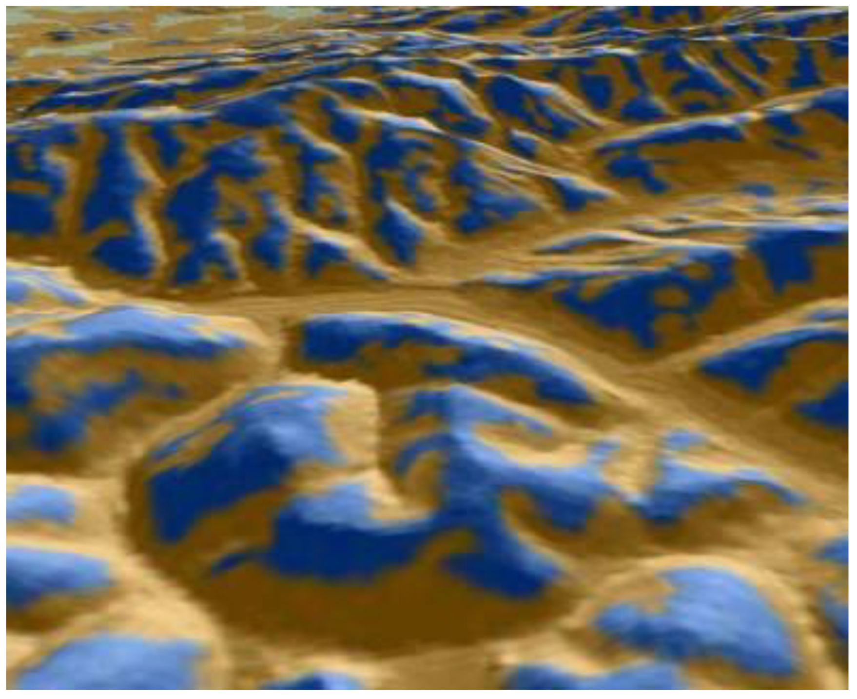
Ridge and valley features expressed as blue and gold, respectively, and typical of convex-trending groups of DEM grid cells (ridges) and concave-trending groups of grid cells (valleys).
Energies 02 00915 g003
We used the Curvature function in the Spatial Analysis extension of ArcGIS 9.2 to calculate the curvature of a surface at each cell centroid. A positive curvature indicated the surface was upwardly convex at that cell, a negative curvature indicated the surface was upwardly concave, and a value of zero indicated the cell surface was flat. The curvature data (–51 to 38) were classified using the NaturalBreaks (Jenks) function with three classes of curvature–convex, concave and mid-range. The break values were visually adjusted to minimize the size of the mid-range class. We used a series of geoprocessing steps called ‘expand,’ ‘shrink,’ and ‘regiongroup,’ as well as ‘majority filter tools’ to enhance the primary slope curvature trend of a location. The result was a surface almost exclusively defined as either convex or concave (Figure 3). The convex surface areas consisted primarily of ridge crests and peaks, hereafter referred to as ridges, and the concave surface areas consisted primarily of valleys, ravines, ridge saddles and basins, hereafter referred to as valleys.
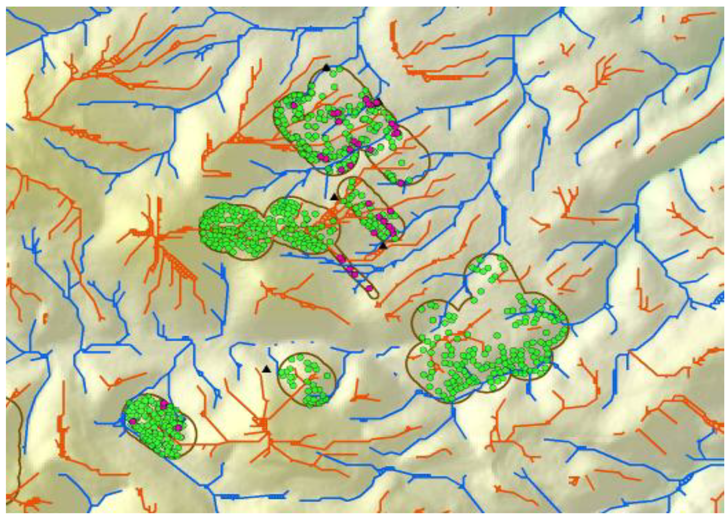
Line features representing the estimated average centers of ridge crests and valley bottoms (Figure 4) were derived from the following steps. ESRI’s ‘Flowdirection’ function was used to create a flow direction from each cell to its steepest down-slope neighbor, and then the ‘Flowaccumulation’ function was used to create a grid of accumulated flow through each cell by accumulating the weight of all cells flowing into each down-slope cell. A valley started where 50 upslope cells had contributed to it in the Flowaccumulation function, and a ridge started where 55 cells contributed to it. The flowdirection and flowaccumulation functions were applied to the ridges by multiplying the DEM by −1 to reverse the flow. Line features that represented ridges and valley bottoms were derived from ESRI’s gridline and thin functions, which feed a line through the centers of the cells composing the valley or ridge. Thinning put the line through the centers of groups of cells ≥40 in the case of valleys.
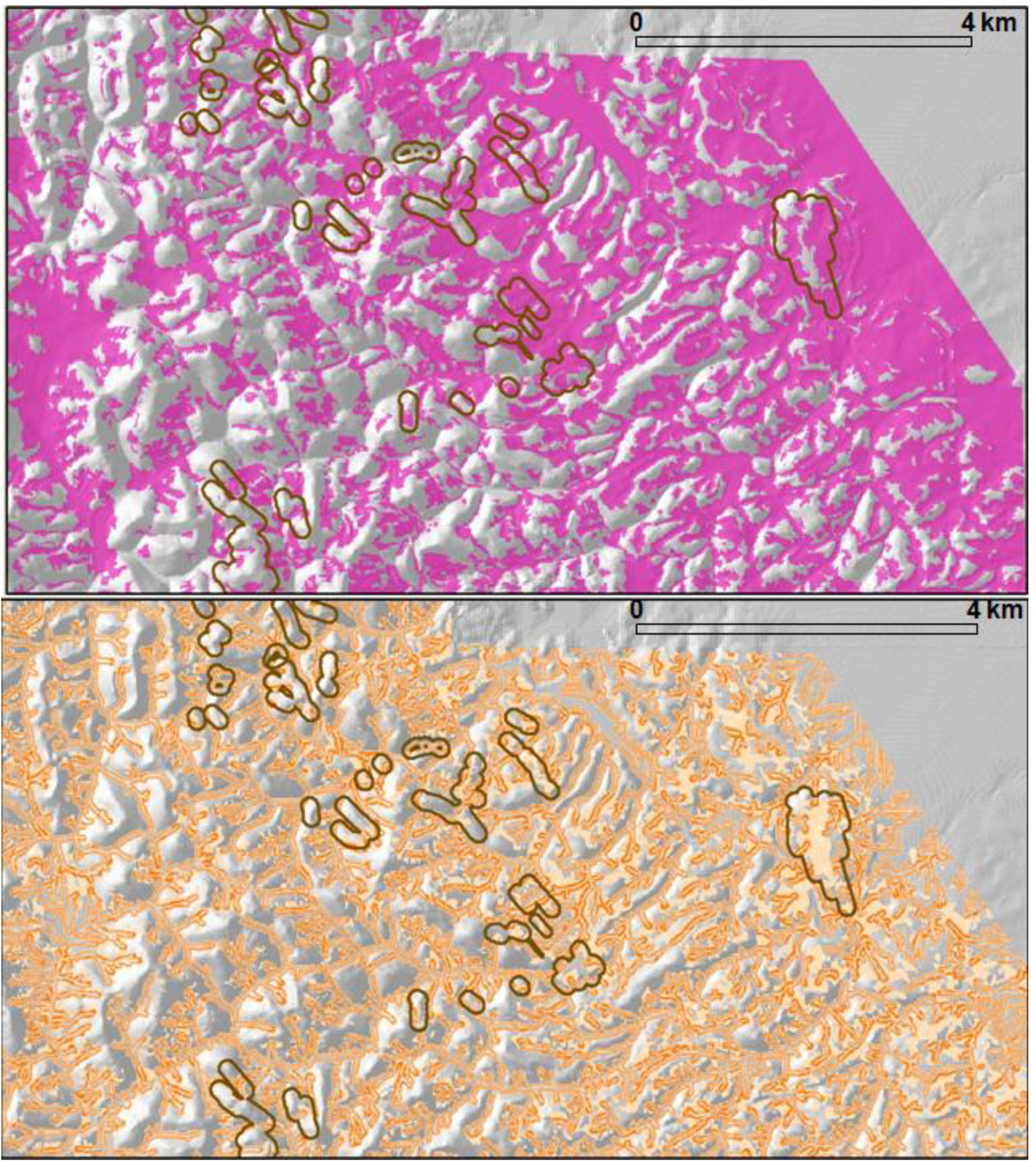
Figure 4. 
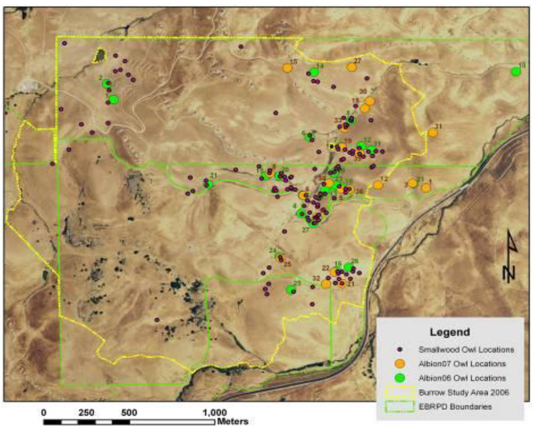
Line coverages of ridge tops (orange) and valley bottoms (blue) following multiple geoprocessing steps assessing trends in neighboring DEM grid cells. Polygons enclose areas around wind turbines where burrow systems of ground squirrel (green) and burrowing owls (magenta) were mapped to develop predictive models.
Energies 02 00915 g004
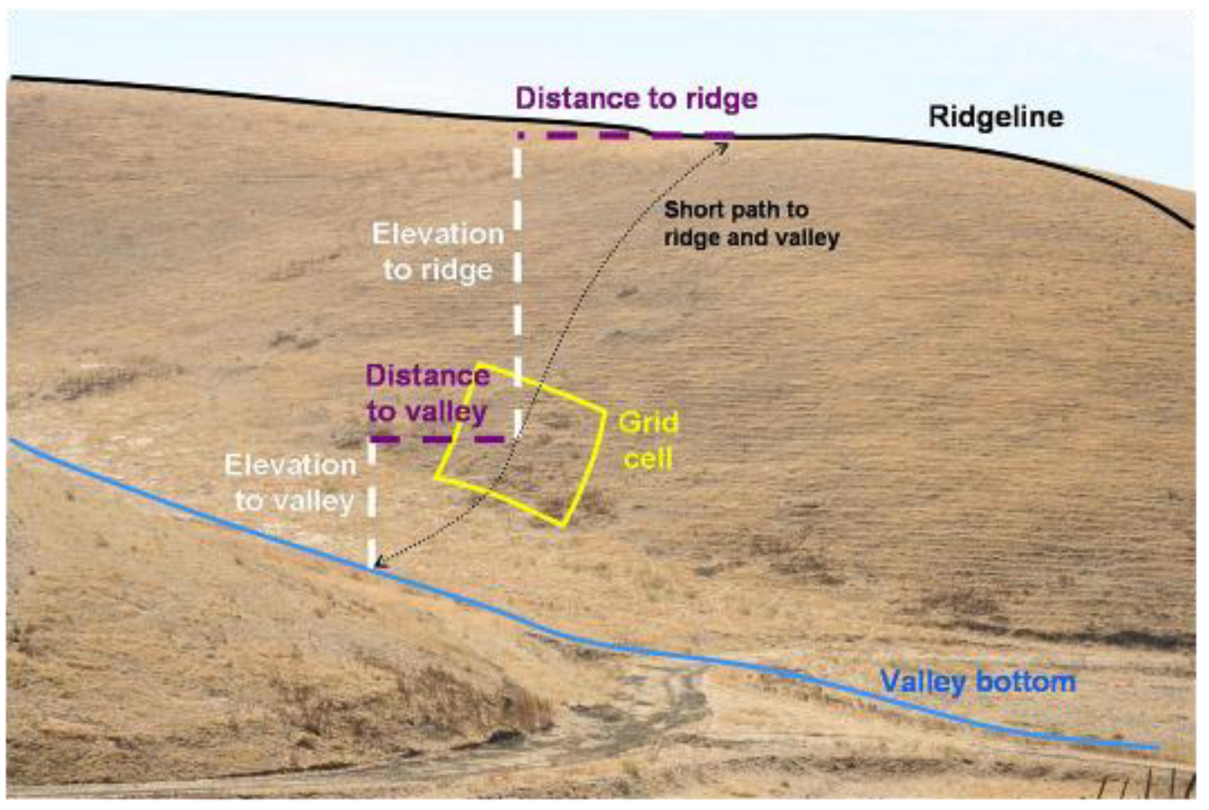
The horizontal distance (m) of each DEM grid cell was then measured from the nearest valley bottom and the nearest ridgeline, referred to as distance to valley and distance to ridge, respectively (Figure 5). These distances were measured from the DEM grid cell to the closest grid cell of a valley bottom or ridgeline, respectively, not including vertical differences in position. The total distance across the underlying slope was the sum of the distance to the valley bottom and the distance to the ridgeline, and expressed the size of the slope (total slope distance). The DEM grid cell’s position in the slope was also expressed as the ratio of the distance to the valley and the distance to the ridge, referred to as the distance ratio. This expression of the grid cell’s position on the slope removed the size of the slope as a factor.
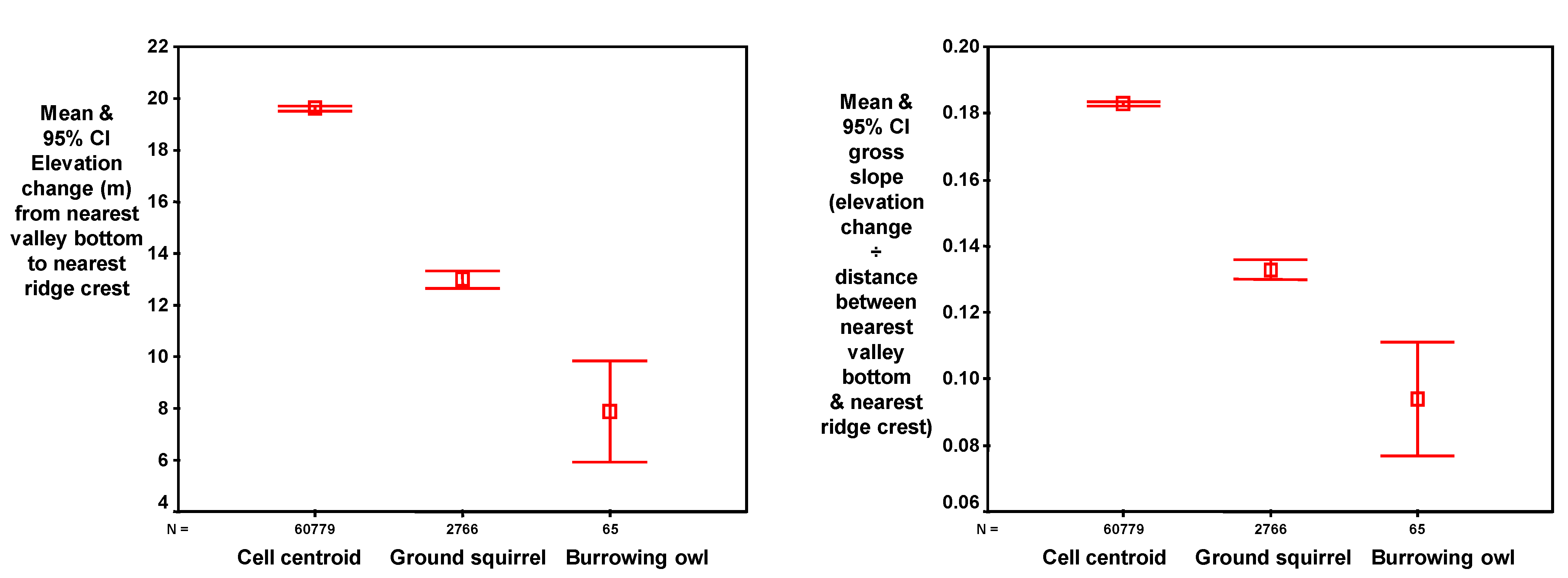
The vertical differences between each DEM grid cell and the nearest valley bottom and nearest ridgeline were referred to as elevation difference (Figure 5), and this measure also expressed the size of the slope. In addition to the trend in slope grade at each DEM grid cell, the gross slope was measured as the ratio of elevation difference and total slope distance (Figure 5). The DEM grid cell’s position on the slope was also expressed as the ratio of the elevation differences between the grid cell and the nearest valley and the grid cell and the nearest ridge, referred to as elevation ratio.
Figure 5. Example depiction of how slope attributes were measured from 10 m2 DEM grid cells. The elevation difference was the Elevation to valley + Elevation to ridge, and elevation ratio was Elevation to valley ÷ Elevation to ridge. Total slope distance was Distance to valley + Distance to ridge, and distance ratio was Distance to valley ÷ Distance to ridge. Gross slope was elevation difference ÷ total slope distance. The hypothetical grid cell overlaps a burrowing owl burrow located on another project site in the APWRA.
Energies 02 00915 g005
Each DEM grid cell was classified by slope aspect according to whether it faced north, northeast, east, southeast, south, southwest, west, northwest, or if it was on flat terrain. For analysis slope aspect was aggregated into five categories: northeast and east, southeast and south, southwest and west, northwest and north, and no aspect (flat terrain). Each grid cell was categorized as to whether its center on the landscape was windward, leeward or perpendicular to the prevailing southwest and northwest wind directions as recorded during earlier behavior observation sessions [9,18].
Log10 and natural log transformations were used to better fit normal distributions, and then chi-square tests for association and principal components analysis (PCA) were used to further understand how the variables related to burrowing owl burrow locations and to each other. To minimize the effects of confounding, no more than one predictor variable was selected from each principle component for any model developed to classify grid cells according to whether they supported burrowing owl burrows. The first modeling approach used discriminant function analysis (DFA), and the second used fuzzy logic [19,20]. Both produced likelihood surface areas, one referred to as the DFA surface and the other as FL surface. The performance of each model was based on the lowest number of predictor variables, the smallest portion of the study area occurring within the likelihood surface area, and the most number of mapped burrows occurring within the likelihood surface.
Log10 distance to valley and elevation difference were the two variables used in fuzzy logic to predict the likelihood of each grid cell containing a burrowing owl burrow (Table 1). These two variables were selected from a pool of candidates, based on relatively larger magnitudes of differences between mean values where burrowing owls were and were not found, and based on their relatively lower level of shared variation as judged from examination of a correlation matrix and the output from principal components analysis.
Table 1. Fuzzy logic membership functions of grid cells belonging to the set of cells with burrowing owl burrows, based on a sample of 187,908 10 × 10 m2 grid cells. For log10 distance to valley, mean = 1.27302, SE = 0.11455, and SD = 0.46176, and for elevation difference, mean = 7.5846 and SE = 0.97564.
Value of variable Y for ith grid cellBasis of membership functionMembership function of grid cell belonging to set with a burrowing owl burrow
Y = log10 distance to valley
1.15847 < Y < 1.38757Within 1 SE of mean1
0.81126 ≤ Y ≤ 1.158471 SD to 1 SE < mean0.5 × (1 – cos(π × (Y − 0.81126) ÷ (1.15847 − 0.81126)))
1.73478 ≥ Y ≥ 1.387571 SD to 1 SE > mean0.5 × (1 + cos(π × (Y − 1.38757) ÷ (1.73478 − 1.38757)))
Y < 0.81126 or Y > 1.73478>1 SD away from mean0
Y = elevation difference
5.63332 < Y < 9.53588Within 1 SE of mean1
3.68204 ≤ Y ≤ 5.63332Within 4 × SE; 2 × SE < mean0.5×(1 − cos(π × (Y − 3.68204) ÷ (5.63332 − 3.68204)))
11.48716 ≥ Y ≥ 9.53588Within 4 × SE; 2 × SE > mean0.5×(1 + cos(π × (Y − 9.53588) ÷ (11.48716 − 9.53588)))
Y < 3.68204 or Y > 11.48716>4 SE; away from mean0
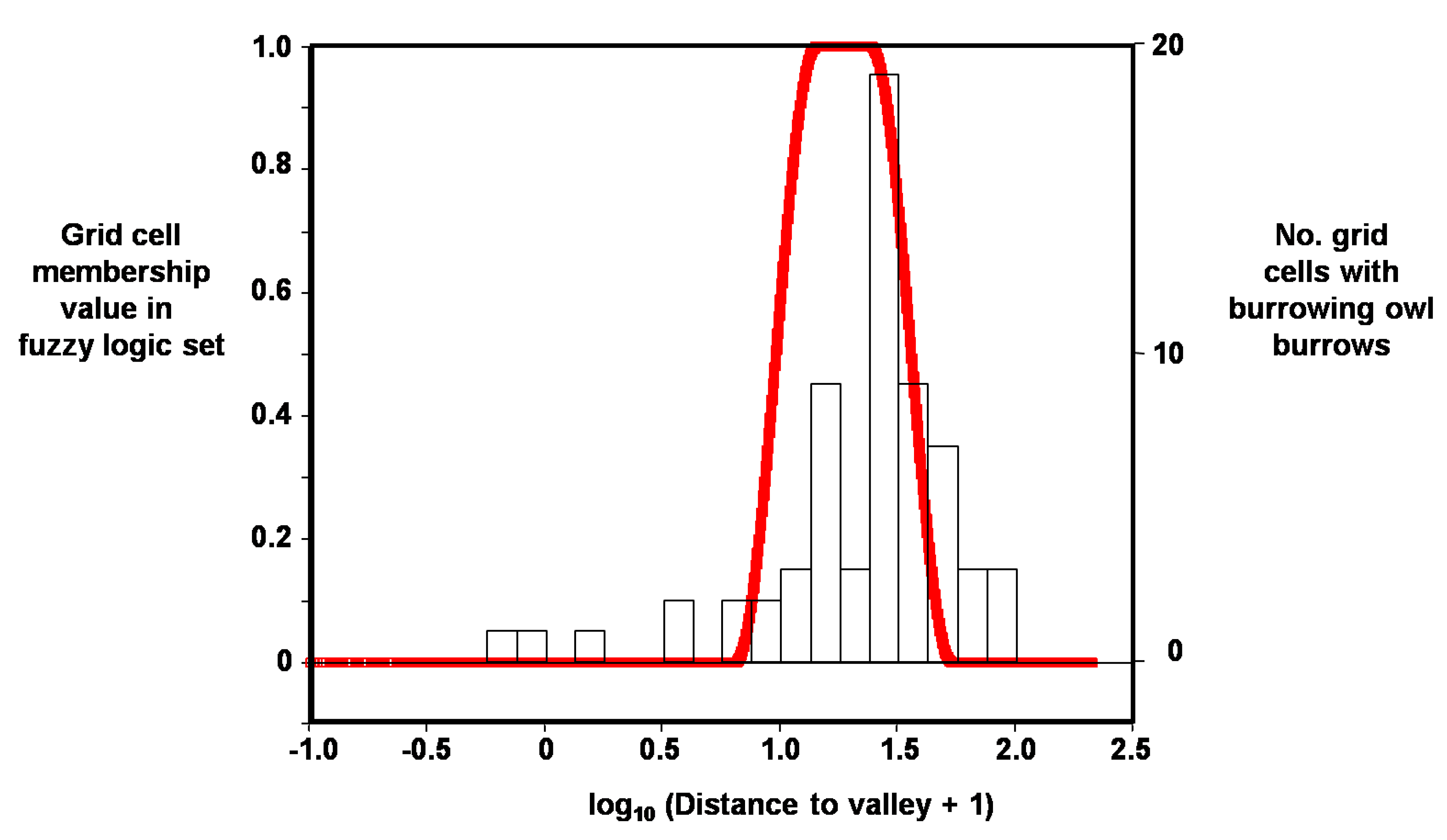
Based on log10 distance to valley, the grid cell’s membership value in the burrowing owl burrow set was multiplied by 2.55 × 100, and based on elevation difference it was multiplied by 100 in order to obtain a value range that was easier to report and interpret. These two products were added and all sum values >70 were used to obtain the fuzzy logic surface because 70 appeared to be a natural break in the frequency distribution.
Figure 6. Example distribution of membership values in fuzzy logic set (red line), in this case for grid cells containing burrowing owl burrows as a function of log10 distance to valley.
Energies 02 00915 g006

3.4. Spatial Model Validation Using Burrowing Owl Locations in Vasco Caves

From August through November 2006, we used a Trimble Geo-XT GPS to map the approximate centers of burrow systems of burrowing owls, ground squirrels, and other mammals in Vasco Caves Regional Preserve [14]. We used the pacing method described earlier along transects spaced about 12 to 15 m apart on 381 ha (70%) of the Preserve. Burrowing owl burrows mapped included burrows used for both nesting and refuge.
A separate effort was made to specifically map burrowing owl nesting burrows. Biologists searched for burrowing owls and their nest burrows from 33 observation points in 2006 and 39 points in 2007, using 10 × 40 binoculars and a 25 × 60 spotting scope from both inside and outside an automobile. They performed 15 surveys (54 hours) from 24 May to 2 August 2006, and 11 surveys (44 hours) from 3 April to 27 June 2007. Each year, 11 surveys were initiated during morning, generally lasting from about 08:00 hours to 13:00 hours. Nest burrows had a breeding pair in attendance during repeat surveys. To represent nest productivity, the maximum number of emergent juveniles between 2 and 4 weeks old was recorded. Results from both the general burrow mapping survey and the nesting owl burrow survey were used in this analysis.
Mapped burrowing owl burrows were characterized as point features in ArcMap GIS and layered onto our DEM of the study area. The location of each burrow was examined for overlap with our predictive models developed using data from other parts of the APWRA. The analytical grid for the burrow mapping area in the Vasco Caves study area consisted of 38,139 10 × 10 m2 cells.

3.5. Non-Spatial Models to Predict Burrowing Owl Fatalities

We developed a simple rating system to score the collision hazard of each of the 4,074 wind turbines searched for fatalities during 1998–2003. We selected specific conditions to be rated for collision hazard following chi-square tests for association between fatalities and measured environmental variables and wind turbine attributes [9]. Test results leading to conditions we rated were those that were (1) significant, (2) based on expected χ2 cell values mostly >5, (3) exhibited sensible gradients in measures of effect (i.e., relating observed to expected values) along a continuum such as elevation or rotor diameter, and (4) reasonably orthogonal.
Using magnitudes of observed ÷ expected ratios from the χ2 tests, we scored wind turbines for their collision hazard to four raptor species that are the most often killed in the APWRA, because these species were the foci of mitigation measures required by Alameda County’s conditional use permits issued to the wind turbine companies (Table 2). Burrowing owls contributed to this scoring system, but the other three species obviously also affected the scores. The sum scores were aggregated into 4 groups per species, and then the aggregated scores were subjected to conditional statements (Table 3). The conditional statement considered natural breaks in ranges of sum scores specific to each species.
Table 2. Rating system to score APWRA wind turbines for collision hazard to four select species of raptor.
Wind Turbine ConditionScore
Rotor plane swept/s < 2,142 m21
Supporting tower is tubular or vertical axis1
Non-functional or next to derelict turbine or vacant tower1
Not part of a wind wall1
At the end of a turbine row1
In a canyon1
At or below 235 m elevation1
In valley (trending toward upwardly convex)1
Burrowing owl sum score_____ (10 possible)
Low reach of blades 8 to 9.6 mabove ground1
Fewer than 24 other turbines within 300 meters1
At the edge of a local cluster of turbines1
Not part of a wind wall1
At the end of a turbine row1
On a ridgeline1
In a canyon1
On steep slopes, >14°1
On slopes windward to one prevailing wind direction (NW or SW) and perpendicular to the other direction1
Golden eagle sum score_____ (9 possible)
At the end of a turbine row1
Fewer than 13 other turbines within 300 meters1
At the edge of a local cluster of turbines1
In a canyon1
On a ridgeline or ridge saddle1
On a northwest- or south/southeast-facing slope1
At or above 385 m elevation1
Red-tailed hawk sum score_____ (6 possible)
Rotor plane swept/s > 3,285 m21
On ridgeline or ridge saddle1
Below 135 m or above 385 m elevation1
American kestrel sum score_____ (3 possible)
Table 3. Conditional statements applied to the rating system for collision hazard to identify tiers of wind turbines grading from most hazardous (Tier 1) to least hazardous (Tier 5), where GOEA = golden eagle, RTHA = red-tailed hawk, BUOW = burrowing owl, and AMKE = American kestrel.
Index scoresTierNo. of turbines
GOEAOperatorRTHAOperatorBUOWOperatorAMKE
4and4and≥1and≥1122
≥1or≥1and≥3and≥31124
≥3or≥3and≥4or≥4175
4and≥3and---and---245
---and---and≥3and≥22235
≥3and≥3and≥2and≥13149
≥2and≥3and≥1and---3323
≥3or≥3or≥3and---4603
Else the turbine was assigned to Tier 552,498

4. Results

4.1. Landscapes Used to Develop and Validate Predictive Spatial Models

Principal components analysis, using a correlation matrix and varimax rotation, explained 82% of the variation in predictor variables measured among APWRA-wide grid cells masked for model development, and it also explained 82% of the variation in predictor variables measured among the grid cells in Vasco Caves used for model validation (Table 4).
Table 4. Principal Components following varimax rotation in PCA, showing only those rotated factor loadings >0.1.
VariableComponent 1Component 2Component 3
APWRAVascoAPWRAVascoAPWRAVasco
ln Distance ratio0.9840.979
ln Elevation ratio0.9070.9210.133
log10 Distance to ridge−0.872−0.8510.3120.332
log10 Distance to valley0.8000.8070.4800.472
Gross slope0.9080.9090.175
Elevation difference0.8310.7750.4400.549
Slope (percentage)−0.1190.8290.745
Elevation0.2140.4370.6270.234−0.191−0.211
log10 Total slope distance0.1590.9270.959
Component 1 can be interpreted as position on the slope, which loaded stronger on elevation at Vasco Caves. Component 2 can be interpreted as the slope’s rate of change, i.e., steepness. Component 3 can be interpreted as the slope’s size. Only one variable with a high loading was used from each component for subsequent predictive model development, though all variables and transformed variables were tested for a relationship with burrowing owl burrows.

4.2. Burrowing Owl Burrows Contributing to Model Development and Validation

We mapped the locations of 65 burrowing owl burrows found during systematic searches of plots throughout the eastern, central, and southern portions of the APWRA in 1999–2003. While mapping mammal burrows in Vasco Caves during fall 2006, we detected 143 burrowing owl burrows used for nesting and refuge (Figure 7). Biologists performing directed breeding pair surveys determined burrowing owls were nesting in 25 (76%) of 33 burrows in use by pairs in 2006, and in 21 (54%) of 39 burrows in use in 2007 (Figure 7). Breeding pair density of burrowing owls on the project site was ≥4.61 per 100 ha in 2006 and 3.87 per 100 ha in 2007, both within the confidence interval predicted by an empirical model [3]. One or more young emerged from 19 of 25 breeding pairs for nest success of 76% in 2006, and one or more young emerged from 12 of 21 breeding pairs for nest success of 57% in 2007. Productivity was 3.44 juveniles/pair (N = 86 young) in 2006 and 1.95 juveniles/pair (N = 41 young) in 2007.
A year of fatality monitoring among the 21.9 MW of wind turbines in Vasco Caves detected 10 burrowing owl fatalities, all at turbines we rated as Tier 1 and Tier 2 (most hazardous). We estimated 17.7 burrowing owls were killed annually in Vasco Caves (Smallwood et al. manuscript in prep.), or about 13% to 21% of the total annual population at Vasco Caves. However, we do not know whether or to what degree this level of fatalities affects the local population.
Figure 7. Distribution of burrowing owl burrows used in Vasco Caves Regional Preserve for nesting in 2006 (green circles) and 2007 (orange circles), and for refuge in 2006 and 2007 (maroon circles).
Energies 02 00915 g007

4.3. Burrowing Owl Relationships with Ground Squirrels and Slopes

Compared to the average grid cell, those with ground squirrel burrow systems and burrowing owl burrows were successively lower on the slope (Table 5, Figure 8), on successively smaller slopes (Figure 9A) and on successively shallower slopes (Figure 9B). Burrowing owls did not occupy ground squirrel burrows at random, but rather selected burrows within a relatively narrow range of topographic conditions.
Nearly all measured slope attributes differed between sets of grid cells with and without burrowing owl burrows (Table 6). Grid cells with both nest and refuge burrows averaged about half the distance to valley compared to grid cells without burrows, and grid cells with nest burrows in Vasco Caves averaged 59% of distance to valley compared to other grid cells. Differences in multiple other measured variables indicated that burrowing owl burrows were on average nearer the valley bottoms than they were the ridge crests, at lower elevations than where burrowing owl burrows were not found, and were on smaller, shallower slopes (Table 6).
Table 5. Mean comparisons among sets of grid cells with ground squirrel burrow systems, burrowing owl burrows, and neither ground squirrel nor burrowing owl burrows (empty cells) in the portions of the APWRA used to develop predictive models of burrowing owl burrow locations. Post-hoc least significant difference tests were denoted by a for tests between empty cell and ground squirrel, b for empty cell and burrowing owl, and c for ground squirrel and burrowing owl, and the overall ANOVA df = 1,187,907. Sample sizes were n = 185,077 for empty cells, n = 2,766 for cells with ground squirrels, and n = 65 for cells with burrowing owls.
Predictor variableMeanANOVA F-valueLeast-significant differences
Empty cellGround squirrelBurrowing owl
Distance to valley61.8046.3829.25466.80**abc
Distance to ridge42.1246.6945.0963.31**a
Total slope distance103.9393.0674.34353.47**abc
Distance ratio5.403.331.4592.27**ab
Elevation192.55140.75143.43774.58**ab
Elevation difference17.1212.987.71176.64**abc
Elevation ratio5.432.861.20274.78**ab
Gross slope (%)15.8713.289.14112.26**abc
Slope at grid cell (%)18.8917.1213.3857.23**abc
Principal component 10.0049−0.3128−0.5301146.83**ab
Principal component 20.0053−0.3433−0.6078178.02**abc
Principal component 30.0027−0.1650−0.767857.53**abc
Figure 8. Mean and SE of percent of elevation from the bottom to the top of the slope on which the grid cell is located within Vasco Caves Regional Preserve. On average, ground squirrel burrow systems were lower on the slope than the average grid cell, and burrowing owl burrows, including nest burrows, were lower yet.
Energies 02 00915 g008
Figure 9. Compared to the average empty grid cell, those with ground squirrel burrows were relatively low on the slope (A), those with burrowing owl burrows were lower still (A), and those with ground squirrel burrows were on shallower slopes (B), and burrowing owl burrows were on even shallower slopes (B).
Energies 02 00915 g009
Table 6. Mean comparisons between sets of grid cells where burrowing owl burrows were not found and where they were found. Significance of ANOVA tests was denoted by *for P < 0.05 and ** for P < 0.005.
Predictor variableBurrowing owl burrowsANOVA F-value
Not foundFound
MeanSDMeanSD
Refuge & nest burrows APWRA-wide
Distance to valley (m)61.5837.2929.2519.1248.84**
Distance to ridge (m)42.1929.9445.0918.400.61
Total slope distance (m)103.7730.1674.3422.0161.86**
ln Distance ratio0.461.63−0.531.1823.69**
Elevation (msl)191.7997.35143.4338.1816.04**
Elevation difference (ridge − valley)17.0612.187.718.0238.30**
Gross slope (%)16109730.85**
Slope at grid cell (%)18.8612.1913.388.1713.12**
ln Elevation ratio0.601.67−0.270.8717.52**
PC 1, position on slope0.001.00−0.530.6218.27**
PC 2, slope steepness0.001.00−0.610.6324.02**
PC3, slope size0.001.00−0.770.9338.34**
Refuge & nest burrows in Vasco Caves
Distance to valley (m)59.0740.6034.7323.9747.02**
Distance to ridge (m)59.5341.8985.8028.9051.40**
Total slope distance (m)118.6040.99120.5333.890.29
ln Distance ratio0.011.82−1.121.0050.71**
Elevation (msl)199.1045.87147.0226.43168.75**
Elevation difference (ridge − valley)25.7414.8821.4711.6910.76*
Gross slope (%)221018817.26**
Slope at grid cell (%)27.0712.5523.879.758.50*
ln Elevation ratio0.101.95−1.171.2555.85**
PC 1, position on slope0.001.00−0.740.5572.33**
PC 2, slope steepness0.001.00−0.470.7429.26**
PC 3, slope size0.001.000.270.749.48*
Nest burrows in Vasco Caves
Distance to valley (m)59.0040.5843.2733.316.16*
Distance to ridge (m)59.6041.8883.3732.7313.19**
Total slope distance (m)118.6040.97126.6440.761.58
ln Distance ratio0.011.82−1.011.5712.83**
Elevation (msl)198.9845.90143.5621.3959.77**
Elevation difference (ridge – valley)25.7314.8724.8312.670.15
Gross slope (%)22102071.74
Slope at grid cell (%)27.0612.5424.6110.631.56
ln Elevation ratio0.101.95−1.031.3613.74**
PC 1, position on slope0.001.00−0.700.7519.98**
PC 2, slope steepness0.001.00−0.340.694.66*
PC 3, slope size0.011.00−0.210.966.55*

4.4. Spatial Model to Predict Burrowing Owl Locations

The most efficient DFA models were comprised of fewer variables that correctly classified a higher percentage of grid cells where burrowing owl burrows were found (Table 7). Elevation difference contributed to the most efficient models, as did total slope distance and natural log elevation ratio. Slope size contributed most to the DFA model developed from the PCA scores, followed by slope steepness and position on the slope. According to this model, grid cells predicted to overlap burrowing owl burrows also overlapped smaller and shallower slopes closer to the valley bottom.
The most reliable assessment of each model in Table 7 was the percent correct classification of grid cells with burrowing owl burrows, because grid cells without burrowing owl burrows could have had owl burrows in the past and might have them in the future (see Figure 7). Burrowing owls shift burrow locations occasionally, and population turnover will also result in a dynamic spatial distribution of burrows.
Table 7. The most efficient discriminant function models of grid cells predicted to include burrowing owl burrows, as well as a DFA model estimated from the PCA scores. All three models were significant (P < 0.0001).
Discriminant Functions (standardized canonical discriminant function coefficients)Percent correct classification of grid cells
Where burrowing owl burrows were foundTotal
Total slope distance (0.77), Elevation difference (0.35)84.667.4
Elevation difference (0.82), ln Elevation ratio (0.50)87.762.3
Position on slope (0.48), Slope steepness (0.55), Slope size (0.69)72.372.8
The DFAs performed reasonably well by correctly predicting 72% to 88% of the grid cells with burrowing owl burrows, but large numbers of grid cells were predicted to overlap burrowing owl burrows. One DFA model correctly predicted 88% of known burrow sites, but also predicted that 38% of the study area would contain burrowing owl burrows (Figure 10A).
Figure 10. Areas within part of the APWRA predicted to be selected by burrowing owls for burrow locations based on a Discriminant Function Model (A, magenta) and based on a Fuzzy Logic Model and surface values >70 (B), where the darker orange depict strongest prediction (bottom). Boundaries of some burrow mapping areas are shown by dark lines.
Energies 02 00915 g010
Based on our DFA model, the combinations of variables in Table 7 performed about as well as elevation difference and log10 distance to valley using fuzzy logic. These were selected from different PCs and shared little variation (r = 0.27), so they were reasonably orthogonal. Of the 65 burrowing owl burrows in the APWRA study area, 57 (88%) were located on the FL surface based on FL values >10, composing 52% of the study area. Burrowing owl burrows were associated with the fuzzy logic surface (χ2 = 33.17, df = 1, P < 0.001), and were mapped in it 1.69 times other than expected, i.e., Observed ÷ Expected = 1.69.
Of the 65 burrowing owl burrows compared to GIS raster layers, 53 (81.5%) were located in the FL surface with values >70. This likelihood surface was 43.2% of the study area (Figure 10B). Burrowing owl burrows were associated with the fuzzy logic surface (χ2 = 38.18, df = 1, P < 0.001), and were mapped in the FL surface 1.89 times other than expected.

4.5. Spatial Model Validation Using Burrowing Owl Locations in Vasco Caves

The FL surface developed from data collected in other parts of the APWRA correctly predicted the locations of most of the burrowing owl burrows found in Vasco Caves (Figure 11). The FL surface covered 40.9% of the burrow study area in Vasco Caves, but overlapped 69% of burrowing owl burrows found during foot searches in 2006. These burrows overlapped the FL surface 1.68 times other than expected. Of the nest burrows that were mapped, 63% overlapped the FL surface, or 1.55 times other than expected. Additionally, 61% of the juveniles produced from monitored nest burrows were from the FL surface, or nearly 1.5 times other than expected.
Figure 11. Most of the mapped burrowing owl burrows at Vasco Caves overlapped the fuzzy logic surface depicted here in shades of purple.
Energies 02 00915 g011

4.6. Relation of Predicted Burrowing Owl Locations to Wind Turbine Fatalities

Among all APWRA wind turbines, 16.4% (89.6 MW) were in and 83.6% (456.2 MW) were out of the DFA surface area, and the same percentages characterized the turbines that were searched. Burrowing owl fatalities were on the DFA surface 1.77 times other than expected (Table 8). The DFA surface also associated with disproportionately more wind turbine-caused fatalities of red-tailed hawk, mallard, western meadowlark, and mourning dove (Table 8), indicating turbines moved from this surface would benefit multiple species.
Among all APWRA wind turbines, 27.3% (149.7 MW) were in and 72.7% (398.0 MW) were out of the FL surface area based on surface values >70 (this value chosen as a natural break in surface values). Among searched wind turbines, 22% of the rated capacity was in the FL surface, and burrowing owl fatalities were in the FL surface 1.95 times other than expected (Table 8). The FL surface also associated with disproportionately more wind turbine-caused fatalities of western meadowlark and mourning dove (Table 8).
Adjusted fatality rate estimates were greater for most bird species within the FL surface during both 1998–2003 and 2005–2007 (Table 9). The fatality rates of burrowing owls and all raptors as a group were twice as high on the FL surface compared to off the FL surface in 1998–2003, but these differences lessened in 2005–2007.
Table 8. Fatalities off and on the sampled portions of the DFA and FL (values >70) surfaces across the APWRA, where the rated wind power capacity of turbines was 364.6 MW (84%) off the DFA surface and 71.5 MW (16%) on the DFA surface, and 340.0 MW (78%) off the FL surface and 97.8 MW (22%) on the FL surface. Significance of chi-square values were denoted by t for 0.10 > P > 0.05, * for P < 0.05, and ** for P < 0.005.
SpeciesLikelihood surface
Discriminant function analysisFuzzy logic
Observed fatalitiesObs ÷ ExpfatalitiesChi-squareObserved fatalitiesObs ÷ ExpfatalitiesChi-square
Golden eagleOff461.04360.92
On70.810.39181.271.09
Red-tailed hawkOff1660.941460.95
On461.324.38*671.182.03
American kestrelOff470.95370.87
On121.240.68221.443.31 t
Burrowing owlOff490.85340.73
On201.778.00**351.9517.78**
Barn owlOff390.95330.92
On101.250.58161.281.10
Great horned owlOff120.84110.83
On51.802.1171.581.65
MallardOff200.72210.86
On132.4112.76**121.492.30
Horned larkOff211.09150.90
On20.530.9981.360.87
Western meadowlarkOff700.88570.84
On251.616.85*391.568.42**
Mourning doveOff160.58160.66
On173.1529.74**182.1713.01**
RaptorsOff4030.943310.89
On1111.3210.20**1861.3820.92**
BirdsOff8280.866950.84
On3211.71112.03**4611.55101.66**
Table 9. Comparisons of adjusted fatality rate estimates within and outside fuzzy logic likelihood surfaces.
SpeciesFatality rates (Fatalities/MW/yr)
1998–20032005–2007
Off FL surfaceOn FL surfaceOff FL surfaceOn FL surface
MeanSEMeanSEMeanSEMeanSE
Burrowing owl0.8050.3541.6300.6971.7310.3002.3630.408
Golden eagle0.0880.0460.1210.0560.2100.0440.2280.111
Red-tailed hawk0.2990.0660.2700.0700.7030.0960.8100.129
American kestrel0.8390.2512.4141.3550.7240.1870.7510.184
Barn owl0.0500.0150.0640.0290.1940.0370.3000.093
Great horned owl0.0130.0060.0100.0050.0530.0280.0940.034
Mallard0.0750.0300.0810.0410.1200.0700.0490.037
Mourning dove0.0000.0000.0000.0000.0890.0420.1260.086
Western meadowlark3.2611.3792.0730.6682.9600.4353.5670.691
Raptors2.1020.7454.5172.2173.8180.8124.6801.048
Birds12.5106.00412.4055.70615.0013.83919.9705.643

4.7. Non-Spatial Models to Predict Burrowing Owl Fatalities

Estimated fatality rates corresponded with Tier classifications assigned to wind turbines based on collision hazard ratings for 3 of the 4 raptor species that were used to develop the Tiers (Figure 12). Fatality rates of burrowing owl were highest in Tier 2 and 3 turbines in 1998–2003, and were highest in Tier 1 turbines in 2005–2007. Fatality rates of American kestrel were highest in Tier 1–3 turbines in 1998–2003 and in Tier 1 and 3 turbines in 2005–2007. Fatality rates of golden eagle were highest in Tier 3 turbines in 1998–2003 and in Tier 1 and 2 turbines in 2005–2007. Fatality rates of red-tailed hawks were highest in Tier 2 turbines in 2005–2007. Turbines in Tiers 1–3 caused the highest fatality rates of these four raptor species, and composed 22% to 26% of the APWRA’s installed capacity.

5. Discussion

Both discriminant function analysis and fuzzy logic approaches produced predictive models of burrowing owl locations, and their likelihood surfaces were also where wind turbines killed disproportionate numbers of burrowing owls. The fuzzy logic approach was more predictive of burrowing owl fatalities, whereas the DFA approach was more predictive of fatalities of other bird species. Therefore, focused planning to minimize burrowing owl fatalities by carefully repowering the APWRA would benefit from using the FL approach combined with the rating system, whereas planning to minimize the fatalities of a larger suite of species would benefit from using the DFA approach combined with the rating system.
Figure 12. Mean fatality rates by collision hazard Tier classification for burrowing owl, American kestrel, golden eagle, and red-tailed hawk estimated from fatality monitoring in 1998–2003 and 2005–2007 in the Altamont Pass Wind Resource Area. Hatched bars in the top left graph represent percentages of the APWRA’s installed capacity in each Tier, e.g., Tier 1 turbines represented 4.4% and 4.7% of the APWRA’s installed capacity in 1998-2003 and 2005–2007, respectively.
Energies 02 00915 g012
Although burrowing owls rely heavily on ground squirrels for constructing their burrows, they were selective about which of the available ground squirrel burrow systems they used. Burrowing owls selected ground squirrel burrows on shallower, smaller slopes than average ground squirrel burrow locations, and toward the bottoms of slopes, but usually just above the flatter portions of terrain normally regarded as valley bottoms. In the APWRA burrowing owl burrows usually occur on portions of slopes where an ill-defined boundary exists between the valley bottom and the slope of the hill, an area we term the valley transition zone. The hypothetical grid cell in Figure 5 exemplifies the valley transition zone selected by burrowing owls.
Possible reasons for selecting squirrel burrows towards the bottoms of shallower, smaller slopes include improved visibility for predator detection, improved auditory detection of approaching predators, improved predator escape opportunities, and improved foraging opportunities. The locations selected by burrowing owls appeared to offer superior views of the valley bottom, which are often patrolled by mammalian carnivores. These sites are also protected from the much stronger and noisier winds on the upper slopes and ridge crests of the APWRA. Declivity winds are those pushed up the slope, hence passing over the higher terrain under greater pressure. Burrowing owls located low on the slope might hear approaching terrestrial predators or volant raptors more often without the distracting, camouflaging noise of the declivity winds. Similar predation pressure on ground squirrels may explain why they too have a tendency to site burrow complexes off the upper reaches of ridges. Locations low on the slope also provide burrowing owls opportunities to find refuge in many neighboring ground squirrel burrows, but because they are not on the valley bottom and likely receiving more winds than at the valley bottom, they are likely more capable of getting lift upon takeoff. Finally, prey items might be more abundant lower on the slope, and this zone might form somewhat of a catch for large flying insects. Further, focused research of burrowing owls in the APWRA might reveal why burrowing owls select the lower aspects of shallower, smaller slopes.
The burrowing owl fatality rate at wind turbines in the valley transition zone was twice the fatality rate outside of it. Wind turbine-caused fatalities of other bird species were also associated with the valley transition zone, including all raptors as a group and all birds as a group. The generally greater collision hazard in this zone might be due to the disproportionate number of end-of-row turbines, which have repeatedly been associated with more fatalities [1,3,9]. Also, birds often fly through the APWRA using the lowest portions of the landscape, which happens to coincide with the valley transition zone and valley bottoms. Raptors might often perform predatory attacks in the valley transition zone because this is where most of the ground squirrel burrows occur, along with many of their prey items. We speculate that while foraging, raptors may be more susceptible to colliding with wind turbines because foraging raptors are momentarily fixated on prey items, which may reduce their cognizance of wind turbines [21].
Another possible reason for greater collision hazard in the valley transition zone relates to wind turbine density. The APWRA-wide DEM averaged 430.3 grid cells per old-generation wind turbine, including 843.5 within the valley transition zone, and 255.4 outside the valley transition zone. The density of wind turbines in the valley transition zone has been 3.3 times lower than outside the valley transition zone. In 1998–2003, lower density turbine fields associated with disproportionately more raptor fatalities [9,18], which was consistent with our finding here.
Based on our results and assuming turbine location strongly influences collision hazard, we predict that moving wind turbines off the FL surface could reduce the fatality rate of burrowing owls 10%–22%, golden eagles 3%–9%, American kestrels 1%–34%, all raptors 6%–24%, and all birds 0%–9% (Table 10).
Table 10. Calculated shifts in fatality rates if all wind turbines on DFA or FL surfaces were moved off the surface.
SpeciesPercent change in annual APWRA fatalities if all turbines were moved to:
Off FL surfaceTier 4 and 5 locations
1998–20032005–20071998–20032005–2007
Burrowing owl−22−10−27−5
Golden eagle−9−3−37−27
Red-tailed hawk+3−4−13−9
American kestrel−34−1−51−13
Barn owl−7−14−55−7
Great horned owl+7−14−34−11
Raptors−24−6−36−7
Birds0−9−16−8
Relocating turbines rated in Tiers 1, 2 and 3 to locations where they would rate as Tier 4 and 5 turbines could reduce fatality rates of burrowing owls 5%–27%, golden eagles 27%–37%, red-tailed hawks 9%–13%, American kestrels 13%–51%, all raptors 7%–36%, and all birds 8%–16%. The wind turbine rating system performed better than the hazard mapping approach, especially after factoring in the wind turbine capacity involved in the relocations (Table 11). However, the rating system is more difficult to implement than the FL or DFA surface maps because moving turbines changes the spatial arrangement of former and new neighboring turbines, thereby changing ratings of multiple turbines with every turbine removal or relocation. Nevertheless, relocating Tier 1–3 wind turbines to safer situations in addition to relocating all turbines from the FL or DFA surface should more substantially reduce annual fatality rates of burrowing owls and other raptor species. More effective yet would be careful repowering, where repowered turbines are sited outside the FL or DFA surface and away from locations associated with Tier 1–3 classifications. After 1.5 years of fatality monitoring at the 38 MW Buena Vista Wind Energy project, no burrowing owl fatalities were found [10], and after 2.5 years of monitoring at the 20.5 MW Diablo Winds Energy Project, burrowing owl fatalities were reduced 24% [2]. An important caveat is that golden eagle fatalities have remained relatively numerous at Buena Vista, but all eagles killed to date were killed by turbines located in ridge saddles.
The greater efficacy of the turbine Tier classification over the hazard map approach revealed part of the complexity of factors contributing to avian collisions in the APWRA. Our results support the finding that burrowing owl fatalities at wind turbines increase with the number of burrowing owl burrows located nearby the wind turbines [13], but many burrowing owl fatalities also occur at wind turbines relatively far from burrowing owl burrows.
Table 11. Calculated percent reductions in annual fatalities per MW of wind turbines relocated from more hazardous to less hazardous parts of the APWRA.
SpeciesPercent fatality reduction per MW of turbines moved to:
Off FL surfaceTier 4 and 5 locations
1998–20032005–20071998–20032005–2007
Burrowing owl0.140.060.180.04
Golden eagle0.060.010.250.21
Red-tailed hawk−0.020.030.090.07
American kestrel0.210.010.350.10
Barn owl0.050.080.380.05
Great horned owl−0.040.11−0.23−0.08
Raptors0.150.040.250.06
Birds0.000.050.110.06
One of us (KSS) visited the APWRA during evening hours and observed burrowing owls moving up-slope after sunset to hover and kite in declivity winds as a foraging strategy. Some of the observed hovering and kiting behaviors were performed at wind turbines, thereby heightening burrowing owl vulnerability to wind turbine collision. Additional research to identify those portions of the landscape where burrowing owls most often forage during evening hours would likely generate a superior collision hazard map that could be more effectively used to relocate existing old-generation wind turbines and guide the installation of new turbines as part of repowering projects. Such research should be performed on similar landscape settings with and without wind turbines to learn whether wind turbines attract burrowing owls for foraging or other reasons.
Additional research is also needed to determine what fraction of the burrowing owl fatalities detected at wind turbines was caused by predation, and to what degree the wind turbines contributed to successful predation of burrowing owls. Predation rates might be higher in certain landscape settings that are also favored for wind turbine installation, thus falsely attributing some burrowing owl fatalities to wind turbines. A focused study of burrowing owl behavior and predation in the APWRA could remove uncertainty over cause of death and more effectively guide wind turbine relocations and installations to reduce burrowing owl fatalities.
Complex ecological relationships influence adverse biological impacts of wind energy generation, requiring extensive investigations to identify hazardous settings of wind turbines. As California pursues its 33% RPS and as wind energy generation expands worldwide, ecological investigations will be needed to identify patterns of behavior and fatalities so that more extensive least-hazards maps can be developed ahead of wind turbine installations. Otherwise, the environmental cost of wind energy generation may far exceed the benefits this renewable energy brings, especially considering the vast areas of wildlife habitat needed to generate a fraction of projected future energy demand. For example, repowering the APWRA can add 1,000 GWh toward California’s 33% RPS, assuming the new turbines would share the same capacity factors as the Diablo Winds turbines achieved in 2006 (37%), but this extra energy would remove only 1.2% of California’s renewable resource gap. Relying on wind energy to close much of the remainder of the renewable resource gap could threaten many thousands of raptors annually.

Acknowledgments

Our project was funded by the Public Interest Energy Research Program administered by the California Energy Commission and the East Bay Regional Park District. We thank Linda Spiegel (CEC) and J. Rasmussen (EBRPD) for administrative support, and Judy Woo and Dora Yen for administrative help, and Lawrence-Livermore National Lab for its cooperation. We thank Lynn Wilder for her assistance with the geographical information system, access to aerial imagery, and discussion of the topic. We also thank Ken Bogen for help with the statistical analysis, as well as for his critical comments. We thank Jack Barclay, Lindsay Harmon, Brian Karas, Heather Snively, Sara Snyder, Steve Anderson, and Madeline Rowan for field data collection. We thank Richard Podolsky for his discussions of research approach during the earliest phase of this project. Finally, we thank Jeffrey A. Manning, Linnea Hall, Anthony J. Krzysik, Alberto Palleroni, Janet Linthecum and Grainger Hunt for providing helpful peer review comments on reports of this work submitted to the funding agency, and we thank two anonymous reviewers for comments on an earlier draft of this manuscript.

References

  1. Orloff, S.; Flannery, A. Wind Turbine Effects on Avian Activity, Habitat Use, and Mortality in Altamont Pass and Solano County Wind Resource Areas: 1989-1991; California Energy Commission: Sacramento, CA, USA, 1992. [Google Scholar]
  2. Smallwood, K.S.; Karas, B. Avian and bat fatality rates at old-generation and repowered wind turbines in California. J. Wildl. Manage. 2009, 73, 1062–1071. [Google Scholar] [CrossRef]
  3. Smallwood, K.S.; Thelander, C.G.; Morrison, M.L.; Rugge, L.M. Burrowing owl mortality in the altamont pass wind resource area. J. Wildl. Manage. 2007, 71, 1513–1524. [Google Scholar] [CrossRef]
  4. Smallwood, K.S.; Thelander, C.G. Bird mortality in the altamont pass wind resource area, California. J. Wildl. Manage. 2008, 72, 215–223. [Google Scholar] [CrossRef]
  5. DeSante, D.F.; Ruhlen, E.D.; Scalf, R. The distribution and relative abundance of burrowing owls in California during 1991-1993: evidence for a declining population and thoughts on its conservation. In Proceedings of the California Burrowing Owl Symposium, November 2003. Bird Populations Monographs No. 1; Barclay, J.H., Hunting, K.W., Lincer, J.L., Linthicum, J., Roberts, T.A., Eds.; The Institute for Bird Populations and Albion Environmental, Inc.: Point Reyes Station, CA, USA, 2007; pp. 1–41. [Google Scholar]
  6. Petition to the State of California Fish and Game Commission and Supporting Information for Listing the California Population of The Western Burrowing Owl (Athene Cunicularia Hypugea) as an Endangered or Threatened Species under the California Endangered Species Act; Center for Biological Diversity: Oakland, CA, USA, 2003.
  7. Klute, D.S.; Ayers, L.W.; Green, M.T.; Howe, W.H.; Jones, S.L.; Shaffer, J.A.; Sheffield, S.R.; Zimmerman, T.S. Proceedings of the California Burrowing Owl Symposium, November 2003. Bird Populations Monographs No. 1; Barclay, J.H., Hunting, K.W., Lincer, J.L., Linthicum, J., Roberts, T.A., Eds.; The Institute for Bird Populations and Albion Environmental, Inc.: Point Reyes Station, CA, USA, 2007; pp. 109–114.
  8. California Bird Species of Special Concern: A Ranked Assessment of Species, Subspecies, and Distinct Populations of Birds of Immediate Conservation Concern in California. Studies of Western Birds 1; Shuford, W.D.; Gardali, T. (Eds.) Western Field Ornithologists: Camarillo, CA, USA, 2008.
  9. Smallwood, K.S.; Thelander, C. Developing Methods to Reduce Bird Mortality in the Altamont Pass Wind Resource Area; Public Interest Energy Research–Environmental Area, Contract No. 500-01-019; California Energy Commission: Sacramento, CA, USA, 2004. [Google Scholar]
  10. Insignia Environmental. 2008/2009 Annual Report for the Buena Vista Avian and Bat Monitoring Project (and update of 3rd August 2009); County of Contra Costa: Martinez, CA, USA, 2009. [Google Scholar]
  11. Smallwood, K.S.; Neher, L. Repowering the APWRA: Forecasting and Minimizing Avian Mortality without Significant Loss of Power Generation; PIER Energy-Related Environmental Research, CEC-500-2005-005; California Energy Commission: Sacramento, CA, USA, 2004. [Google Scholar]
  12. Smallwood, K.S.; Neher, L. Map-Based Repowering of the Altamont Pass Wind Resource Area Based on Burrowing Owl Burrows, Raptor Flights, and Collisions with Wind Turbines; Public Interest Energy Research–Environmental Area, Contract No. CEC-500-2009-065; California Energy Commission: Sacramento, CA, USA, 2009. [Google Scholar]
  13. Smallwood, K.S.; Rugge, L.; Hoover, S.; Morrison, M.L.; Thelander, C. Intra- and inter-turbine string comparison of fatalities to animal burrow densities at Altamont Pass. In Proceedings of the National Avian-Wind Power Planning Meeting IV; Schwartz, S.S., Ed.; RESOLVE, Inc.: Washington, DC, USA, 2001; pp. 23–37. [Google Scholar]
  14. Smallwood, K.S.; Neher, L.; Bell, D.A.; DiDonato, J.; Karas, B.; Snyder, S.A.; Lopez, S. Range Management Practices to Reduce Wind Turbine Impacts on Burrowing Owls and Other Raptors in the Altamont Pass Wind Resource Area, California; Public Interest Energy Research–Environmental Area, Contract No. CEC-500-2008-080; California Energy Commission: Sacramento, CA, USA, 2009. [Google Scholar]
  15. Smallwood, K.S. Estimating wind turbine-caused bird mortality. J. Wildl. Manage. 2007, 71, 2781–2791. [Google Scholar] [CrossRef]
  16. Smallwood, K.S.; Erickson, W.A. Estimating gopher populations and their abatement in forest plantations. Forest Sci. 1995, 41, 284–296. [Google Scholar]
  17. Green, G.A.; Anthony, R.G. Nesting success and habitat relationships of burrowing owls in the Columbia Basin, Oregon. The Condor 1989, 91, 347–354. [Google Scholar] [CrossRef]
  18. Smallwood, K.S.; Thelander, C. Bird mortality at the Altamont Pass Wind Resource Area, March 1998–September 2001 Final Report; NREL/SR-500-36973; National Renewable Energy Laboratory: Golden, CO, USA, 2005. [Google Scholar]
  19. Tanaka, K. An Introduction to Fuzzy Logic for Practical Applications; Springer-Verlag: New York, NY, USA, 1997. [Google Scholar]
  20. Kainz, W. Fuzzy logic and applications in GIS. In 2004 ESRI International User Conference; Department of Geography and Regional Research, University of Vienna: Vienna, Austria, 2004. [Google Scholar]
  21. Smallwood, K.S.; Rugge, L.; Morrison, M.L. Influence of behavior on bird mortality in wind energy developments. J. Wildl. Manage. 2009, 73, 1082–1098. [Google Scholar] [CrossRef]

