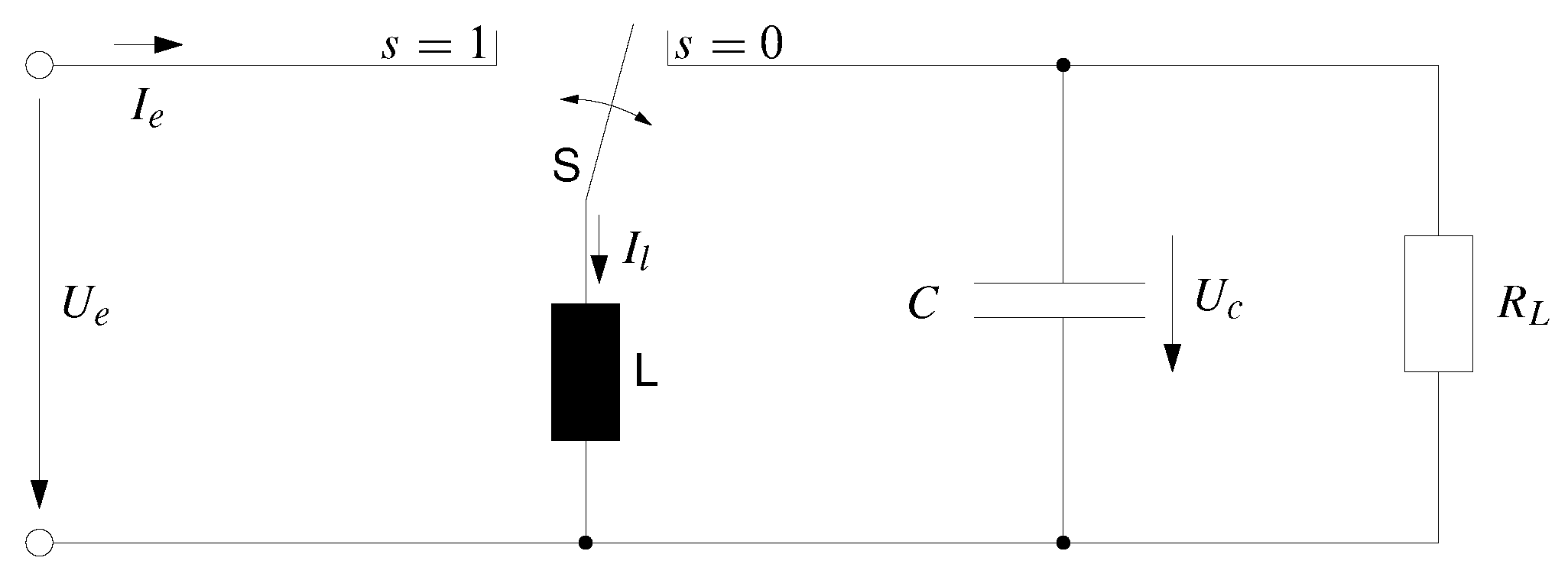
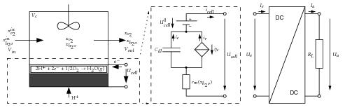
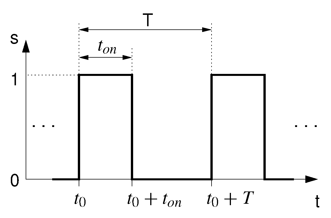
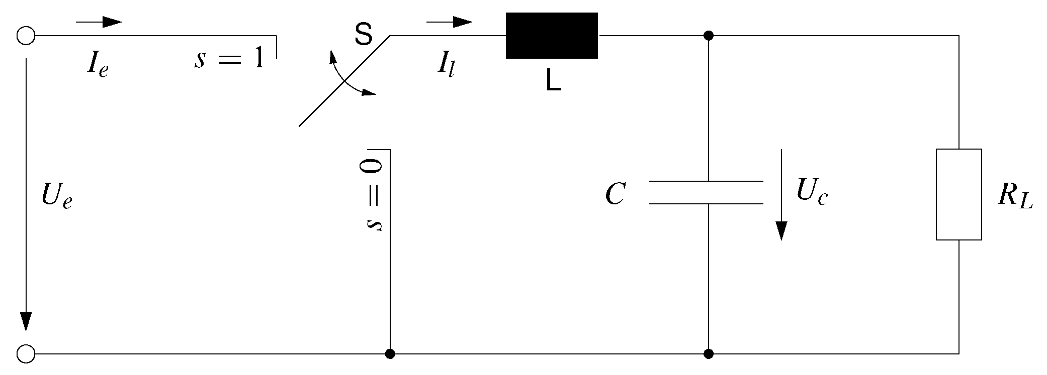
4.1. PEMFC and Boost-converter
In this section the coupling between the PEMFC and the boost converter is examined.
Effect of the converter ripple upon the PEMFC
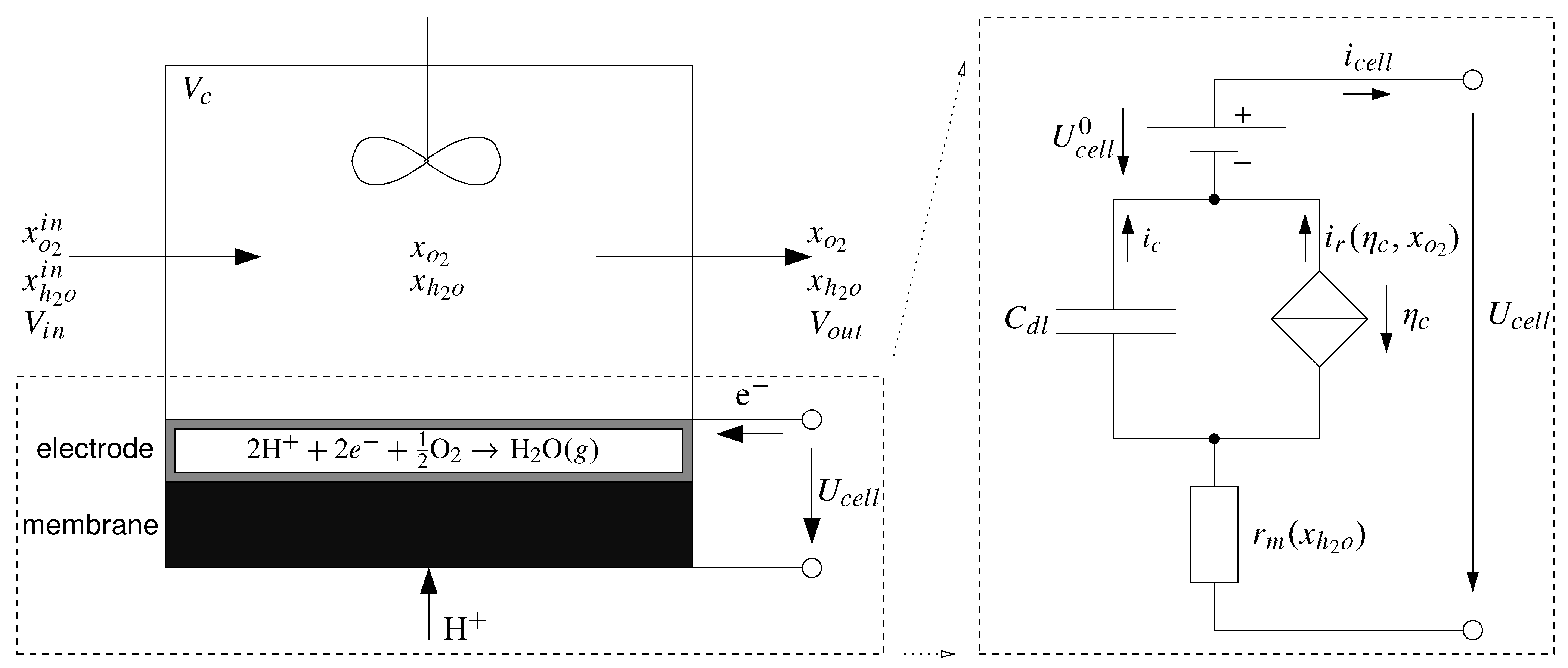
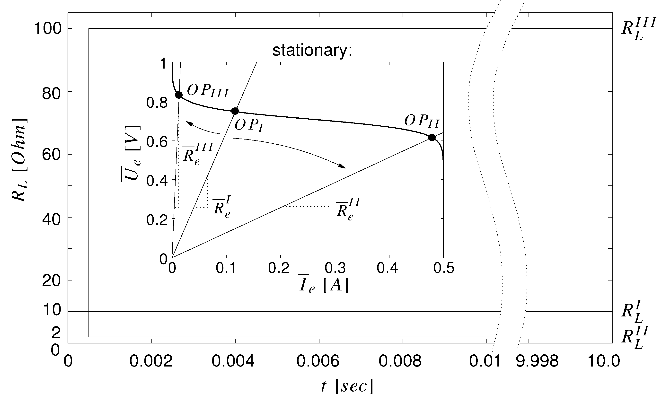
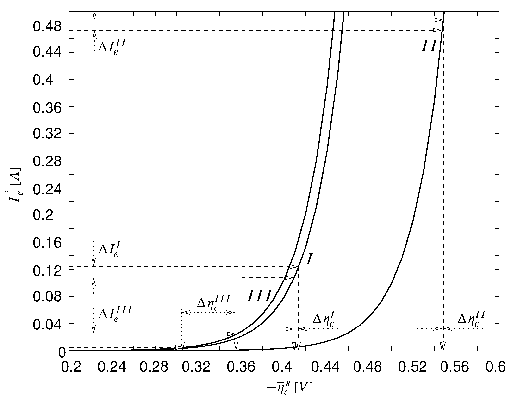
In a first step the effect of the converter ripple upon the PEMFC is shown. For this purpose the PEMFC (Eqns. (1-3)) and the boost converter model (Eqns. (6,7)) are coupled via Eqn. (13) and form a system of switched differential equations. This system is dynamically simulated using step changes of the load resistance
depicted in
Figure 7. The converter’s duty ratio
a is set to
and the other model parameters are kept constant at their nominal values. Three simulations
are performed with the same initial value
. In simulation
I the load resistance is kept constant at
whereas in simulations
and
the load is stepped to
and
respectively.
Figure 7.
Time plot of load resistance and stationary voltage-current profile of the PEM fuel cell with assigned operating points.
Figure 7.
Time plot of load resistance and stationary voltage-current profile of the PEM fuel cell with assigned operating points.
The simulation scenario can be further illustrated with the stationary voltage-current profile of the PEMFC together with the considered operating points
,
and
shown inside of
Figure 7. The operating points are determined by the load resistance
. A relationship between
and
can be derived from the averaged version of the boost converter model in Eqns. (6,7):
For the stationary operation of the converter one obtains:
and
. The average input resistance of the boost converter is given by
and with the dependency
one obtains from the previous statements
.
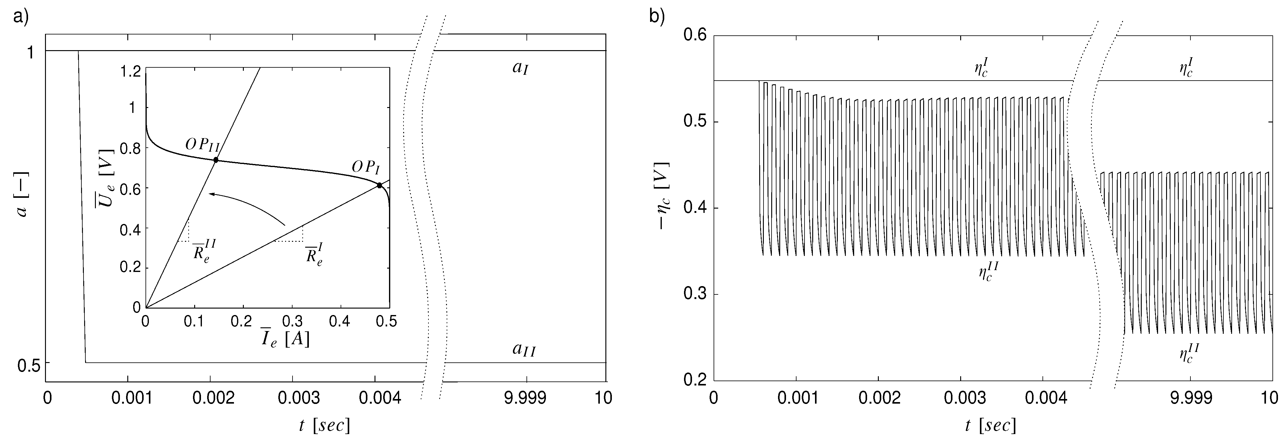
The simulation results are shown in
Figure 8 and
Figure 9. The diagrams are split into two parts. The first part shows the time plots from the simulation start to the settlement of the electrical transients of the coupled system. The second part shows stationary simulations after the transients for mass transport of oxygen and water vapor have settled. It can be seen, that during simulations
I and
no significant impact from the PEMFC to the boost converter or vice versa can be found. After the applied step the simulation settles and finally reaches a steady state. The oscillations of the quantities are small and can be neglected. In contrast, if simulation
is considered a clear interaction of PEMFC and converter can be observed. The overpotential
and the cell voltage
in
Figure 8 show relatively large oscillations compared to the cases
I,
. The oscillations are present immediately after the applied step and also at steady state. This is not the case for the converter input current
and the capacitor voltage
in
Figure 9. Both of them show only small oscillations in case
, similar to the simulation cases
I and
. The given interaction is therefore one-sided in direction from boost converter to PEMFC and is located at small cell currents in the activation polarization region of the fuel cell (
Figure 7).
The reason for this interaction can be found from the model equation of the overpotential in Eqn. (3). A linearization of this equation at an averaged and stationary operating point
of
Figure 8.
a) Step response of overpotential and b) cell (=converter input) voltage .
Figure 8.
a) Step response of overpotential and b) cell (=converter input) voltage .
Figure 9.
a) Step response of converter input (=inductor) current and b) capacitor (=converter output) voltage .
Figure 9.
a) Step response of converter input (=inductor) current and b) capacitor (=converter output) voltage .
the coupled system leads to
where
and
are the variations of the overpotential and the converter input current around the operating point respectively. It is assumed, that the variation of the oxygen content
due to the converter switching can be neglected. The variation
of the converter input current is considered as an input quantity in Eqn. (14), which is independent from
because of the observed one-sided interaction from converter to PEMFC. Equation (14) is therefore a linear ordinary differential equation of first order with constant coefficients whose transient behavior is determined by its time constant
τ. If the time constant
τ is small compared to the given time interval of the duty cycle
T then the variation
can approximately be calculated by
This relationship is determined from the Tafel kinetic in Eqn. (15) where
is the sensitivity of the overpotential
with respect to the cell current
. It can be seen, that the sensitivity increases with decreasing cell current. If the variation
does not change very much at different cell currents
, the change of variation
can approximately be determined by the changed sensitivity. This is the case for the three simulation experiments above. The oscillations
in the cell current (
Figure 9a) are nearly the same for all three simulation cases, but the average values are clearly different. For simulation case
the average cell current is the smallest resulting in the largest sensitivity of the three cases. The large oscillations in the overpotential for case
(
Figure 8a) are the consequence. In
Figure 10 the above statements are illustrated. The Tafel equation (15), the oscillation amplitudes of the cell current
(
Figure 9a) and the corresponding amplitudes of the overpotential
(
Figure 8a) are shown for the three simulation cases
I,
and
.
We have seen, that the reason for the large oscillation is a too small time constant τ with respect to the duty period T. From Eqn. (14) we can see, that the time constant τ is proportional to the double layer capacitance and (with Eqn. (16)) to the sensitivity . The sensitivity in simulation is the largest, so the double layer capacitance of the fuel cell is responsible for the small τ. Therefore, the oscillations in the activation polarization region of the PEMFC in are caused by an insufficient adaption of the double layer capacitance and the duty period T to each other.
Discussion of the effect
We have shown and explained in the previous section that the converter ripple introduces oscillations in the activation polarization region of the fuel cell. This statement is true for the used double layer capacitance
and duty period
T, but it is also in general valid as long as the ratio between
and
T is less or equal to the given one. This means for example, that we cannot increase
T in order to decrease switching losses in the boost converter, because this will result in larger oscillations in the fuel cell. This also means for example, that if the fuel cell owns a larger double layer capacitance
and we use the same duty period
T the oscillations will vanish. If we increase the duty period
T (and
Figure 10.
Tafel equation for simulation cases I, and .
Figure 10.
Tafel equation for simulation cases I, and .
the boost converter’s inductivity
L, capacitance
C to stay at the same ripple in the output voltage
) the oscillations will reoccur.
The impact of converter introduced oscillations in the overpotential is currently under research and up to now it is not clear, if they lead to cell degradation, as long as no reactant depletion appears [
12]. Anyway, in order to avoid oscillations in the fuel cell we have to take suitable measures which are presented in the following. For the above simulations we used a small double layer capacitance in the order of magnitude as in [
13,
14]. In other publications like in [
15,
16] a larger double layer capacitance in the PEMFC is observed. For the latter case, the oscillations in the fuel cell vanish for the given duty period and no further effort has to be taken to avoid them. In the first case there are two simple possibilities to avoid oscillations. The first is to decrease the duty period
T. This has a smaller variation
of the cell current and a larger impact of the time constant
τ within the time interval
T as a consequence, but can also lead to larger switching losses in the converter. The second alternative is to increase the double layer capacitance
of the PEMFC and therefore the time constant
τ. The first point can be achieved via the control of the boost converter. After the boost converter has been designed [
7] and the duty period
T has been adjusted to meet the boost converter’s requirements, a minimal cell current
has to be specified. This puts an upper bound on the sensitivity in Eqn. (16). If the double layer capacitance and all other necessary parameters are roughly known then the relevant time constant
can be estimated. If
oscillations are expected to appear if the fuel cell is operated in the activation polarization region. In order to avoid these oscillations the duty period
T can be decreased, e.g.
. The second possibility can be implemented for example by inserting a capacitor between PEMFC and boost converter. This leads to an increased double layer capacitance as is shown in
appendix B.
Overall behavior of the coupled system With the above suggestions the impact of the converter ripple can be suppressed and we can describe the connection between the PEMFC and the boost converter with averaged model equations and check the overall behavior of this coupled system for the occurrence of stationary multiplicities and oscillations.
At first, we consider the stationary operation of PEMFC and boost converter. Therefore, the stationary and averaged relationship in
Figure 6 for the boost converter is valid. Due to the coupling in Eqn. (13) the input resistance of the converter
serves as load resistance of the PEMFC
and forces a rheostatic operation of the cell. Moreover, the mapping between the converter’s input resistance
and the load resistance
is unique as is indicated in
Figure 6b. Therefore, no further stationary multiplicities are added by the coupling PEMFC and boost converter to the ones that are already present in a rheostatic operated PEM fuel cell [
17,
18,
19].
However, oscillations induced by the coupling are still possible. They appear if a Hopf bifurcation occurs due to the coupling. A Hopf bifurcation appears in a nonlinear system
if a pure imaginary pair of eigenvalues of the Jacobian matrix
, evaluated at the steady state
arises at the parameter
. Therefore, in order to search for the onset of oscillations, we have to check the Jacobian matrix of the coupled system. For this purpose we start with the following averaged model of PEMFC and boost converter:
It is derived by coupling Eqns. (
1-7) using Eqn. (13) and averaging, like in Eqn. (12), the resulting model over one duty cycle. For this purpose it is assumed that the states
are approximately constant during one duty cycle. This is a valid assumption due to the negligible impact of the converter ripple.
The above system of equations includes averaged model equations for oxygen and water transport (Eqn. (17,18)). This mass transport typically shows transient times in the order of magnitude of seconds while the resonant behavior of the converter is in the order of magnitude of milli seconds and smaller. Due to this we consider the mass transport Eqns. (17,18) as static and use only the equations (19-21) to search for the appearance of a Hopf bifurcation.
The first step in order to detect a Hopf bifurcation is the calculation of the Jacobian matrix. If we calculate the Jacobian matrix of equations (19-21) at the steady state
we get
The duty ratio
of the boost converter is typically between
and therefore, the coefficients
of
are always greater than zero. In the next step we have to check the location of the eigenvalues of the Jacobian matrix
. The eigenvalues of
are the roots of the characteristic polynomial
which is given by
The location of the roots of
can be determined with the criterion of LIÉNARD-CHIPART [
20]. The polynomial has only roots with negative real parts if the following necessary and sufficient conditions are fulfilled:
and
. The first two conditions are fulfilled through Eqns. (24,26), because the coefficients
,
and
of the polynomial are always positive. The third condition is also fulfilled, because of
Therefore, the characteristic polynomial
(Jacobian matrix
) has always roots (eigenvalues) with negative real parts and because of this the connection between a PEMFC and a boost converter cannot lead to a Hopf bifurcation in the coupled PEMFC - boost converter system.
4.2. PEMFC and Buck-converter
In this section the coupling between the PEMFC and the buck converter is examined.
Effect of the converter ripple upon the PEMFC In the first step we consider the effect of the buck converter ripple upon the fuel cell. For this purpose we couple the PEMFC (Eqns. (
1-3)) and the buck converter model (Eqns. (8,9)) with Eqn. (13) and apply step changes of the duty ratio
a (
Figure 11a) to this system. The load resistance
is chosen such that the fuel cell is operated close to the maximum power point. The other model parameters are at their nominal values. Two simulations
I,
are carried out. In simulation
I the duty ratio
a is kept constant at
and in
the duty ratio is stepped to
. The simulation scenario can be further illustrated by the stationary voltage current profile of the fuel cell and the considered operating points
and
. It is shown inside of
Figure 11a. The operating points are determined by the buck converter’s input resistance
via the converter’s duty ratio
a from the following dependency
with
. This relationship can be derived in an analogous manner from an averaged and stationary version of the buck converter model like it was done for the boost converter in
section 4.1.
The simulation results are shown in
Figure 11b and
Figure 12. The diagrams are split into two parts. As in
section 4.1, the first part shows the fast dynamics due to electrical effects, the second part shows the long term behavior, after the transients of the mass balances have settled. In simulation
I the duty ratio is equal to
. This means that the switch
S of the buck converter is always in position
and no oscillations occur. In contrast, if simulation
is considered, relative large oscillations in the overpotential
(
Figure 11b), cell current
(
Figure 12a) and the cell voltage
(
Figure 12b) are appearing. The large oscillations are present immediately after the applied step and also at the steady state. This is not the case for the inductor current
(
Figure 12a) and the capacitor voltage
Figure 11.
a) Time plot of duty ratio a and (inside) the stationary voltage-current profile of the fuel cell with considered operating points. In b) the step response of the overpotential is shown.
Figure 11.
a) Time plot of duty ratio a and (inside) the stationary voltage-current profile of the fuel cell with considered operating points. In b) the step response of the overpotential is shown.
Figure 12.
a) Step response of inductor current and cell (=converter input) current . In b) the step responses of cell (=converter input) voltage and capacitor (=converter output) voltage are shown.
Figure 12.
a) Step response of inductor current and cell (=converter input) current . In b) the step responses of cell (=converter input) voltage and capacitor (=converter output) voltage are shown.
(
Figure 12b) of the converter. Both of them show only small oscillations. The given interaction is therefore one-sided in direction from the buck converter to the PEMFC. The reason for the relatively large oscillations in the PEMFC is due to the presence of the switching function
s in the coupling of fuel cell and buck converter:
. This leads to a switched ODE for the overpotential:
and causes the large oscillations in the overpotential and in the cell voltage.
Discussion of the effect
The above equation can be used to further discuss the oscillation amplitudes of the overpotential. With the above observation that the interaction is one-sided from buck converter to the fuel cell and the assumptions that the changes in the inductor current
and the oxygen content
are small over one duty period
T and can be approximately described by their average values
and
, the following formula can be derived for the stationary oscillation amplitudes
of the overpotential:
The derivation of this equation is given in
Appendix C. The equation can be used to further investigate the oscillations in the fuel cell.
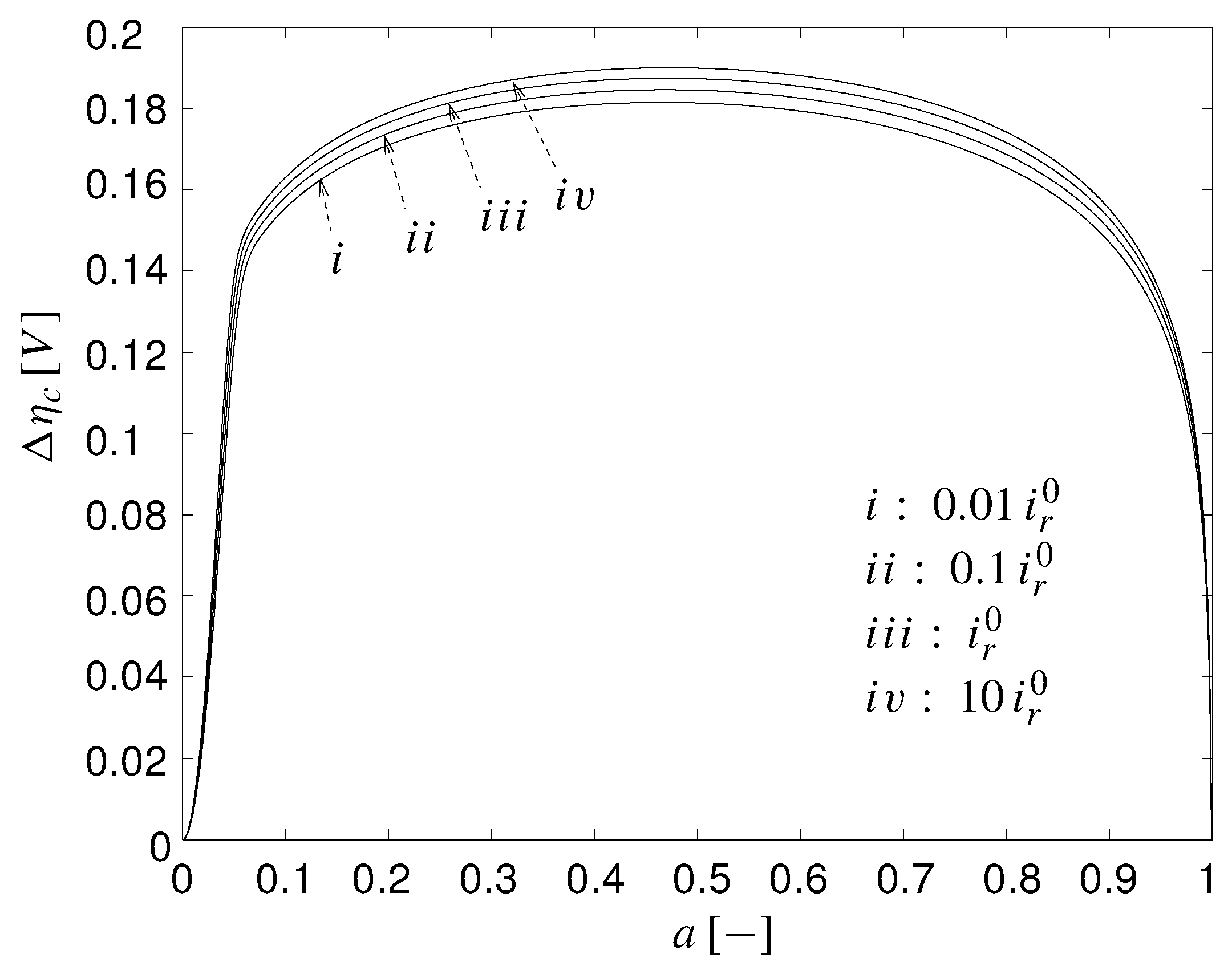
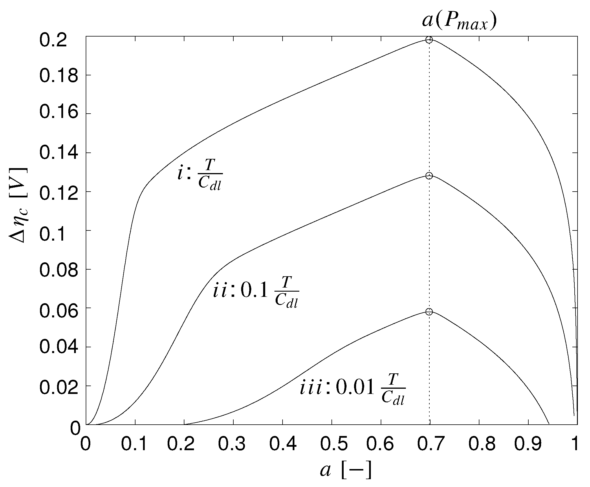
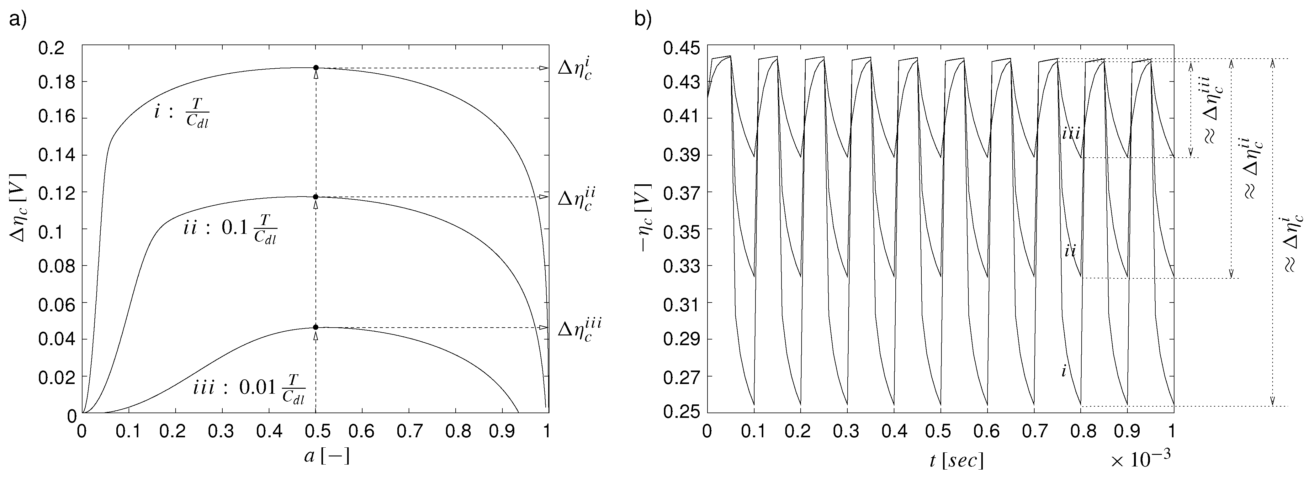
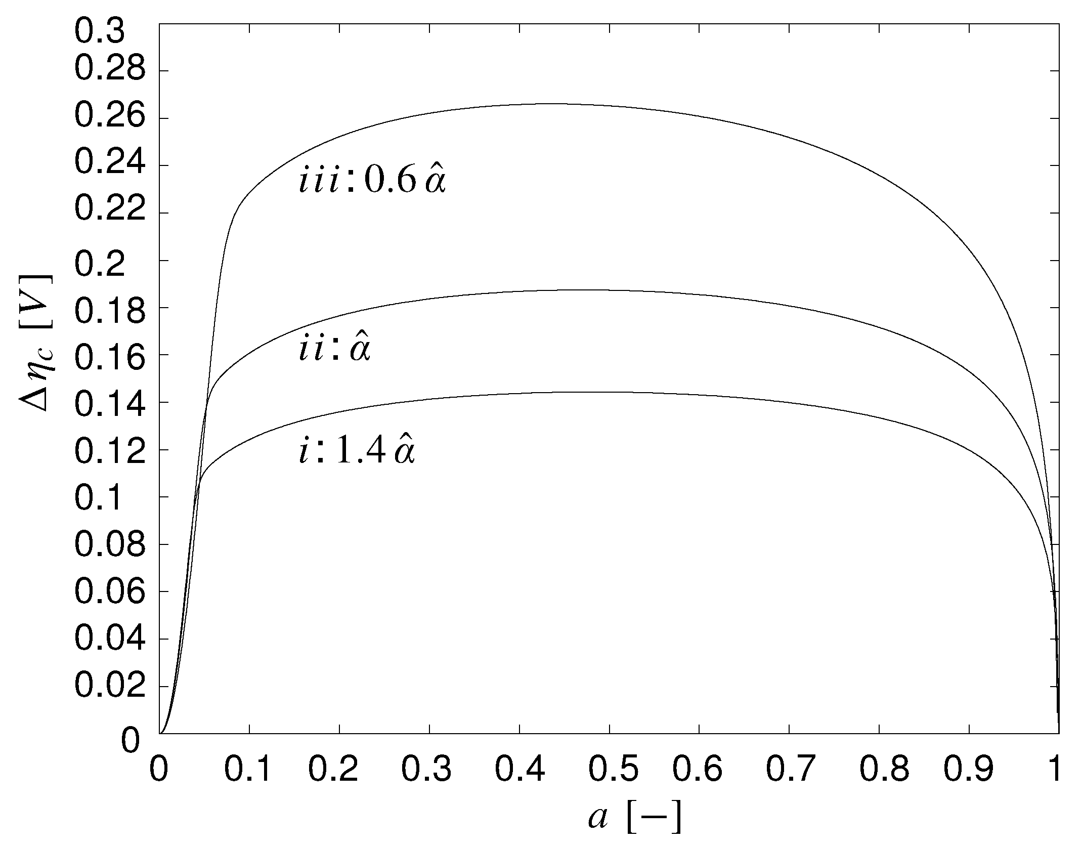
Figure 13a shows the oscillation amplitudes
calculated with Eqn. (29) at different duty ratios
a. The ratio of duty period and double layer capacitance
is used as parameter and the other quantities remain constant at their nominal values. It can be seen, that a
Figure 13.
a) Stationary oscillation amplitudes of the overpotential with respect to the buck converter’s duty ratio a at different ratios of duty period and double layer capacitance and b) stationary simulations of the overpotential for the cases i to at a duty ratio .
Figure 13.
a) Stationary oscillation amplitudes of the overpotential with respect to the buck converter’s duty ratio a at different ratios of duty period and double layer capacitance and b) stationary simulations of the overpotential for the cases i to at a duty ratio .
decreasing ratio of
leads to smaller oscillations in the overpotential and vice versa. Therefore, in order to reduce oscillations in the fuel cell either the duty period
T of the buck converter has to be decreased or the double layer capacitance
of the PEMFC has to be increased or both things have to be done. As was discussed in
section 4.1, this can be achieved either by adjusting the switching period of the converter or by adding a capacitor. In
Figure 13b an increased double layer capacitance is used. Stationary simulation results of the overpotential
for the coupled PEMFC and buck converter model at a duty ratio
are shown. The duty period
T is held constant and the double layer capacitance is increased from its nominal value in case
i to
in case
and
in case
. One can see, that the oscillation amplitudes of the overpotential decrease (
) as it is predicted in
Figure 13a.
The oscillations in the overpotential due to the coupling of PEMFC and buck converter may also be used to estimate parameters of the fuel cell. This may be useful for monitoring or control purposes of the PEMFC. Rather expensive to obtain are the parameters describing the reaction kinetics of the fuel cell. Their identification is usually done in experiments using the impedance spectroscopy, the current interrupt technique [
21] and the electrochemical parameter identification [
22]. Equation (29) may also be used for this purpose. For an estimation of the fuel cell’s reaction kinetics the exchange current density together with the cell’s oxygen content
, the exponent in the Tafel equation
and the double layer capacitance
have to be determined. If we want to identify these parameters from Eqn. (29) we need to know the average inductor current
and the oscillation amplitude
of the overpotential while the other quantities are rather well known. The quantity
can be obtained by measuring and averaging the inductor current. The oscillation amplitude
can be obtained by measuring the oscillation amplitude
of the cell voltage. If the fuel cell is well humidified the ohmic and concentration losses are negligible and we have
.
If
and
are known we have to analyze the sensitivity of these measurements with respect to the unknown parameters in Eqn. (29) to get an indication about the quality of the obtainable estimation results. For the double layer capacitance
we can use
Figure 13 for this purpose. If we define the changes of the oscillation amplitude
with respect to changes in
at some fixed duty ratio
a as sensitivity
we can see from
Figure 13a that this sensitivity should be large enough for all duty ratios to get acceptable estimation results for
. The sensitivity with respect to the exchange current density
is analyzed in
Figure 14. If we consider the changes of the oscillation amplitude
with respect to the changes in
at some duty ratio
a as sensitivity
it can be seen, that this sensitivity is rather small. Therefore, we cannot expect to get acceptable estimation results for
from Eqn. (29).
Finally, in
Figure 15 the sensitivity with regard to the parameter
(Eqn. (4)) is examined. If we consider the changes of the stationary oscillation amplitude
with respect to the changes in
at a duty ratio
a as sensitivity
it can be seen from
Figure 15, that this sensitivity should be large enough for duty ratios between
and
to get acceptable estimation results for the parameter
. The estimation results for
can be used to determine the transfer coefficient
α from Eqn. (4), since the relative change of
in
corresponds to a relative change of
in the transfer coefficient. To determine
α from Eqn. (4) the cell temperature Θ has to be roughly known, e.g. from measurements. In summary, the sensitivity analysis reveals that acceptable estimation results can be expected for the double layer capacitance
and the parameter
. The exchange current density cannot be estimated due to its small sensitivity. It should be noted, that due to this fact the precise value of the exchange current density as well as the precise value of the oxygen content in the cathodic catalyst is not necessary
Figure 14.
Stationary oscillation amplitudes of the overpotential with respect to the buck converter’s duty ratio a at different exchange current densities .
Figure 14.
Stationary oscillation amplitudes of the overpotential with respect to the buck converter’s duty ratio a at different exchange current densities .
Figure 15.
Stationary oscillation amplitudes of the overpotential with respect to the buck converter’s duty ratio a at different values of .
Figure 15.
Stationary oscillation amplitudes of the overpotential with respect to the buck converter’s duty ratio a at different values of .
for an estimation of
and
. The estimation requires the measurement of the average inductor current and the oscillation amplitude of the cell voltage at a highly humidified fuel cell. It should not be carried out at too small oscillation amplitudes
to reduce the impact of the neglected inductor current ripple in Eqn. (29).
Overall behavior of the coupled system If we suppress the oscillations in the fuel cell and neglect the impact of the buck converter ripple, we can describe and analyze the coupling between the PEMFC and the buck converter with averaged model equations in order to check the overall behavior of the coupling for the appearance of stationary multiplicities and oscillations.
First of all, the stationary operation of PEMFC and buck converter is considered. Therefore, the stationary and averaged relationship in
Figure 6 for the buck converter is valid. Like in the case of the PEMFC and the boost converter, the same reasoning is true and therefore the coupling between PEMFC and buck converter cannot introduce further stationary multiplicities as are already present in the PEMFC. However, oscillations induced by the coupling are still possible. In order to analyze the onset of oscillations we start with the following averaged model of PEMFC and buck converter:
It is derived by coupling the model equations of the PEMFC (
1-3) and the buck converter (8,9) via Eqn. (13) and averaging the resulting equations over one duty cycle. This is done in the same way as for the boost converter above. Like there, we consider the equations for the mass transport Equation (30,31) as static and use only the averaged model equations (32-34). The Jacobian matrix of these equations evaluated at the steady state
is given by
The duty ratio for a buck converter is typically between
. With this, the coefficients
in
are always positive and therefore the same reasoning as in the previous analysis of PEMFC and boost converter is true: The connection between a PEMFC and a buck converter cannot introduce a Hopf bifurcation in the coupled PEMFC - buck converter system.
4.3. PEMFC and Buck-Boost-Converter
In this section the coupling between the PEMFC and the buck-boost converter is examined.
Effect of the converter ripple upon the PEMFC In a first step the effect of the converter ripple upon the fuel cell is considered by analyzing the coupled system of switched differential equations made up from the PEMFC (Eqns. (
1-3)) and the switched buck-boost converter model (Eqns. (10,11)). The analysis reveals that the buck-boost converter introduces oscillations in the fuel cell in the same way as the buck converter. As in this previous case, the reason is due to the presence of the switching function
s in the coupling of the fuel cell and the buck-boost converter:
. This leads to the same switched ODE for the overpotential (28) and causes the oscillations in the fuel cell.
Discussion of the effect The formula for the oscillation amplitude
in Eqn. (29) can also be used to describe the stationary oscillations introduced by a buck-boost converter.
Figure 16 shows the oscillation amplitude of the overpotential calculated with this formula at different duty ratios. The ratio of the duty period and the double layer capacitance
is used as parameter. The load resistance
is set to
while the other quantities remain constant at their nominal values. It can be seen from
Figure 16,
Figure 16.
Stationary oscillation amplitudes of the overpotential with respect to the buck-boost converter’s duty ratio a at different ratios of duty period and double layer capacitance . The quantity denotes the duty ratio at the maximal cell power .
Figure 16.
Stationary oscillation amplitudes of the overpotential with respect to the buck-boost converter’s duty ratio a at different ratios of duty period and double layer capacitance . The quantity denotes the duty ratio at the maximal cell power .
that a decreasing ratio of
leads to smaller oscillations in the overpotential and vice versa. This is the same qualitative behavior as in the case of the buck converter in
Section 4.2. Therefore, the same possibilities to reduce the oscillations are applicable.
The connection between the PEMFC and the buck-boost converter can also be used to estimate parameters of the fuel cell. We can use Eqn. (29) for this purpose again. In detail, the double layer capacitance
and the exponent of the Tafel kinetics
can be estimated. In the case of the double layer capacitance this can be seen from
Figure 16. The sensitivity
of the oscillation amplitude with respect to the double layer capacitance should be large enough to get acceptable estimation results for
. In the case of the parameter
we can use
Figure 17. We see, that the sensitivity
of the oscillation amplitude
with respect to
should be large enough to get acceptable estimation results for
too.
Figure 17.
Stationary oscillation amplitudes of the overpotential with respect to the buck-boost converter’s duty ratio a at different values of . The quantity denotes the duty ratio at the maximal cell power .
Figure 17.
Stationary oscillation amplitudes of the overpotential with respect to the buck-boost converter’s duty ratio a at different values of . The quantity denotes the duty ratio at the maximal cell power .
Overall behavior of the coupled system If we reduce the oscillations and are able to neglect the impact of the converter ripple we can finally analyze the overall behavior of the coupled PEMFC and buck-boost converter with averaged model equations.
First of all, the stationary operation of PEMFC and buck-boost converter is considered. Like for the previous two converters the same reasoning is true and therefore the coupling between PEMFC and buck-boost converter cannot introduce further stationary multiplicities as are already present in the PEMFC. However, oscillations are still possible and their appearance has to be analyzed. This is done by coupling and averaging the model equations of the PEMFC (
1-3) and the buck-boost converter (10,11) in the same way like in the previous two cases. We obtain the same mass transport equations for oxygen and water vapor like in the case of the buck converter (Eqns. (30,31)). Like there, we assume them as static and use only the model equations for the overpotential and the buck-boost converter’s inductor current and capacitor voltage:
If we calculate the Jacobian matrix of the above system at the steady state
we get
The duty ratio of the buck-boost converter is typically between
. With this, the coefficients
of
are always positive and the coefficients
,
are always negative. If we calculate the characteristic polynomial of
we get the equations (23-26) with negative quantities
and
. Despite this difference, the coefficients
,
,
of the characteristic polynomial and the condition
are still positive due to the fact that only the positive product
enters the determining equations (24-27). Therefore, the same conclusion as in the case of the PEMFC and the boost converter applys: The connection of a PEMFC and a buck-boost converter cannot induce a Hopf bifurcation in the coupled system.

