
Hierarchical Control and Economic Optimization of Microgrids Considering the Randomness of Power Generation and Load Demand
College of Information Science and Technology, Donghua University, Shanghai 201620, China
*
Author to whom correspondence should be addressed.
Energies 2023, 16(14), 5503; https://doi.org/10.3390/en16145503
Submission received: 29 June 2023
/
Revised: 16 July 2023
/
Accepted: 18 July 2023
/
Published: 20 July 2023
(This article belongs to the Section C: Energy Economics and Policy)
Abstract
:Hierarchical control has emerged as the main method for controlling hybrid microgrids. This paper presents a model of a hybrid microgrid that comprises both AC and DC subgrids, followed by the design of a three-layered control method. An economic objective function is then constructed to account for the uncertainty of power generation and load demand, and the optimal power guidance value is determined using the particle swarm optimization algorithm. The optimized power output is subsequently used to guide the tertiary control in the microgrid, mitigating potential safety and stability issues. Finally, the performance of each control layer is compared under dynamic changes in AC and DC loads, as well as stochastic variations in power generation and load consumption. Simulation results demonstrate that the hybrid microgrid can function stably, ensuring reliable and cost-effective AC and DC bus voltage supply despite the randomness of power generation and load demand.
1. Introduction
Developing a smart grid involves addressing the challenges of large-scale distributed energy generation and replacing passive distribution networks with active ones. Microgrids can be a viable solution, as they integrate distributed generations (DGs), loads, energy storage devices, power electronic converters, and protection devices into a single system. Integrating sources of alternative energy, including wind and photovoltaic generators, requires solutions for optimizing energy flow scheduling. This will improve the predictability, controllability, and dispatchability of new energy generation. A mixed AC and DC microgrid can be used to solve the hierarchical control problem and ensure the stability and reliability of the microgrid operation and energy supply [1].
For complex microgrid systems, hierarchical control is the main approach [2,3]. For a hybrid AC/DC microgrid, the hierarchical control is divided into three levels: primary, secondary, and tertiary control. Each level has distinct responsibilities that complement one another. The primary control handles power allocation, local frequency, and voltage stability. The secondary control corrects operational status deviations that come from the primary control, while the tertiary control handles the optimization of power dispatching. The first two layers of control are responsible for the system’s overall stability, and scheduling optimization is performed based on this. This paper employs this concept to develop a layered control system.
Optimizing the scheduling of microgrids is a complicated optimization problem that requires balancing electricity generation and load demand to ensure the safety and stability of microgrids [4,5]. In order to achieve this, optimization scheduling needs to consider not only the economic cost of power generation but also the reliability of the power supply from distributed power sources. There are various methods and scheduling strategies proposed in existing research related to this issue. For example, in [6], a novel power scheduling approach is proposed for economic dispatch in microgrids with high levels of renewable energy. The approach minimizes net cost and is solved in a distributed fashion using local controllers. In [7], a new battery operation cost model is proposed to incorporate renewable resource uncertainties into a unit commitment problem and enable efficient and economical energy storage coordination. In [8], a two-stage optimization approach for scheduling energy generation in a microgrid with multiple generators and storage systems is proposed, minimizing operating costs and handling uncertainties. In [9], an energy management system is implemented for campus microgrids to reduce operational costs, resulting in a reduction in grid electricity costs. While existing microgrid optimization methods perform well, they are not highly integrated with microgrid hierarchical control, and some of them do not address the control problems at the power converter level. Specifically, there is little attention paid to how the optimized scheduling strategies generated can be applied at the device level to achieve a good combination of optimization and control.
Additionally, there have been studies targeting the multi-objective model for economic and environmental optimization, as well as the stability of microgrid scheduling operations with power units that also have specific functions in a hierarchical type, such as electric vehicle [10,11,12], energy storage [13,14,15], and multi-type power generation [16,17,18]. However, there is a lack of research on the economic optimization problem in the context of stochasticity brought by power generation and load demand, particularly in relation to primary and secondary controls and how to reflect them in tertiary control. This paper proposes a microgrid model consisting of wind power, photovoltaic, and dynamic loads and uses the particle swarm optimization algorithm (PSO) to optimize microgrid control, thereby further improving their performance and efficiency [19].
Given the existing problems mentioned above, this paper aims to achieve a stable power supply, conserve energy, and reduce emissions for the microgrid. The approach used is a hierarchical control-based hybrid microgrid collaborative control approach. A scenario is established to address uncertainties in microgrid optimization problems. The PSO algorithm is used to optimize the model’s objective function and ensure load power consumption reliability while fully utilizing power generation equipment. Renewable energy sources are then utilized for the tertiary control of the microgrid, improving power supply quality, reducing energy consumption, and achieving optimal operation. The paper presents the following main contributions:
- A hierarchical control approach is utilized for the collaborative control of an AC/DC hybrid microgrid, which includes primary and secondary control. This approach ensures a stable power supply for the microgrid.
- To optimize uncertain system scenarios resulting from the randomness of power generation and load demand in microgrid systems, the PSO algorithm is utilized. The algorithm generates the optimal operating cost and output power of the system, thereby achieving scheduling optimization of microgrid systems.
- A tertiary control of the microgrid system is proposed based on the optimal power guidance that considers the randomness of power generation and load demand. This control achieves a more stable output with smaller fluctuations in system frequency and bus voltage while also taking economic considerations into account.
Specifically, the innovation of this paper is the close integration of economic optimization and stable power supply of the bus in a microgrid system based on a three-level hierarchical control structure. This is different from the existing literature, which separates the two areas of research. Furthermore, the guidance power value that is produced through economic optimization gives precise configurations for tertiary control and distinct indications for underlying controls.
The microgrid structure analyzed in this paper is shown in Figure 1. Currently, AC microgrids are the primary type, linked to the main grid via an electrical switch that enables the transition from islanded to grid-connected mode. A DC subgrid connects photovoltaic power sources, converters, and loads to the AC subgrid via a DC bus, utilizing bidirectional converters for interconnections between the two subgrids [20,21]. The AC subgrid has the capacity to accommodate wind power sources through converters and an AC bus. The hybrid microgrid is managed as an AC grid to facilitate reliability and attempt to combine the advantages of both types for the main grid.
This paper includes five sections. Section 2 provides basic hierarchical control and power generation of the microgrid used in this paper. Section 3 introduces scenario modeling and the PSO algorithm for optimizing the objective function and identifies the optimal power generation. Section 4 conducts the simulation and analyzes the results. Lastly, Section 5 summarizes the entire study.
2. Hierarchical Control of Hybrid Microgrid
2.1. Primary Control
Primary control focuses on the stability of local control and the drive signal of power converters. AC subgrid control mainly focuses on the AC-bus frequency and voltage amplitude, while DC subgrid control mainly focuses on the DC voltage amplitude. Droop control is a common method for parallel AC/DC interface DGs, which can autonomously share load power. Specifically, the active and reactive power of AC DGs are controlled in the AC subgrid, while the output voltage of DC DGs is controlled in the DC subgrid. In order to obtain appropriate AC frequency and voltage amplitude ω and E, the measured active and reactive power values P and Q should compare with the reference values P* and Q* respectively, generated by droop equation [22]:
where ω* and E* are references of ω and E, and m and n represent the droop slope or coefficient.
The settings of m and n are as follows:
where the maximum deviations of frequency and voltage limits are represented as Δω and ΔV, respectively, while Pmax and Qmax represent the maximum values of inverter output active and reactive power.
DC subgrids have simpler voltage droop control compared to AC microgrids due to the absence of regulation of reactive power and frequency. The equation for droop control in DC subgrids is [23]:
where Vmax is the maximum available transmission voltage when the light load connects; Rd is the droop coefficient:
where Vmin is the minimum available output voltage under full load conditions, and Imax is the maximum available output current.
2.2. Secondary Control
To overcome primary control deviations, secondary control methods are typically used to correct the deviations and restore them to their rated values. This study adopts a secondary controller for both AC and DC subgrids that measures frequency deviation and voltage deviation in a timely manner and then sends generated compensations to all DGs in the AC subgrids to restore frequency and voltage amplitude. This is achieved through the following formulas:
where the control coefficients Kpω, Kiω, KpE, and KiE are used for compensators in secondary control. As for the DC grid, since the frequency is not considered, compensating the voltage is sufficient to maintain the stability of the DC bus voltage and restore it to its rated value by using [24]:
The AC subgrid has the following equations to form secondary layer:
The DC subgrid is comprised of the following equations that form the secondary layer:
The connection between primary and secondary controls is that the primary control is decreasing in trend, and sometimes, the operating frequency drops below the rated value, which is not practical. To resolve this issue, we suggest raising the primary droop curve to an optimal level to bring the system back to its rated value under the current load. Utilizing these controls helps maintain the system at its rated value.
2.3. Tertiary Control
As the number of hierarchical control layers in microgrids increases, response speed slows. Power conversion allows for the real-time regulation of microgrids, but tertiary control does not due to its longer update cycle. Instead, tertiary control optimizes power flow distribution while considering economic principles and provides reference values for each microgrid unit [25]. Tertiary control involves managing the relationship between the microgrid and the main grid, as well as between different microgrids and subsystems within the microgrid. It mainly focuses on energy management, scheduling, and designing microgrid systems for economic benefits while ensuring stable operation. This paper seeks to enhance the effectiveness of microgrid systems by using mathematical optimization to calculate the best output power values for each distributed power source. The focus is on optimizing internal generation and load demand. These values are used to generate scheduling instructions sent to the secondary control. The next section will provide a detailed explanation of creating scheduling instructions for power references in AC subgrids.
The tertiary control process of the microgrid mainly compares the measured values of the power PG and QG of the static bypass switch with the reference power and and generates a difference. Then, the microgrid is controlled and regulated using the following formulas [2]:
where the control parameters of the PI controllers are represented by Kpp, Kip, KpQ, and KiQ. If and go beyond the limit, they will saturate. Grid synchronization and connection can start if they match the main grid.
3. Optimization of Microgrid System
3.1. Dynamic Optimization Modeling
The two main themes of microgrid control and optimization are stable power supply and optimized scheduling. Stable power supply focuses on frequency and voltage control, with a concentration on primary and secondary control levels. On the other hand, optimized scheduling’s optimization behavior is more reflected in the tertiary control level with a longer time update span. Currently, there are many studies on separating the two themes, but knowledge of how to achieve their common goals is still insufficient in the current research. Stable power supply and optimized scheduling are closely related and crucial for microgrid stability. Real-time monitoring and load adjustment maintain a stable power supply, reduce energy consumption, and enhance energy efficiency. Optimized scheduling involves reasonable energy scheduling and load management, which further enhance energy efficiency and economic benefits. However, fluctuations in new energy generation and user demand can increase operating costs and management complexity, lower energy efficiency, and result in load fluctuations, affecting main grids and microgrids.
For the simulation of output power uncertainty from new energy sources like photovoltaic and wind power in microgrids and the uncertainty of load demand changes within the system, uncertainty modeling is required. In this section, a scenario-based model is selected to simulate the uncertainty scenarios of load demand, wind power, and photovoltaic generation.
Wind power generation is the most important way to utilize wind energy by converting it into clean and efficient electrical energy. The probability distribution of wind speed is an important indicator to evaluate the status of wind energy resources, and there is a certain causal relationship between the probability distribution of wind speed and the output power of wind turbines. Different probability distributions of wind speed will have different effects on wind turbines’ output power.
Wind speed at different locations and times affect output wind powers. The probability density function of wind speed follows the Weibull distribution as the following formula [26]:
where v is the actual wind speed at the current time, and λ0 and k are parameters of the distribution function. k represents the shape coefficient of the distribution, and the different distribution curves are linearly related to this parameter, which is taken as two here. λ0 is the scale parameter.
The relationship between wind output power and speed is derived from Formula (16) as wind power output:
where PN is the rated wind turbine power, and vI, vT and vN are the cut-in, cut-out and rated wind speeds, respectively.
To calculate the expected output power of the photovoltaic power generation system, Markov models or beta distributions can be used to convert the distribution of sunlight intensity into the distribution of photovoltaic output power. The output power of photovoltaic cells in microgrids is directly related to the intensity of light, which follows a beta distribution, denoted by
where s is the light intensity at the current time, α0 and β0 represent the two coefficients of the beta fraction, and a and b represent the range of light intensity changes during a certain period.
Formula (18) can be derived to calculate the output power of photovoltaics:
where μ is the solar radiation intensity, SP is the panel area, ηP is the energy conversion efficiency, ηmax is the maximum power point tracking efficiency of the photovoltaic panel, and θ (usually taken as 45°) represents the tilt angle of the photovoltaic panel.
Probability distributions for the uncertainty of loads usually follow the normal distribution or Poisson distribution. The normal distribution is suitable for load changes in large systems, while the Poisson distribution is suitable for load changes in small systems. In addition, there are other distributions applicable to specific load change patterns, such as the exponential distribution applicable to some special load change scenarios. The command PoissonDistribution within MATLAB is used to model uncertain load demands. As this technology is widely used and understood within the software, it is omitted here. For those who are interested, further details can be found in the relevant manual.
3.2. Scenario Generation and Reduction
Simulating the output power of above-mentioned new energy sources in a simulated microgrid, this paper chooses a scenario-based model to simulate the demand uncertainty and the uncertainty scenarios of wind and photovoltaic power. The scenario generation and reduction process consist of the following two steps [27].
(1) Scenario generation: Assuming that the load demand, wind, and photovoltaic power generations in this problem are unknown. To simulate uncertainty, the forecast errors related to the load demand, wind power generation, and photovoltaic power generation are taken as known probability density functions. They are obtained as follows:
where PW,t,s, PPV,t,s and PL,t,s are the measured output power values of the wind turbine unit, photovoltaic unit, and load demand in scenario s at time t. , , and are the predicted values of the wind power, photovoltaic output power, and load demand at time t. , , and are the prediction errors related to the sum of the output power of the load demand, wind turbine unit, and photovoltaic unit in scenario s at instant t. Ns is the total scenario amount.
To generate different scenarios, begin by comparing the cumulative probability of the intervals listed above with an unplanned number falls in [0, 1]. Next, select the interval that is not greater than this number as the first interval, and assign a value of 1 to the binary parameters associated with that interval. Each scenario is represented by a binary vector, with binary parameters for electrical load demand and wind power and photovoltaic power intervals, as illustrated in Equation (20).
where , , and are binary value of the load demand, wind and photovoltaic power generations in scenario s at time t. The probability calculation formula for each scenario is as follows:
where the occurrence probability of the scenario is the cumulative probability of the prediction error of the load demand of intervals i, j, and k of wind and photovoltaic power at time t extracted, denoted as αi,t, βj,t, and γk,t, respectively.
(2) Scenario reduction: Simulating uncertainty with a large number of scenarios results in a significant increase in the required computation time and memory. To address these issues, after using scenario generation technology for scenario generation, reduce the scenario number to lower the computational load and memory requirements while ensuring the simulation effect. Similar to clustering algorithms, a large number of sample points can be divided into several categories, and each category can select a representative sample to describe as many statistical information as possible with as few scenarios as possible. This mainly simulates the uncertainty reduction of wind power, photovoltaic power generation, and load scenarios.
To circumvent the computational difficulties resulting from large-scale scenarios, a scenario reduction method based on probability distance rapid reduction algorithm is used to reduce the scenarios to 10 by probability partitioning [28]. After running, the reduced scenarios and generated scenarios are directly given, and the corresponding probabilities are provided and highly portable and applicable. Here, the fast-forward algorithm is used to cut down the scenario amount, which quickly identifies representative samples by using statistical methods and is suitable for scenarios that require rapid calculation [29]. Next is the procedure for the algorithm:
(a) Find the gap between each scenario ω via:
(b) Determine the average gap between one and the other scenarios. In this step, select the scenario ω1 with the smallest distance as the first selected scenario. AY and AN are, respectively, the selected and unselected scenario set; they are updated:
(c) Find the gap between each unselected scenario and selected scenario. Select the scenario with the minimized distance as the next selected scenario ωi, and update the unselected scenario set:
(d) Perform addition operations on probability using the following formula, where B(ω) is the set of unselected scenarios closest to ω.
3.3. Optimizing Function Creation and Problem Solving
Photovoltaic and wind power generation produce thermal energy during the reception of heat radiation and the friction of fan rotation, respectively. In order to prevent equipment damage and improve efficiency, this thermal energy is dissipated and collected through radiators or cooling devices. Large power stations typically have such thermal energy management systems. Therefore, microgrid systems that co-produce electrical and thermal energy can be optimized for the research below.
(1) Optimizing function creation: Here, we consider a microgrid system that can provide both heat and electricity and optimize the system economically while examining the impact of the optimization results on hierarchical control. We establish an objective function for the microgrid system based on economic costs, mainly including the operating costs of each generator unit, as shown in Equation (27).
where Ci () is the operating cost of a pure generator producing kW. The operating cost of a combined heat and power (CHP) generator producing kW of electricity and kWth of heat is denoted as Cj (, ). Ck () is defined as the operating cost of a pure heat generator producing kWth of heat. Np, Nc, and Nh are the total numbers of pure power, CHP, and pure heat generators, respectively. i, j, and k are the identifiers of the generators.
The cost function of each power-consuming unit is expressed as:
where , , , , and are the operating cost ratios of the ith pure power generator, and Pip represents the power output of the ith pure power generator. , , and are the coefficients used to calculate the operating cost of the kth pure heat generator, and represents the kth pure heat generator. , , , , , and are the operating cost coefficients of the jth CHP generator, and and are the power and heat outputs of the jth CHP generator.
In order to facilitate problem solving, some constraints with practical significance need to be taken into account [30]. The following factors have been considered:
(a) Power balance constraint
where Pd and Hd are the demand values of power and heat, and Ploss refers to the transmission loss of power systems. The power and heat energy from each unit meet the demand.
(b) Electric power output constraint
where and are the maximum and minimum power output limits of pure power generation units, and and are the upper and lower electric power output of CHP cogeneration units.
(c) Heat power output constraint
where and are the minimum and maximum heat power output of CHP cogeneration units, and and are used to represent the upper and lower limits of the output heat power of pure thermal power generation units.
(2) Problem solving: The optimization equation and constraints have been designed, and we need to solve the problem. To solve optimization problems in microgrid optimization, algorithms can have two types: mathematical analytical methods and intelligent algorithms. We choose the representative and mature PSO algorithm from the latter [31]. This algorithm is inspired by the group activities of birds and fish, and it can effectively solve various optimization problems. Each particle in the swarm represents a feasible solution, and they update their position and velocity based on their history and the history of the global optimal particle. The algorithm finds the fitness of each particle by evaluating the objective function and constraints. The algorithm will halt once a satisfactory solution has been found or the maximum number of iterations has been reached.
Here, the PSO algorithm is chosen because it is a well-established approach that has been proven to perform well in many problems. According to existing literature, PSO has received long-term attention because of its excellent global optimization ability and simple and efficient verification. Despite being a mature technology, it remains one of the preferred cost-effective solutions for many optimization problems. Additionally, there is a substantial body of recent literature that demonstrates its relevance and effectiveness in the context of microgrid applications [32,33,34,35,36].
The simplified process for the PSO usually includes the following steps:
- (a)
- Initialize the particle swarm’s position and velocity.
- (b)
- Determine the fitness value for every particle.
- (c)
- Update the global optimal solution.
- (d)
- Renew each particle’s velocity and position.
- (e)
- Repeat steps 2–4 until the condition is met.
- (f)
- Return the global optimal solution.
PSO can optimize microgrid load uncertainty and provide numerous benefits, such as accurate calculation results, intelligent scheduling, simplified operation, adaptability to varying scales and load requirements, and real-time load demand adjustments to improve reliability and stability.
The inertia weight (usually between 0 to 1) affects how fast particles move during the search process. A small value leads to slower but more stable search results, while a large value produces faster speed but less global optimal solution. To optimize the algorithm’s performance, an adaptive formula for the inertia weight can be used. It adjusts the value of w(t) at the tth iteration based on the upper and lower values of the inertia weight wmax and wmin and the maximum iteration number T of the algorithm.
This adaptive inertia weight strategy improves the algorithm’s efficiency, convergence speed, and search accuracy. Here, Figure 2 below shows the overall control block diagram. The diagram identifies three layers of hierarchical control and illustrates the relationship between the optimized power reference value of the microgrid and tertiary control. In our analysis, we focus solely on optimizing and analyzing the AC subgrid and tertiary control, as the current mainstream power grid is still optimized and scheduled in AC form, and most devices still operate on AC power. However, we recognize the need to study the optimization and control of both the DC and AC sides, which will be the subject of future work.
4. Simulation and Result Analysis
This section aims to verify the proposed hierarchical control and optimization discussed in this paper. First, it considers the performance of hierarchical control in hybrid microgrids. Then, it examines the scenario reduction under uncertain generation and consumption. Next, it conducts case studies and analyzes the results of microgrid economic optimization models. Finally, it performs microgrid control under optimal power guidance. Table 1 shows the configuration and control parameter selection of the microgrid used in this paper. In this paper, the simulation employs a discrete method with a time step of 10 ns for system state updates. From the beginning of the system initialization operation to the end of the entire 2.4-s simulation, it takes approximately 3 min. The simulation platform used is MATLAB R2022b, running on an Intel Core i7 CPU with 32 GB of RAM. A screenshot of the established simulation model and its control structure is shown in Figure 3. In the simulation of the CHP example, there are two AC-type DG systems and two DC-type DG systems. One of them is allocated to provide pure electricity, two are used for cogeneration, and the remaining one is used to provide pure heat.
4.1. Hybrid Microgrids’ Hierarchical Control Performance
A simulation model of a microgrid is established in MATLAB/Simulink to test the performance of an islanded hybrid microgrid system and its control strategy. The focus is on power distribution and voltage stability under variable quantitative load changes. The simulation compares the recovery performance of frequency and voltage amplitude under primary and secondary control in subgrids.
There have been changes in the load balance of the AC and DC subgrids. Specifically, the changes in system load include the following: at 0.4 s, a resistive load with a resistance value of 46 Ω was connected to the DC subgrid; at 0.6 s, a 20-kW load was added to the system and then disconnected from the AC subgrid again at 1.1 s.
Figure 4a,b show the control performance of the AC subgrid using hierarchical control. To achieve a truly authentic simulation effect, the curve changes from system initialization at 0 s are presented. It can be clearly seen that once a 20-kW load is linked to the AC subgrid under primary control at 0.6 s, the voltage and frequency quickly drop to 48.3 Hz and 299 V, respectively, and then maintain stability. When it is disconnected at 1.1 s to attain consistent state, the voltage and frequency quickly change to 48.83 Hz and 302.5 V, respectively, and again become stable. Initiating secondary control, the AC bus frequency reaches a stability at around 50 Hz, with frequency fluctuations of about 0.1 Hz. Except for the large controllable fluctuations during the initial system startup phase, the voltage stays at 310 V, with amplitude fluctuations of less than 1 V. This verifies the constructed hybrid microgrid model and demonstrates the restorative effect of the proposed hierarchical control technology on frequency and voltage deviations in the AC subgrid.
Next, Figure 5a,b describe the control performance of the DC subgrid. It can be clearly seen from the figures that although the voltage remains stable with the use of primary control, there will be a significant overshoot once the load changes, compared to the use of secondary control. In addition, the voltage fluctuation has an amplitude of approximately 10 V, while its steady-state value is around 998 V, which is lower than the rated value. With the addition of secondary control in the DC subgrid, the DC voltage stays at approximately 1000 V, with a maximum deviation of 5 V. This validates the effectiveness of the proposed control method for DC subgrid.
During load changes, the power distribution within the hybrid microgrid is shown in Figure 6a–c. The figure clearly illustrates that under the application of primary droop control, effective active power distribution is achieved in both the AC and DC subgrids. The secondary control does not affect the distribution of power between AC subgrids, demonstrating that the primary control is not impacted by the secondary control’s effectiveness. In addition, the active power distribution corresponds to the preset droop control coefficient. Primary and secondary controls can work together to safely and stably operate the hybrid microgrid.
4.2. Scenario Generation and Reduction
According to Section 3, the scenario generation that considers uncertainty is obtained from Figure 7a–c. Each of the three types of generated scenario represents 1000 possible different situations. Each scenario consists of 24 values representing the random generation and consumption of electricity for each hour of the day. Each subfigure displays the outlines in three-dimensional coordinate systems.
To avoid computational difficulties caused by large-scale scenario data, as stated in Section 3, the scenarios have been reduced to 10, and the results of the reduced scenarios are shown in Figure 8a–c.
So far, situations involving wind power, photovoltaics, and load uncertainty in microgrids have been introduced. These scenarios will be then simulated using scenario generation and reduction methods. The generated uncertainty scenarios will next be incorporated into the microgrid for scheduling optimization.
4.3. Case Study and Results Analysis of Microgrid Economic Optimization Model
Next, various DG optimization schedules are carried out in a cogeneration microgrid, including optimization schedules without considering new energy generation, optimization schedules considering wind power generation and load uncertainty, and optimization schedules considering photovoltaic power generation and load uncertainty. The results of the three cases are compared and analyzed based on the result graphs. Table 2 provides detailed configuration information, including microgrid CHP unit cost parameters. Figure 9 shows the operational area map of CHP units in the microgrid [37]. Table 3 and Table 4 list the cost parameters for microgrid pure generating units and microgrid pure heat generation units, respectively. Table 5 lists the optimal total cost under microgrid optimization.
Figure 10 shows the optimization results of the uncertain microgrid system using the PSO algorithm. The results validate the convergence characteristics of the PSO algorithm in solving the problem. Due to the increase in computational complexity of the scenario data compared to the deterministic model system, the algorithm is designed with 2000 iterations to stabilize and eventually converge. The PSO algorithm’s calculation speed during one round of operation is maintained at around 8 to 9 s, and this duration fully meets the time span requirements for the tertiary control of microgrids.
4.4. Tertiary Control of Microgrid under Optimal Power Guidance
This section verifies the performance of the tertiary control of a hybrid microgrid system under the studied grid-connected mode. The simulation takes into account the randomness of power generation and load variations. The simulation is centered on analyzing power flow and voltage stability as load changes occur in both the DC and AC subgrids. The difference in the impact of frequency and voltage amplitude errors on recovery control under secondary and tertiary control for the AC subgrid is compared here.
According to the previous optimal search cost results, the new energy optimal power generation is shown in Figure 11. It should be noted that, for the convenience of simulation verification, the electrical power and thermal power values that have been proportionally reduced from the megawatt level to the kilowatt level are taken into account here. Figure 12a,b show the performance of the hybrid microgrid with tertiary layer under optimal power control. To facilitate simulation and save running time, the simulation time scale was moderately scaled down. Specifically, every 0.1 s represented 1 h of operation time for the simulation and results.
From Figure 12a, it can be clearly seen that in the AC subgrid, the AC bus frequency of the microgrid can be stabilized at approximately 50 Hz, with a frequency fluctuation of no more than 0.1 Hz. Compared with the secondary control, the voltage frequency is further improved and maintained stable. The frequency fluctuation caused by load switching within the system is also further reduced.
From Figure 12b, one can find that in the AC subgrid, the voltage is stabilized at around 310 V, with voltage amplitude fluctuation within 1 V during steady-state and within 2 V during load changes. Compared with the secondary control, the voltage amplitude fluctuation is smaller during steady-state. This confirms the effectiveness of the proposed tertiary control technology in restoring the frequency and voltage deviation of the AC subgrid in the hybrid microgrid. As for the DC subgrid, the DC bus voltage of the microgrid can still be stabilized at the rated 1000 V during steady-state operation, with voltage amplitude fluctuation within ±5 V, indicating that this tertiary control has little effect on the voltage of the DC microgrid. Therefore, the DC bus voltage curve will not be presented here.
Considering the performance indicators of the microgrid system under tertiary control in Figure 12, the overall control effect has been significantly improved compared to the control effect in Section 3. Moreover, tertiary control with optimal power guidance takes into account the randomness of power generation and load demand, enabling the effective utilization of renewable energy generation and their power interaction and balance.
In order to demonstrate the advantages of the proposed tertiary control method, low constant power (29.0134 kW) and high constant power (63.8897 kW) have also been compared here, which are respectively the minimum and maximum values in the optimized power values [38,39]. The result of the comparison is shown in Figure 13. From Figure 13a,b, it can be seen that the proposed tertiary control presents the minimum fluctuation value, which has the best smoothing performance and dynamic performance. The maximum and minimum values of the curve corresponding to the proposed tertiary control are not greater than those of the compared methods, especially for the voltage amplitude, which turns out to be far less than them.
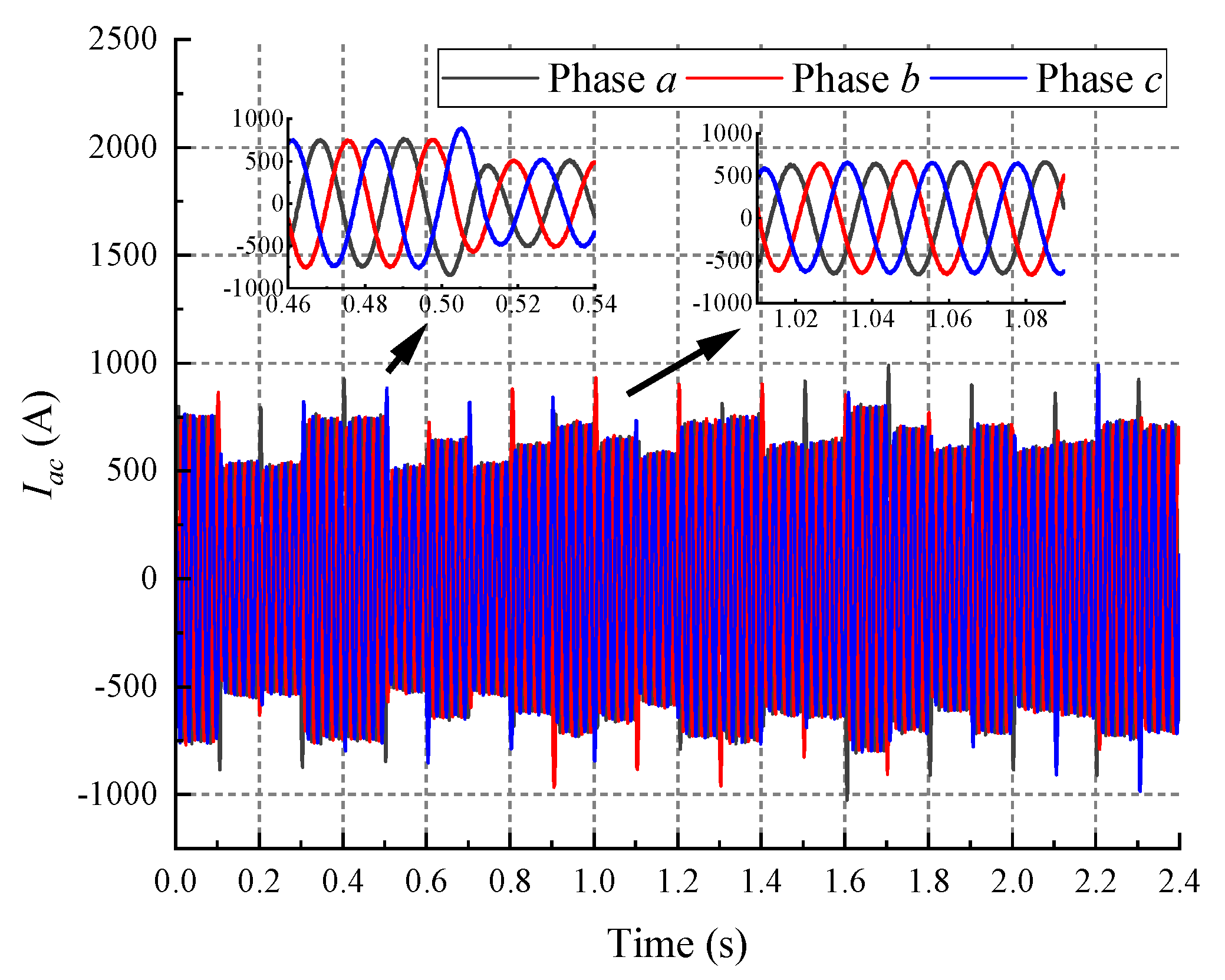
To illustrate the effectiveness of power optimization in controlling the power flow, the proposed method also displays the current flowing between the microgrid bus and the grid, as shown in Figure 14. The results show that the system can accurately track changes in power dispatch and maintain a stable current output while exchanging energy with the grid. This demonstrates the reliability of the proposed method while maintaining a relatively stable voltage.
5. Conclusions
This paper proposes a method to eliminate the impact of randomness in a microgrid system caused by new energy generation and load demand. The method uses scenario generation and probability distribution to create simulation scenarios of system uncertainty. A cost function is established for the generated scenarios, and the PSO algorithm is used for optimization to obtain the optimal cost considering the randomness of power generation and consumption. The study also includes a collaborative hierarchical control strategy for various distributed power sources and loads in each subgrid. The simulation results indicate that the hybrid microgrid can stably run in both islanded and grid-connected modes, ensuring reliable voltage supplies from AC and DC bus even with changes in load power and output of new energy. The upcoming work for this paper is as follows: (1) To create an integrated tertiary and optimization control system for AC-DC hybrid microgrids, taking into account the differences between power guidance values and operating speeds on both sides; (2) While previous research has focused on control superimposition from bottom to top, there is also a need to explore and study the generation of top-down guidance signals; (3) To comprehensively solve the optimization algorithms of complex microgrid systems and uncover more adaptability and possibilities, it is necessary to utilize more intelligent algorithms and their combinations; (4) Optimization design and problem solving often bring about huge and heavy data and scenario set processing issues. Knowledge of how to effectively support the reduction of scenario sets to reduce the workload and whether reduced scenarios can still represent practical cases still needs further improvement.
Author Contributions
Conceptualization, Y.S.; methodology, Y.S. and L.M.; software, L.M.; validation, L.M. and X.Y.; writing—original draft preparation, L.M. and X.Y.; writing—review and editing, Y.S. All authors have read and agreed to the published version of the manuscript.
Funding
This work was supported in part by the Shanghai Sailing Program, China under Grant 21YF1400100, and in part by the Fundamental Research Funds for the Central Universities, China under Grant 2232021D-38.
Data Availability Statement
Not applicable.
Conflicts of Interest
The authors declare no conflict of interest.
References
- Ilyushin, P.; Volnyi, V.; Suslov, K.; Filippov, S. State-of-the-Art Literature Review of Power Flow Control Methods for Low-Voltage AC and AC-DC Microgrids. Energies 2023, 16, 3153. [Google Scholar] [CrossRef]
- Guerrero, J.M.; Vasquez, J.C.; Matas, J.; De Vicuña, L.G.; Castilla, M. Hierarchical Control of Droop-Controlled AC and DC Microgrids—A General Approach toward Standardization. IEEE Trans. Ind. Electron. 2011, 58, 158–172. [Google Scholar] [CrossRef]
- Qin, D.; Chen, Y.; Zhang, Z.; Enslin, J. A Hierarchical Microgrid Protection Scheme Using Hybrid Breakers. In Proceedings of the 2021 IEEE 12th International Symposium on Power Electronics for Distributed Generation Systems, PEDG 2021, Online, 28 June–1 July 2021; Institute of Electrical and Electronics Engineers Inc.: Interlaken, Switzerland, 2021. [Google Scholar]
- Han, Y.; Zhang, K.; Li, H.; Coelho, E.A.A.; Guerrero, J.M. MAS-Based Distributed Coordinated Control and Optimization in Microgrid and Microgrid Clusters: A Comprehensive Overview. IEEE Trans. Power Electron. 2018, 33, 6488–6508. [Google Scholar] [CrossRef] [Green Version]
- Raya-Armenta, J.M.; Bazmohammadi, N.; Avina-Cervantes, J.G.; Sáez, D.; Vasquez, J.C.; Guerrero, J.M. Energy Management System Optimization in Islanded Microgrids: An Overview and Future Trends. Renew. Sustain. Energy Rev. 2021, 149, 111327. [Google Scholar] [CrossRef]
- Zhang, Y.; Gatsis, N.; Giannakis, G.B. Robust Energy Management for Microgrids with High-Penetration Renewables. IEEE Trans. Sustain. Energy 2013, 4, 944–953. [Google Scholar] [CrossRef] [Green Version]
- Nguyen, T.A.; Crow, M.L. Stochastic Optimization of Renewable-Based Microgrid Operation Incorporating Battery Operating Cost. IEEE Trans. Power Syst. 2016, 31, 2289–2296. [Google Scholar] [CrossRef]
- Hu, W.; Wang, P.; Gooi, H.B. Toward Optimal Energy Management of Microgrids via Robust Two-Stage Optimization. IEEE Trans. Smart Grid 2018, 9, 1161–1174. [Google Scholar] [CrossRef]
- Javed, H.; Muqeet, H.A.; Shehzad, M.; Jamil, M.; Khan, A.A.; Guerrero, J.M. Optimal Energy Management of a Campus Microgrid Considering Financial and Economic Analysis with Demand Response Strategies. Energies 2021, 14, 8501. [Google Scholar] [CrossRef]
- Ahmad, J.; Tahir, M.; Mazumder, S.K. Improved Dynamic Performance and Hierarchical Energy Management of Microgrids with Energy Routing. IEEE Trans. Ind. Inf. 2019, 15, 3218–3229. [Google Scholar] [CrossRef]
- Hai, T.; Zhou, J.; Khaki, M. Optimal Planning and Design of Integrated Energy Systems in a Microgrid Incorporating Electric Vehicles and Fuel Cell System. J. Power Sources 2023, 561, 232694. [Google Scholar] [CrossRef]
- Qin, D.; Sun, Q.; Wang, R.; Ma, D.; Liu, M. Adaptive Bidirectional Droop Control for Electric Vehicles Parking with Vehicle-to-Grid Service in Microgrid. CSEE J. Power Energy Syst. 2020, 6, 793–805. [Google Scholar] [CrossRef]
- Tian, P.; Xiao, X.; Wang, K.; Ding, R. A Hierarchical Energy Management System Based on Hierarchical Optimization for Microgrid Community Economic Operation. IEEE Trans. Smart Grid 2016, 7, 2230–2241. [Google Scholar] [CrossRef]
- Yang, X.; Liu, S.; Zhang, L.; Su, J.; Ye, T. Design and Analysis of a Renewable Energy Power System for Shale Oil Exploitation Using Hierarchical Optimization. Energy 2020, 206, 118078. [Google Scholar] [CrossRef]
- Jani, A.; Karimi, H.; Jadid, S. Multi-Time Scale Energy Management of Multi-Microgrid Systems Considering Energy Storage Systems: A Multi-Objective Two-Stage Optimization Framework. J. Energy Storage 2022, 51, 104554. [Google Scholar] [CrossRef]
- Luo, E.; Cong, P.; Lu, H.; Li, Y. Two-Stage Hierarchical Congestion Management Method for Active Distribution Networks with Multi-Type Distributed Energy Resources. IEEE Access 2020, 8, 120309–120320. [Google Scholar] [CrossRef]
- Zhao, J.; Wang, W.; Guo, C. Hierarchical Optimal Configuration of Multi-Energy Microgrids System Considering Energy Management in Electricity Market Environment. Int. J. Electr. Power Energy Syst. 2023, 144, 108572. [Google Scholar] [CrossRef]
- Velasquez, M.A.; Torres-Pérez, O.; Quijano, N.; Cadena, Á. Hierarchical Dispatch of Multiple Microgrids Using Nodal Price: An Approach from Consensus and Replicator Dynamics. J. Mod. Power Syst. Clean Energy 2019, 7, 1573–1584. [Google Scholar] [CrossRef] [Green Version]
- Hossain, M.A.; Pota, H.R.; Squartini, S.; Abdou, A.F. Modified PSO Algorithm for Real-Time Energy Management in Grid-Connected Microgrids. Renew. Energy 2019, 136, 746–757. [Google Scholar] [CrossRef]
- Hu, J.; Shan, Y.; Xu, Y.; Guerrero, J.M. A Coordinated Control of Hybrid Ac/Dc Microgrids with PV-Wind-Battery under Variable Generation and Load Conditions. Int. J. Electr. Power Energy Syst. 2019, 104, 583–592. [Google Scholar] [CrossRef] [Green Version]
- Shakiba, F.M.; Shojaee, M.; Azizi, S.M.; Zhou, M. Real-Time Sensing and Fault Diagnosis for Transmission Lines. Int. J. Netw. Dyn. Intell. 2022, 1, 36–47. [Google Scholar] [CrossRef]
- Kreishan, M.Z.; Zobaa, A.F. Optimal Allocation and Operation of Droop-Controlled Islanded Microgrids: A Review. Energies 2021, 14, 4653. [Google Scholar] [CrossRef]
- Fu, Y.; Zhang, Z.; Mi, Y.; Li, Z.; Li, F. Droop Control for DC Multi-Microgrids Based on Local Adaptive Fuzzy Approach and Global Power Allocation Correction. IEEE Trans. Smart Grid 2018, 10, 5468–5478. [Google Scholar] [CrossRef]
- Meng, L.; Dragicevic, T.; Vasquez, J.C.; Guerrero, J.M. Tertiary and Secondary Control Levels for Efficiency Optimization and System Damping in Droop Controlled DC-DC Converters. IEEE Trans. Smart Grid 2015, 6, 2615–2626. [Google Scholar] [CrossRef] [Green Version]
- Su, Y.; Cai, H.; Huang, J. The Cooperative Output Regulation by the Distributed Observer Approach. Int. J. Netw. Dyn. Intell. 2022, 1, 20–35. [Google Scholar] [CrossRef]
- Wang, W.; Ikegaya, N.; Okaze, T. Comparing Weibull Distribution Method and Gram–Charlier Series Method within the Context of Estimating Low-Occurrence Strong Wind Speed of Idealized Building Cases. J. Wind Eng. Ind. Aerodyn. 2023, 236, 105401. [Google Scholar] [CrossRef]
- Bagheri, F.; Dagdougui, H.; Gendreau, M. Stochastic Optimization and Scenario Generation for Peak Load Shaving in Smart District Microgrid: Sizing and Operation. Energy Build. 2022, 275, 112426. [Google Scholar] [CrossRef]
- He, Y.; Wu, H.; Ding, M.; Bi, R.; Hua, Y. Reduction Method for Multi-Period Time Series Scenarios of Wind Power. Electr. Power Syst. Res. 2023, 214, 108813. [Google Scholar] [CrossRef]
- Morales, J.M.; Pineda, S.; Conejo, A.J.; Carrión, M. Scenario Reduction for Futures Market Trading in Electricity Markets. IEEE Trans. Power Syst. 2009, 24, 878–888. [Google Scholar] [CrossRef]
- Zhang, Z.; Altalbawy, F.M.A.; Al-Bahrani, M.; Riadi, Y. Regret-Based Multi-Objective Optimization of Carbon Capture Facility in CHP-Based Microgrid with Carbon Dioxide Cycling. J. Clean. Prod. 2023, 384, 135632. [Google Scholar] [CrossRef]
- Dou, C.; Zhou, X.; Zhang, T.; Xu, S. Economic Optimization Dispatching Strategy of Microgrid for Promoting Photoelectric Consumption Considering Cogeneration and Demand Response. J. Mod. Power Syst. Clean Energy 2020, 8, 557–563. [Google Scholar] [CrossRef]
- Lai, J.C.T.; Chung, H.S.H.; He, Y.; Wu, W.; Blaabjerg, F. Wideband Series Harmonic Voltage Compensator Using Look-Ahead State Trajectory Prediction for Network Stability Enhancement and Condition Monitoring. IEEE Trans. Power Electron. 2023, 38, 5266–5282. [Google Scholar] [CrossRef]
- Alahakoon, S.; Roy, R.B.; Arachchillage, S.J. Optimizing Load Frequency Control in Standalone Marine Microgrids Using Meta-Heuristic Techniques. Energies 2023, 16, 4846. [Google Scholar] [CrossRef]
- Abbasi, A.; Sultan, K.; Afsar, S.; Aziz, M.A.; Khalid, H.A. Optimal Demand Response Using Battery Storage Systems and Electric Vehicles in Community Home Energy Management System-Based Microgrids. Energies 2023, 16, 5024. [Google Scholar] [CrossRef]
- Khosravi, N.; Echalih, S.; Hekss, Z.; Baghbanzadeh, R.; Messaoudi, M.; Shahideipour, M. A New Approach to Enhance the Operation of M-UPQC Proportional-Integral Multiresonant Controller Based on the Optimization Methods for a Stand-Alone AC Microgrid. IEEE Trans. Power Electron. 2023, 38, 3765–3774. [Google Scholar] [CrossRef]
- Gonzales-Zurita, O.; Andino, O.L.; Clairand, J.M.; Escriva-Escriva, G. PSO Tuning of a Second-Order Sliding Mode Controller for Adjusting Active Standard Power Levels for Smart Inverter Applications. IEEE Trans. Smart Grid 2023, 1. [Google Scholar] [CrossRef]
- Alomoush, M.I. Optimal Combined Heat and Power Economic Dispatch Using Stochastic Fractal Search Algorithm. J. Mod. Power Syst. Clean Energy 2020, 8, 276–286. [Google Scholar] [CrossRef]
- Gheisarnejad, M.; Akhbari, A.; Rahimi, M.; Andresen, B.; Khooban, M.H. Reducing Impact of Constant Power Loads on DC Energy Systems by Artificial Intelligence. IEEE Trans. Circuits Syst. II Express Briefs 2022, 69, 4974–4978. [Google Scholar] [CrossRef]
- Montoya, O.D.; Gil-Gonzalez, W.; Garces, A. Optimal Power Flow on DC Microgrids: A Quadratic Convex Approximation. IEEE Trans. Circuits Syst. II Express Briefs 2019, 66, 1018–1022. [Google Scholar] [CrossRef]
Figure 1.
A hybrid microgrid with AC and DC subgrids.
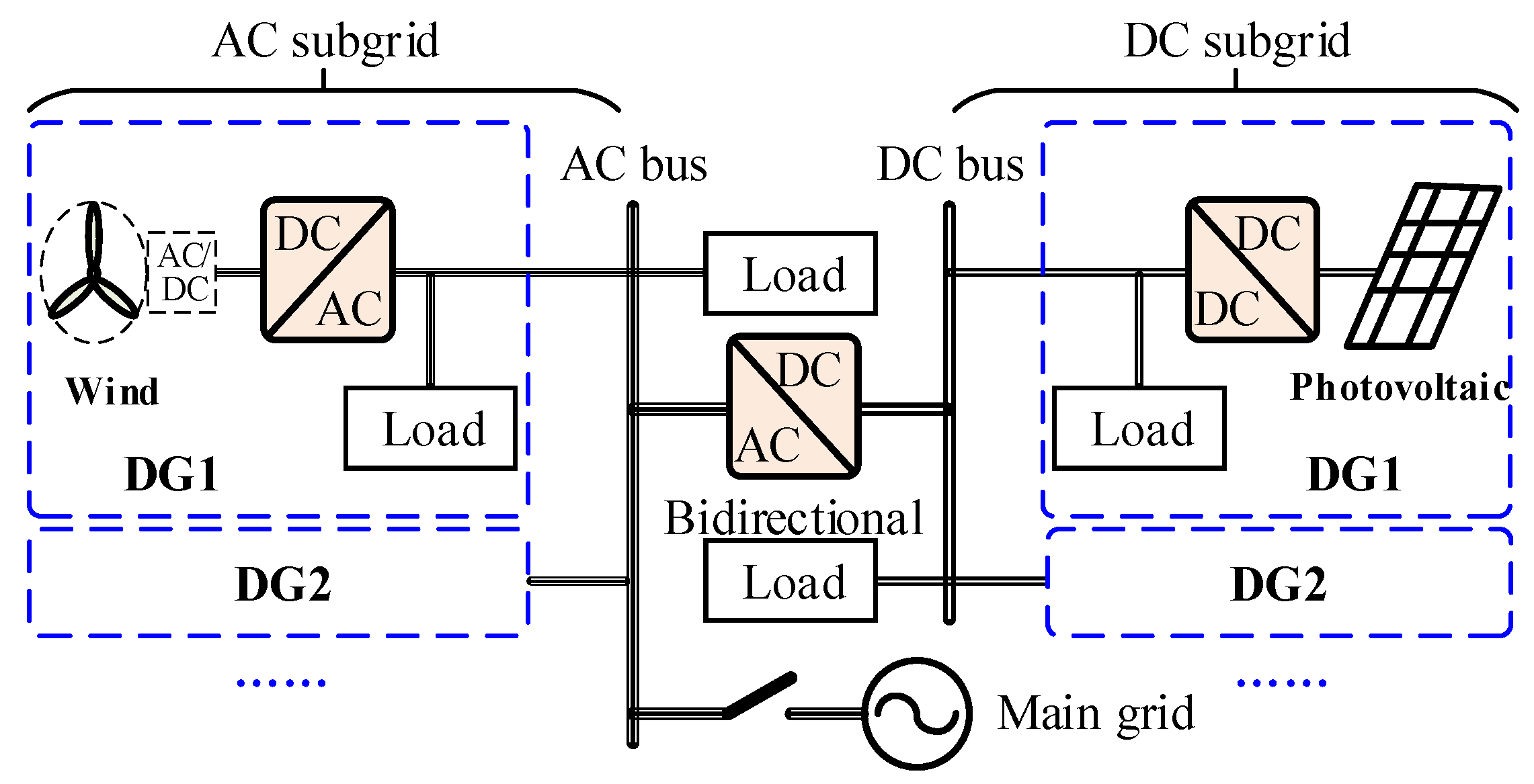
Figure 2.
Overall control block diagram.

Figure 3.
Screenshot of the simulation model for microgrid and hierarchical control.
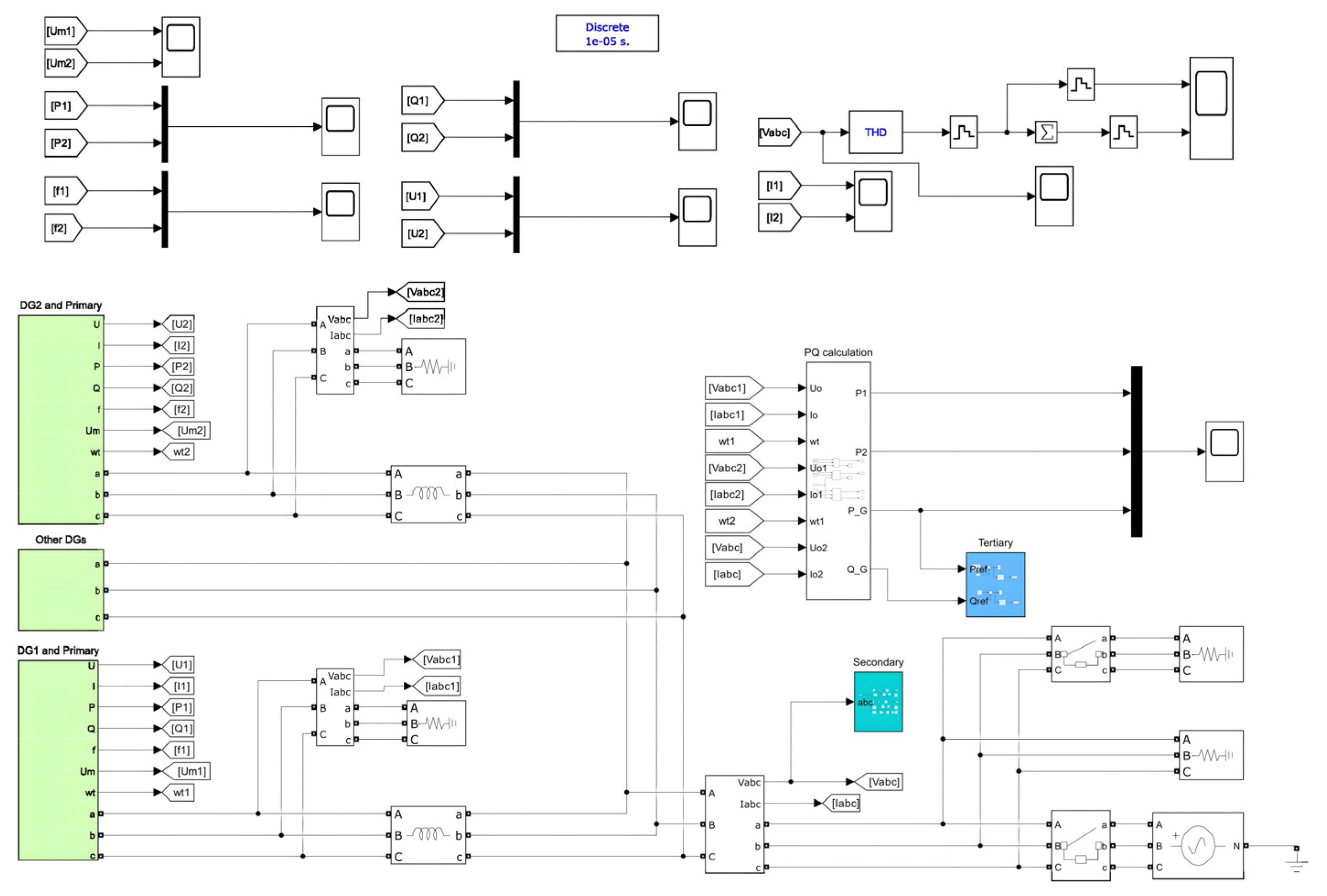
Figure 4.
AC subgrid performance with only primary control and with both primary and secondary controls. (a) Frequency. (b) Voltage.
Figure 4.
AC subgrid performance with only primary control and with both primary and secondary controls. (a) Frequency. (b) Voltage.

Figure 5.
DC subgrid performance with only primary control and with both primary and secondary controls. (a) Under primary control. (b) Under secondary control.
Figure 5.
DC subgrid performance with only primary control and with both primary and secondary controls. (a) Under primary control. (b) Under secondary control.
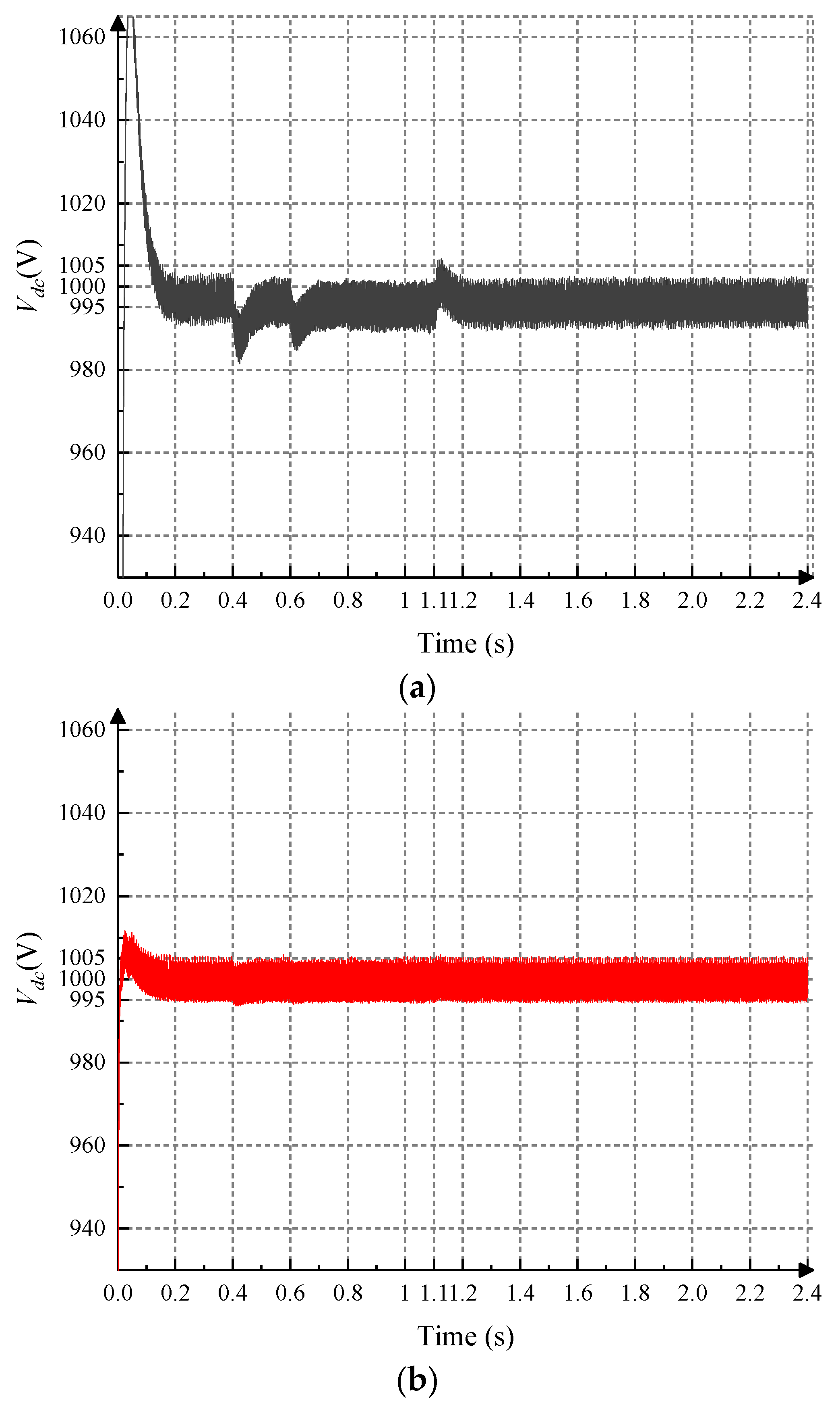
Figure 6.
Power distribution of microgrid with only primary control and with both primary and secondary controls. (a) DC subgrid power. (b) AC subgrid active power. (c) AC subgrid reactive power.
Figure 6.
Power distribution of microgrid with only primary control and with both primary and secondary controls. (a) DC subgrid power. (b) AC subgrid active power. (c) AC subgrid reactive power.

Figure 7.
Scenario generation results considering uncertainty. (a) Wind power. (b) Photovoltaic power. (c) Load demand.
Figure 7.
Scenario generation results considering uncertainty. (a) Wind power. (b) Photovoltaic power. (c) Load demand.
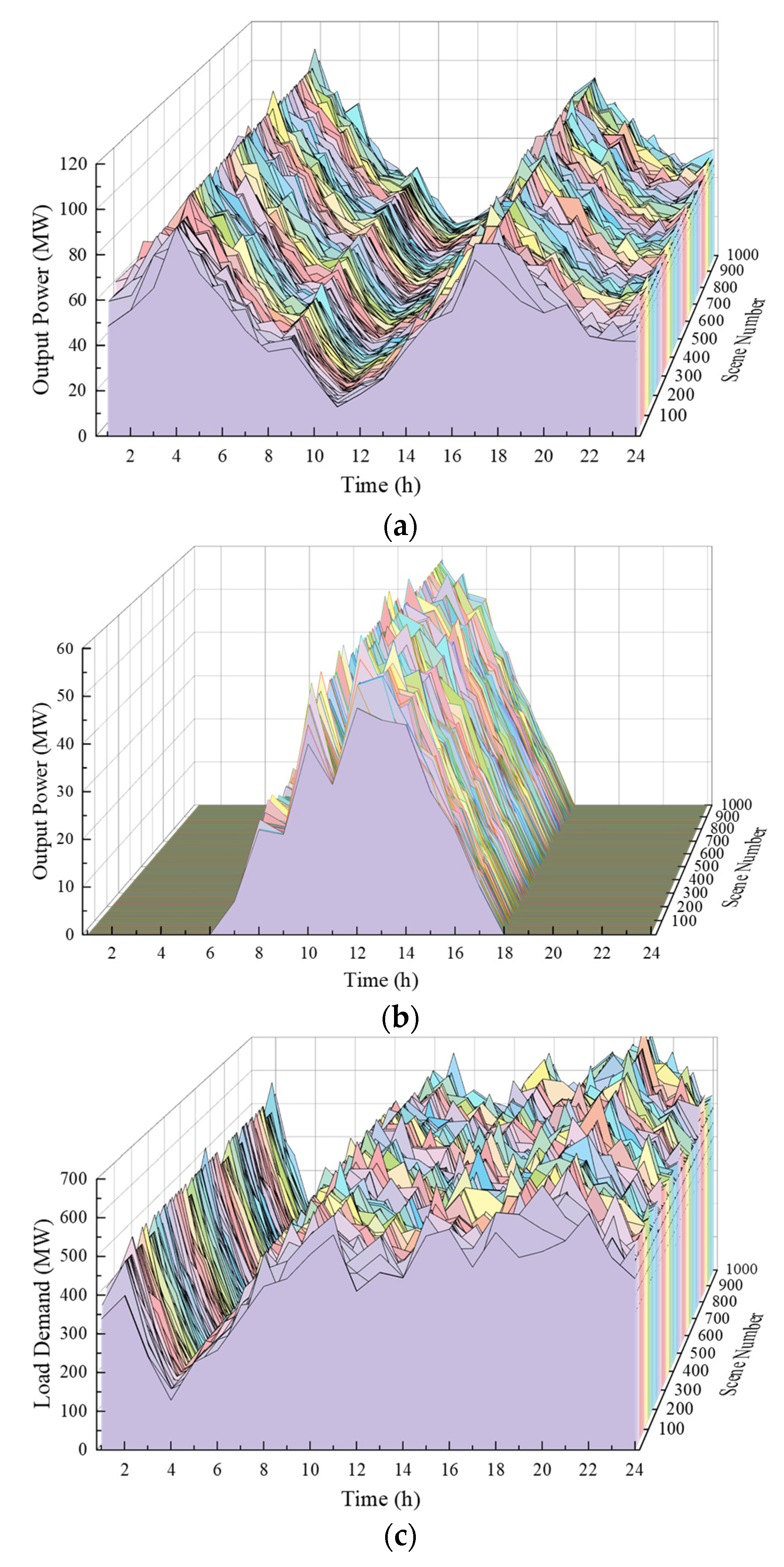
Figure 8.
Scenario reduction results considering uncertainty. (a) Wind power. (b) Photovoltaic power. (c) Load demand.
Figure 8.
Scenario reduction results considering uncertainty. (a) Wind power. (b) Photovoltaic power. (c) Load demand.
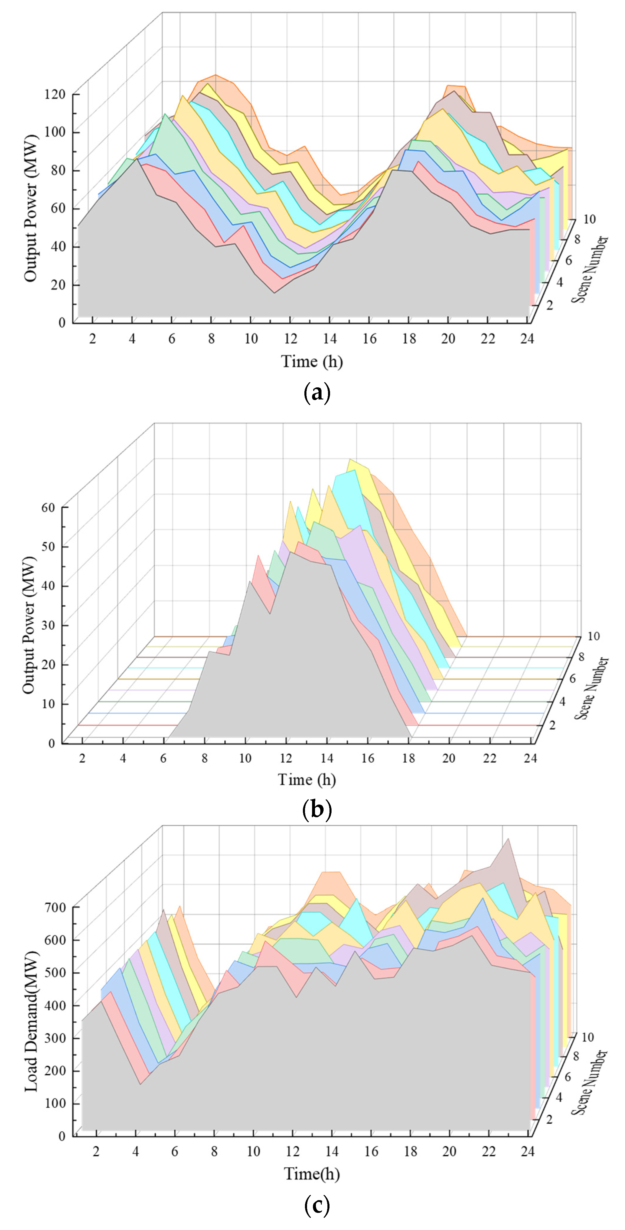
Figure 9.
Operational Area Map of CHP Units in Microgrid. (a) CHP1. (b) CHP2.

Figure 10.
Convergence of PSO algorithm for the optimal solution considering load and wind power uncertainty.
Figure 10.
Convergence of PSO algorithm for the optimal solution considering load and wind power uncertainty.

Figure 11.
Optimized power values with the reduction in electricity generation costs.

Figure 12.
System performance under the action of tertiary control. (a) Frequency. (b) Voltage.

Figure 13.
System performance comparison between proposed tertiary control and low/high constant power control scenario. (a) Frequency. (b) Voltage.
Figure 13.
System performance comparison between proposed tertiary control and low/high constant power control scenario. (a) Frequency. (b) Voltage.

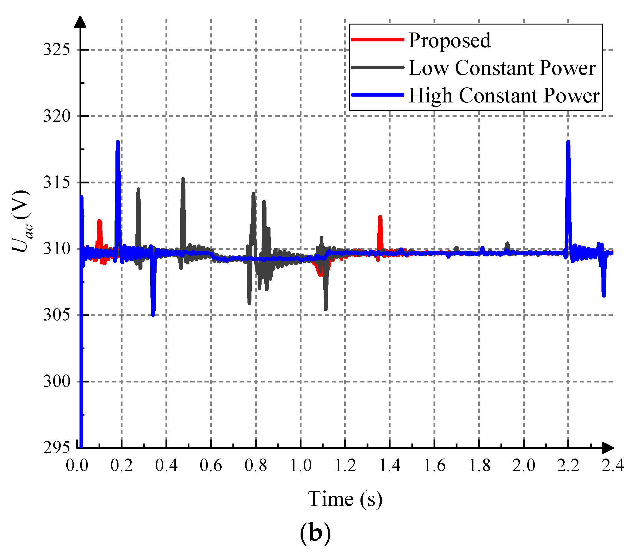
Figure 14.
Current flow between the microgrid bus and main grid.

Table 1.
Microgrid system configuration and control parameters.
| Description | Value |
|---|---|
| Primary Control | |
| DC DG1 and 2 | Rd1, Rd2 = 0.3 |
| AC DG1 | m1 = 3/70,000; n1 = 4/11,000 |
| AC DG2 | m2 = 3/80,000; n2 = 1/3000 |
| System frequency | 50 Hz |
| System voltage | 380 V (p-p, rms) |
| Secondary Control | |
| DC DG1 and 2 | KpV = 10; KiV = 70 |
| AC DG1 and 2 frequency | Kpω = 0.447; Kiω = 47 |
| AC DG1 and 2 bus voltage | KpE = 0.18; KiE = 77 |
| Tertiary Control | |
| AC DG1 and 2 frequency | Kpp = 0.003; KiP = 0.8 |
| AC DG1 and 2 bus voltage | KpQ = 100; KiQ = 3000 |
Table 2.
Microgrid CHP unit cost parameters.
| Unit Number | ||||||
|---|---|---|---|---|---|---|
| CHP1 | 0.0352 | 13.7 | 2650 | 0.028 | 4.3 | 0.029 |
| CHP2 | 0.0423 | 43 | 1250 | 0.032 | 0.7 | 0.009 |
Table 3.
Cost parameters for microgrid pure generating units.
| Unit Number | aip | bip | cip | dip | eip | Pipmin | Pipmax |
|---|---|---|---|---|---|---|---|
| Unit1 | 0.007 | 2.2 | 25 | 100 | 0.045 | 10 | 75 |
| Unit2 | 0.004 | 1.9 | 60 | 140 | 0.038 | 20 | 125 |
| Unit3 | 0.0015 | 2.4 | 100 | 160 | 0.041 | 30 | 175 |
| Unit4 | 0.0012 | 2.1 | 120 | 180 | 0.043 | 40 | 250 |
Table 4.
Cost parameters of microgrid pure heat generation units.
| Unit Number | akh | bkh | ckh | Hkhmax | Hkhmin |
|---|---|---|---|---|---|
| Thermal power unit | 0.036 | 2.0124 | 950 | 2695.2 | 0 |
Table 5.
Optimal total cost under microgrid optimization.
| Optimal Cost Value | Average Cost Value | Maximum Cost Value | |
|---|---|---|---|
| Cost (¥) | 452,044.6317 | 525,045.2684 | 643,369.1997 |
Disclaimer/Publisher’s Note: The statements, opinions and data contained in all publications are solely those of the individual author(s) and contributor(s) and not of MDPI and/or the editor(s). MDPI and/or the editor(s) disclaim responsibility for any injury to people or property resulting from any ideas, methods, instructions or products referred to in the content. |
© 2023 by the authors. Licensee MDPI, Basel, Switzerland. This article is an open access article distributed under the terms and conditions of the Creative Commons Attribution (CC BY) license (https://creativecommons.org/licenses/by/4.0/).
Share and Cite
MDPI and ACS Style
Shan, Y.; Ma, L.; Yu, X. Hierarchical Control and Economic Optimization of Microgrids Considering the Randomness of Power Generation and Load Demand. Energies 2023, 16, 5503. https://doi.org/10.3390/en16145503
AMA Style
Shan Y, Ma L, Yu X. Hierarchical Control and Economic Optimization of Microgrids Considering the Randomness of Power Generation and Load Demand. Energies. 2023; 16(14):5503. https://doi.org/10.3390/en16145503
Chicago/Turabian StyleShan, Yinghao, Liqian Ma, and Xiangkai Yu. 2023. "Hierarchical Control and Economic Optimization of Microgrids Considering the Randomness of Power Generation and Load Demand" Energies 16, no. 14: 5503. https://doi.org/10.3390/en16145503
Note that from the first issue of 2016, this journal uses article numbers instead of page numbers. See further details here.