
PIDD2 Control of Large Wind Turbines’ Pitch Angle
1
School of Control & Computer Engineering, North China Electric Power University, Beijing 102206, China
2
School of Electrical and Control Engineering, North China University of Technology, Beijing 100144, China
*
Author to whom correspondence should be addressed.
Energies 2023, 16(13), 5096; https://doi.org/10.3390/en16135096
Submission received: 7 June 2023
/
Revised: 19 June 2023
/
Accepted: 21 June 2023
/
Published: 1 July 2023
(This article belongs to the Special Issue Advanced Control Technology of Integrated Wind and Wave Energy Conversion System)
Abstract
:The pitch control system has a profound impact on the development of wind energy, and yet a delay or non-minimum phase can weaken its performance. Thus, there is a strong incentive to enhance pitch control technology in order to counteract the negative effects of unidentified delays and non-minimum phase characteristics. To reduce the complexity of the parameter-tuning process and improve the performance of the system, in this paper, we propose a novel control method for wind turbine pitch angle with time delays. Specifically, the proposed control method is state-space PIDD2, which is based on internal model control (IMC) and the open-loop system step response. Then, considering the tracking, disturbance rejection and measurement noise, the proposed controller is verified through simulations. The simulation results demonstrate that the state-space PIDD2 (SS-PIDD2) can provide a trade-off between robustness, time domain performance and measurement noise attenuation and effectively improve pitch control performance in contrast to series PID and PI control methods.
1. Introduction
Renewable energy sources such as wind [1,2] and photovoltaic energy [3,4] have developed rapidly in recent years and have become some of the most feasible ways to meet soaring energy demands and address environmental concerns. Pitch control performs an indispensable function in the control of wind power systems, which is critical for maintaining the stable power output of wind turbines at variable wind speeds. To date, some pitch control methods have been developed, including but not limited to the gain scheduling method [5], adaptive nonlinear sliding mode method [6], fuzzy logic control method [7], linear matrix inequality (LMI) method [8], linear quadratic regulator (LQR) [9] or linear quadratic Gaussian (LQG) control method [10], the PI control [11] and PID control methods [12] and so on. With the increasing power generation capacity of wind turbines and the expansion of the wind turbine blade scale, as well as the influence of factors such as model uncertainty, sometimes the above methods cannot effectively address practical problems; thus, it is essential to devise a valid and reliable control measure to achieve a satisfactory performance [13].
Proportional–integral–derivative (PID) control is a widely used method for controlling industrial processes and engineering applications due to its simplicity and versatility [14]. PID control is a feedback control mechanism that regulates a process that is variable by adjusting a control variable in response to the error between the desired and actual values of the process variable. The proportional term provides a direct response to the error, the integral term accounts for the cumulative error over time, and the derivative term anticipates future changes in the error. The combination of these terms allows PID controllers to be used in pitch control systems. Specifically, the authors of [15] utilized a graphical technique to determine the stability domain of the PI controller and found suitable parameters for the pitch control system, which is a complex procedure aiming to find the stability domain. The authors of [16] determined the selection range of PI controller parameters when the gain and phase margin was satisfied, and yet the unpredictability of the actual operation increased the difficulty of controller design. The authors of [17] designed a pitch controller based on particle swarm optimization (PSO) and radial basis function neural network (RBFNN). Since this method requires data set support and the training process is sluggish, it is not conducive to practical engineering applications. In addition, there are many studies on pitch control systems: for example, the authors of [18] designed delay estimators and compensators and adopted PI and PID controllers for a wind turbine system; the authors of [19] analyzed the and PID controller for the uncertainty problem of wind turbine systems; and the authors of [20] provided a series PID controller designed for the dynamic characteristics of oscillations in wind turbine systems. However, these techniques often require complex mathematical computations, a large amount of information and substantial computational time and computing resources, making the design of these controllers challenging for real-time systems with variable system parameters and interval models. Furthermore, due to the higher-order oscillation characteristics of the wind turbine system, the disturbance rejection of the above method is not good, and the noise attenuation performance is not taken into account.
As is well-known, the internal model control (IMC) technique [21,22] has attracted widespread attention because of its sole tuning parameter () and good stability and control effect. While the control performance of the IMC is recognized, most of the actual industrial processes exhibit oscillation characteristics, as is the case for the wind turbine pitch control system studied in this paper. As a consequence, the IMC-PID is widely used in the field of industrial processes. IMC-PID controllers for oscillatory second-order processes with dead time (SOPDT) are proposed in [23,24]. The authors of [25] modified the integral form of the IMC-PID tuning criterion and obtained a simple tuning formula, and the controller parameters met the requirements of IAE, TV, and robustness. Additionally, the IMC fractional-order PID controller (FOPID) [26,27] has also been investigated by academics. In summary, we can build on this foundation to research wind turbine pitch control systems.
Notwithstanding the fact that the application of PID is universal, it is unable to meet the actual demand in some cases [28]. To improve the performance of conventional PID, a new conventional controller named proportional–integral–double derivative (PIDD2) is widely used [29,30]. Unfortunately, the PIDD2 controller has not discussed been in regard to wind turbine pitch control systems (non-linear, higher-order oscillation with time delay characteristics). For this reason, this paper makes a bold attempt to consider robustness, disturbance rejection and noise attenuation performance in using the above IMC method to tune PIDD2.
The contributions of this paper include:
- The development of a new pitch angle with the time delay control method (SS-PIDD2).
- The proposed controller parameters are obtained through the Maclaurin expansion of the IMC and extension of the applicability of the IMC method.
- The proposed controller parameters are determined taking into consideration robustness and noise factors.
- The proposed controller can provide a trade-off between robustness, time domain performance and measurement noise attenuation.
The remainder of this paper consists of four components: Section 2 describes the large wind turbine system model. Section 3 provides an introduction to the PIDD2 controller’s design and implementation. Section 4 analyzes the simulation results of the SS-PIDD2 controller with those of series PID and PI controllers from a performance point of view. Section 5 concludes the analysis of the control effect and offers perspectives on the proposed method.
2. Large Wind Turbine System Model
The typical pitch angle control system consists of two parts: the pitch angle controller and the pitch angle system model. In this section, we focus on the pitch angle system model. Most theoretical studies of modern pitch angle control systems investigate their linearized structures. A basic linear model block diagram of the generation system of the wind turbine is shown in Figure 1.
The transfer function of the pitch control system is defined as follows [17,31]:
where and are the time constants of the wind turbine generation (WTG) model, of which the values depend on the operating conditions of the wind turbine for generation. is the time delay of the process.
According to the different operating conditions of the WTG, the WTG can be divided into three types, WTG1, WTG2 and WTG3 [15,32], and the corresponding model parameters are shown in Table 1.
WTG1: Rotor diameter = 27 m, tower height = 42 m, rated power = 275 MW, operating conditions: wind speed = 15 m/s, pitch angle = 0°.
WTG2: Rotor diameter = 70 m, tower height = 90 m, rated power = 1.5 MW, operating conditions: wind speed = 15 m/s, pitch angle = 0°.
WTG3: Rotor diameter = 15 m, tower height = 25 m, rated power = 50 MW, operating conditions: wind speed = 15 m/s, pitch angle = 0.75°.
Since Equation (1) is a high-order oscillatory plant, its abundant features and the effect of time delay increase the complexity of process control. It is difficult to directly implement Equation (1). To facilitate our research, this complex plant is approximated using the step response of an open-loop system as an oscillatory second-order model with zero plus dead time (SOZPDT) [20]. Table 2 shows the specific parameters of Equation (2).
3. PIDD2 Controller Design and Implementation
PIDD2, as a variant of PID, has a new degree of freedom (differential action) in comparison to PID, which can accelerate the transient and closed-loop performance of the control system and contributes to promoting the phase margin, steady-state accuracy and stability of the controlled plant. As such, in this section, we describe the design and implementation process of the PIDD2 controller in detail.
3.1. Description of the SS-PIDD2 Controller
The PID controller has widespread applicability in industrial process control because of its simple operation, high efficiency and easy implementation. Aiming to overcome the drawbacks of conventional PID controllers and improve their performance, the PIDD2 controller has also gradually become recognized in the industry. PIDD2 has the same structure as PID, except for an additional second-order derivative gain. An ideal PIDD2 controller has the following transfer function form:
where ,, and are the proportional, integral, derivative and double-derivative gain, respectively. PIDD2 control can be written as a state-feedback control law, as follows:
where is the controlled variable, is the manipulated variable, and is the reference input signal:
and the state vector is
and state-feedback gain is
The state vector (6) contains the derivate of . The state variable cannot be measured directly; hence, here, we estimate it in the form of an observer. Thus, we consider a triple-integral model:
Let
Then, Equation (8) can be written in the form of state space:
where
Thus, Equation (12) can be used to estimate .
where is the observer gain:
If is chosen such that is asymptotically stable, then and and . Furthermore, can be calculated using another state , where
Combining Equations (12) and (14), we can obtain the expression for the state estimator as:
where
is the observer gain vector.
When is chosen properly, is asymptotically stable, and
Hence, an ideal PIDD2 controller can be approximated with the following third-order state-space PID (SS-PIDD2) controller.
Thus, the expression for the feedback controller from to becomes:
and is the controller gain vector, as in Equation (7).
Figure 2 shows a basic structural block diagram of the SS-PIDD2. is the weight factor of the setpoint used to reduce the overshoot of the trace response. In general, , and the value of can be regulated according to the actual situation.
3.2. Derivation of SS-PIDD2 Controller Parameters
3.2.1. Internal Model Control (IMC)
Figure 3 shows the structure of the two-degree-of-freedom IMC (TDF-IMC). is the model plant of , is the internal model controller, and is the feedback controller.
The design process of the TDF-IMC controller is as follows [33]:
- (1)
- Factor the plant model into two parts:where is the portion of the minimum phase and is the portion of the model that is not inverted.
- (2)
- The setpoint-tracking controller is defined as follows:where denotes a low-pass filter:where represents the parameter of and represents the relative degree of .
- (3)
- The feedback controller is defined as follows:
The denominator of is a polynomial consisting of the poles of , the disturbance rejection filter has the order , and is the parameter that determines the disturbance-rejecting performance of the controller. The poles of can be canceled with the zeros of , i.e., should satisfy:
Thus, we can obtain the transfer function for the IMC controller as:
3.2.2. The IMC Controller’s Design for the SOZPDT System
The controllers and for Equation (2) are:
Here, is chosen as 3, and , meet Equation (25).
Through the above-mentioned derivation, the final term of Equation (26) is:
From the above derivation, we can cancel the roots of . To obtain a finite-dimensional controller, we take the first-order Padé approximation technique [33,34] to approximate the pure delay.
Then, Equation (29) becomes:
It is worth noting that the selection of and has a significant impact on the control effect of IMC. However, there is no general tuning rule for the selection of and . The authors of [35] mentioned that a small can improve the disturbance rejection performance and tracking performance of the controller and worsen the robustness of the system. Thus, the choice of requires the consideration of robustness issues. For various types of systems, the authors of [36] set the value of based on experience. For the second-order plus time delay (SOPTD) system, the expression of for and , which is only applicable to non-oscillating systems, is given in [37]. The authors of [23] provided a definition of for the underdamped oscillation system. The authors of [33] assumed that the bandwidth is equal to the inverse of and and that the values of and determine the tracking performance and disturbance rejection performance of the closed-loop system. Therefore, in this paper, and are selected under conditions that meet the consideration of robustness and disturbance rejection.
3.2.3. The Derivation of SS-PIDD2 Controller Parameters
To obtain SS-PIDD2 parameters from the IMC, we expand the transfer function as the Maclaurin series with s = 0 and retain the first three terms. The parameters of the SS-PIDD2 can be computed from Equation (31) as:
where
The above Maclaurin expansion can only obtain four parameters of the SS-PIDD2. The method used to set the observer bandwidth is also highlighted in this subsection. As is well known, the observer has the characteristic that it does not depend on the model, so that the observer’s bandwidth can be chosen as not restricted to the model. The authors of [38] referred to the fact that the smaller the value of is, the less sensitive the observer is to noise. The authors of [39] illustrated the relationship between and robustness. For this purpose, we need to take into consideration robustness and noise factors when choosing an appropriate .
4. System Simulation and Analysis
To demonstrate the superiority of the method presented in this paper, simulations were conducted on three distinct pitch control systems for wind turbines, which included the SS-PIDD2, series PID [20], [15] and [6]. All the simulation results are based on MATLAB2021a and the Simulink experimental platform.
The following indices are presented to evaluate the performance and robustness of the controllers:
Robustness index:
where is the open-loop transfer function of the system, and are the maximum sensitivity, and are the sensitivity functions, and denotes the robustness of the system.
Performance index: The performance of the controller was assessed using two measures. The definition of the integral of time and absolute error (ITAE) is:
To assess the control effect of the controller, the total variation (TV) in the controller output is also taken as a performance index.
The TV is used to measure the smoothness of the control signal, and its value should be as small as possible.
As the series PID adds a pre-filter, the same filter was added to the other three controllers for fairness. Figure 4 shows the step response of the WTG1 system, adding a unit step signal with an amplitude of 1 at t = 0 s. From Figure 4, we can see that the response of the SS-PIDD2 can reach a steady state relatively quickly and without overshooting. Figure 5 shows the step response of the WTG1 system, adding a unit step signal with an amplitude of 1 at t = 0 s and an input disturbance signal inserted at t = 25 s. As we can observe, the controller proposed in this paper can achieve a good control effect, and the disturbance rejection is fast and without overshoot. Figure 4 and Figure 5 show the controller in terms of tracking and disturbance rejection, respectively. The dynamic response of the WTG1 system with measurement noise (the amplitude is 0.0001) is shown in Figure 6. In the case of measurement noise, Figure 6 illustrates that the proposed method has minimal volatility compared with the other control methods for both the control output and the system output. The robustness strategy change process is illustrated in Figure 7. The robustness indices of the controllers are 2.9583, 4.4391, 2.8270 and 6.0392, respectively. Hence, the SS-PIDD2 has relatively low robustness and thus has the ability to deal with external uncertainties. Table 3 demonstrates the parameters and performance metrics of the different control methods. From the comprehensive analysis (, ITSE, TV), we can conclude that the SS-PIDD2 controller has a good control performance and can achieve an acceptable control effect.
Remark 1.
Simulation process in Figure 4: A unit step reference signal (the step module in Simulink) with an amplitude of 1 is added to the input (before the pre-filter) of the whole system. The step response on the left side of Figure 4 can be obtained by connecting an oscilloscope to the controller output. The step response on the right side of Figure 4 can be obtained by connecting an oscilloscope to the system output.
Simulation process in Figure 4: The process is the same as in Figure 4, except that a disturbance signal of is added to the controller output and the input of the controlled plant.
Simulation process in Figure 4: Based on Figure 4, a white noise module with an amplitude of 0.0001 is connected at the output end of the system.
Figure 4 is derived from Equation (34), and the values of ITAE and TV are calculated through Equations (35) and (36), respectively.
and are selected under conditions that meet the consideration of robustness and disturbance rejection. The value of takes into account the robustness and the noise factor.
Since the time delay will increase the complexity of the system, to verify the stability of the system, we conducted a simulation study on the uncertainty of the time delay . Here, we consider changing the time delay in Equation (1) by 10%. For WTG1, the simulation results are shown in Figure 8 and Figure 9. When is reduced by 10%, the robustness indices are 2.8134, 6.8300, 3.2044 and 3.5105, respectively; the ITAE indices are 428.1043, 552.4503, 3.4803 × 10³ and 4.2302 × 10³, respectively; and the total variation values are 50, 50, 50.1292 and 91.1828, respectively. When is increased by 10%, the robustness indices are 3.1356, 3.1654, 2.0311 and 3.5699, respectively; the ITAE indices are 428.1043, 552.4504, 3.4810 × 10³ and 939.4192, respectively; and the total variation values are 50, 50, 50.1308 and 50.0295, respectively. Thus, we can draw the same conclusion as above.
For the WTG2 system, Figure 10 (the left) shows the controller output responses. The SS-PIDD2 controller output tends to be stable at 6 s, without overshoot. The series PID controller output response presents a large overshoot, and the stabilization time is the longest. The system output (on the right) leads us to similar conclusions (to those discussed in the previous WTG1), which are not described here. Although it is difficult to see which controller has the best disturbance rejection performance in Figure 11 (adding a unit step signal with an amplitude of 1 at t = 0 s and an input disturbance signal inserted at t = 20 s). In addition, considering the situation with measurement noise (the amplitude is 0.0001), Figure 12 shows that both the controller output and the system output of the SS-PIDD2 controller are least influenced by noise. Figure 13 and Table 4 show that the disturbance rejection performance (ITSE) and robustness () of the SS-PIDD2 controller are the best. The TV indices in Table 4 further demonstrate this. Therefore, we can conclude that the proposed method offers better results for wind turbine pitch angle systems than the other methods.
Remark 2.
Simulation process in Figure 10: A unit step reference signal (the step module in Simulink) with an amplitude of 1 is added to the input (before the pre-filter) of the whole system. The step response on the left side of Figure 10 can be obtained by connecting an oscilloscope to the controller output. The step response on the right side of Figure 10 can be obtained by connecting an oscilloscope to the system output.
Simulation process in Figure 11: The process is the same as in Figure 10, except that a disturbance signal of is added to the controller output and the input of the controlled plant.
Simulation process in Figure 12: Based on Figure 11, a white noise module with an amplitude of 0.0001 is connected at the output end of the system.
For WTG2, the stability simulation results are shown in Figure 14 and Figure 15. When is reduced by 10%, the robustness indices are 2.0288, 2.3827, 3.1003 and 4.0432, respectively; the ITAE indices are 373.5015, 490.5610, 482.8402 and 319.2728, respectively; and the total variation values are 20.0666, 20.0585, 20.0990 and 20.1565, respectively. When is increased by 10%, the robustness indices are 2.0694, 4.4646, 2.5629 and 3.9859, respectively; the ITAE indices are 373.5436, 490.7258, 482.8974 and 319.3154, respectively; and the total variation values are 20.0667, 20.2003, 20.0991 and 20.1567, respectively. Thus, we can also draw the same conclusion as above.
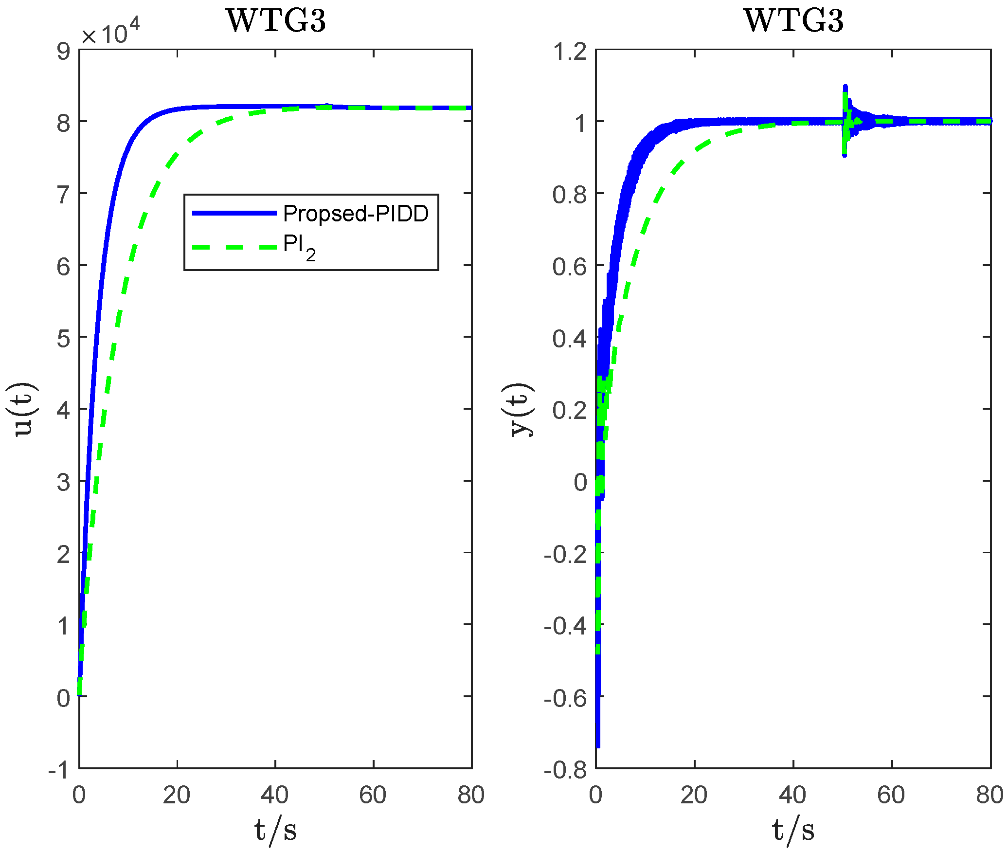
Figure 16 shows the bode plots of the systems. As shown in Figure 16, WTG3 has two oscillation modes, it is more sophisticated than the former two, and higher demands are also placed on the controllers. As the current research on WTG3 is limited to PI control methods, we used both SS-PIDD2 and PI controllers for the simulation comparison analysis. Using a similar process to that mentioned above for WTG1 and WTG2, simulations were performed for the step responses, disturbance response, measurement noise response and robustness change process, respectively. In Figure 17, Figure 18, Figure 19 and Figure 20, we can see that the control speed of the SS-PIDD2 controller is fast and has no overshoot. However, under the conditions of disturbance and measurement noise, there is no obvious advantage in comparison to the SS-PIDD2 controller and PI controller. Moreover, we can see from the performance metrics data in Table 5 that the overall performance (, ITAE and TV) of the SS-PIDD2 controller is satisfactory. In particular, the value of the ITAE clearly shows the disturbance rejection performance of the SS-PIDD2 controller. We can thus state that SS-PIDD2 controllers can also control wind turbine pitch angle systems with non-minimum phases very effectively.
Remark 3.
Simulation process in Figure 17: A unit step reference signal (the step module in Simulink) with an amplitude of 1 is added to the input of the whole system. The step response on the left side of Figure 17 can be obtained by connecting an oscilloscope to the controller output. The step response on the right side of Figure 17 can be obtained by connecting an oscilloscope to the system output.
Simulation process in Figure 18: The process is the same as in Figure 17, except that a disturbance signal is added to the controller output and the input of the controlled plant.
Simulation process in Figure 19: Based on Figure 18, a white noise module with an amplitude of 0.0001 is connected at the output end of the system.
For WTG3, the stability simulation results are shown in Figure 21 and Figure 22. When is reduced by 10%, the robustness indices are 6.3170 and 10.4073, respectively; the ITAE indices are 0.6194 and 2.0623, respectively; and the total variation values are 22.0852 and 22.2214, respectively. When is increased by 10%, the ITAE indices and 3.5253 and 2.0531, respectively; and the total variation values are 32.3195 and 21.5306, respectively. Although the control effect of PIDD2 is less than that of PI at this point, it is generally good.
5. Conclusions
The purpose of the current study was to investigate the application of the SS-PIDD2 controller in wind turbine pitch control systems (non-linear, higher-order oscillation with time delay characteristics). The pitch control system can be approximated using the step response as an oscillatory second-order model with zero plus dead time. While maintaining the characteristic independence of a conventional PID from the plant, we investigated the ideal PIDD2 in the form of a state space. Furthermore, the SS-PIDD2 controller parameters were obtained through Maclaurin expansion of the IMC and self-tuning. The effectiveness of the proposed method was verified through the simulation analysis of three pitch angle models. The results of this study indicate that the SS-PIDD2 controller has a certain research value for research on complex systems, such as pitch control systems (minimum phase and non-minimum phase), which expands the application field of the high-order PID. In practical industrial production, engineers can consider using SS-PIDD2 instead of PI or PID, which are both easy to operate and can achieve the desired control effect.
The present study confirmed previous findings offering a new understanding of PID controllers. A further study should consider SS-PIDD2 control for other aspects of wind turbine systems.
Author Contributions
Conceptualization, X.H.; methodology, X.H.; software, X.H.; validation, X.H.; formal analysis, X.H.; investigation, X.H.; writing—original draft preparation, X.H.; writing—review and editing, X.H. and W.T.; supervision, W.T. and G.H.; project administration, G.H. All authors have read and agreed to the published version of the manuscript.
Funding
This research received no external funding.
Data Availability Statement
Data are obtained in the article.
Conflicts of Interest
The authors declare no conflict of interest.
References
- Carvalho, D.; Rocha, A.; Gómez-Gesteira, M.; Silva Santos, C. Potential impacts of climate change on European wind energy resource under the CMIP5 future climate projections. Renew. Energy 2017, 101, 29–40. [Google Scholar] [CrossRef]
- Wang, H.; Li, G.; Wang, G.; Peng, J.; Jiang, H.; Liu, Y. Deep learning based ensemble approach for probabilistic wind power forecasting. Appl. Energy 2017, 188, 56–70. [Google Scholar] [CrossRef]
- Abdel-Rahim, O.; Funato, H. A novel model predictive control for high gain switched inductor power conditioning system for photovoltaic applications. In Proceedings of the 2014 IEEE Innovative Smart Grid Technologies-Asia (ISGT ASIA), Kuala Lumpur, Malaysia, 20–23 May 2014; IEEE: Kuala Lumpur, Malaysia, 2014; pp. 170–174. [Google Scholar]
- Ahmed, H.Y.; Abdel-Rahim, O.; Ali, Z.M. New High-Gain Transformerless DC/DC Boost Converter System. Electronics 2022, 11, 734. [Google Scholar] [CrossRef]
- Bianchi, F.D.; De Battista, H.; Mantz, R.J. Wind Turbine Control Systems: Principles, Modelling and Gain Scheduling Design; Springer: Berlin/Heidelberg, Germany, 2007; Volume 19. [Google Scholar]
- Yin, X.; Lin, Y.; Li, W.; Gu, Y. Integrated pitch control for wind turbine based on a novel pitch control system. J. Renew. Sustain. Energy 2014, 6, 043106. [Google Scholar] [CrossRef]
- Scherillo, F.; Izzo, L.; Coiro, D.P.; Lauria, D. Fuzzy logic control for a small pitch controlled wind turbine. In Proceedings of the International Symposium on Power Electronics Power Electronics, Electrical Drives, Automation and Motion, 20–22 June 2012; IEEE: Sorrento, Italy, 2012; pp. 588–593. [Google Scholar]
- Hassan, H.; ElShafei, A.; Farag, W.; Saad, M. A robust LMI-based pitch controller for large wind turbines. Renew. Energy 2012, 44, 63–71. [Google Scholar] [CrossRef]
- Park, S.; Nam, Y. Two LQRI based Blade Pitch Controls for Wind Turbines. Energies 2012, 5, 1998–2016. [Google Scholar] [CrossRef]
- Taher, S.A.; Farshadnia, M.; Mozdianfard, M.R. Optimal gain scheduling controller design of a pitch-controlled VS-WECS using DE optimization algorithm. Appl. Soft Comput. 2013, 13, 2215–2223. [Google Scholar] [CrossRef]
- Kim, Y.-S.; Chung, I.-Y.; Moon, S.-I. Tuning of the PI Controller Parameters of a PMSG Wind Turbine to Improve Control Performance under Various Wind Speeds. Energies 2015, 8, 1406–1425. [Google Scholar] [CrossRef] [Green Version]
- Makvana, V.T.; Ahir, R.K.; Patel, D.K.; Jadhav, J.A. Study of PID controller based pitch actuator system for variable speed HAWT using matlab. Int. J. Innov. Res. Sci. Eng. Technol. 2013, 2, 1496–1504. [Google Scholar]
- Cross, P.; Ma, X. Nonlinear system identification for model-based condition monitoring of wind turbines. Renew. Energy 2014, 71, 166–175. [Google Scholar] [CrossRef] [Green Version]
- Kim, M.; Lee, S.-U. PID with a Switching Action Controller for Nonlinear Systems of Second-order Controller Canonical Form. Int. J. Control Autom. Syst. 2021, 19, 2343–2356. [Google Scholar] [CrossRef]
- Wang, J.; Tse, N.; Gao, Z. Synthesis on PI-based pitch controller of large wind turbines generator. Energy Convers. Manag. 2011, 52, 1288–1294. [Google Scholar] [CrossRef]
- Turksoy, O.; Ayasun, S.; Hames, Y.; Sonmez, S. Computation of Robust PI-Based Pitch Controller Parameters for Large Wind Turbines. Can. J. Electr. Comput. Eng. 2020, 43, 57–63. [Google Scholar] [CrossRef]
- Perng, J.-W.; Chen, G.-Y.; Hsieh, S.-C. Optimal PID Controller Design Based on PSO-RBFNN for Wind Turbine Systems. Energies 2014, 7, 191–209. [Google Scholar] [CrossRef] [Green Version]
- Gao, R.; Gao, Z. Pitch control for wind turbine systems using optimization, estimation and compensation. Renew. Energy 2016, 91, 501–515. [Google Scholar] [CrossRef]
- Moradi, H.; Vossoughi, G. Robust control of the variable speed wind turbines in the presence of uncertainties: A comparison between H∞ and PID controllers. Energy 2015, 90, 1508–1521. [Google Scholar] [CrossRef]
- Micic, A.; Matausek, M. Series pid pitch controller of large wind turbines generator. Serbian J. Electr. Eng. 2015, 12, 183–196. [Google Scholar] [CrossRef] [Green Version]
- Saxena, S.; Hote, Y. Advances in internal model control technique: A review and future prospects. IETE Tech. Rev. 2012, 29, 461. [Google Scholar] [CrossRef]
- Saxena, S.; Hote, Y.V. Load Frequency Control in Power Systems via Internal Model Control Scheme and Model-Order Reduction. IEEE Trans. Power Syst. 2013, 28, 2749–2757. [Google Scholar] [CrossRef]
- Chien, I.-L. IMC-PID controller design-an extension. IFAC Proc. Vol. 1988, 21, 147–152. [Google Scholar] [CrossRef]
- Lee, Y.; Park, S.; Lee, M.; Brosilow, C. PID controller tuning for desired closed-loop responses for SI/SO systems. Aiche J. 1998, 44, 106–115. [Google Scholar] [CrossRef]
- Skogestad, S. Simple analytic rules for model reduction and PID controller tuning. J. Process Control 2003, 13, 291–309. [Google Scholar] [CrossRef] [Green Version]
- El-Khazali, R. Fractional-order PIλDμ controller design. Comput. Math. Appl. 2013, 66, 639–646. [Google Scholar] [CrossRef]
- Luo, Y.; Chen, Y.Q.; Wang, C.Y.; Pi, Y.G. Tuning fractional order proportional integral controllers for fractional order systems. J. Process Control 2010, 20, 823–831. [Google Scholar] [CrossRef]
- Jadhav, A.M.; Vadirajacharya, K. Performance Verification of PID Controller in an Interconnected Power System Using Particle Swarm Optimization. Energy Procedia 2012, 14, 2075–2080. [Google Scholar] [CrossRef] [Green Version]
- Simanenkov, A.L.; Rozhkov, S.A.; Borisova, V.A. An algorithm of optimal settings for PIDD 2 D 3 -controllers in ship power plant. In Proceedings of the 2017 IEEE 37th International Conference on Electronics and Nanotechnology (ELNANO), Kyiv, Ukraine, 18–20 April 2017; IEEE: Kyiv, Ukraine, 2017; pp. 152–155. [Google Scholar]
- Khakpour, S.; Mirabbasi, D. Performance evaluation of PIDD controller for automatic generation control in interconnected thermal system with reheat turbine in deregulated environment. In Proceedings of the 2015 2nd International Conference on Knowledge-Based Engineering and Innovation (KBEI), Tehran, Iran, 5–6 November 2015; IEEE: Tehran, Iran, 2015; pp. 1207–1212. [Google Scholar]
- Horn, I.G.; Arulandu, J.R.; Gombas, C.J.; VanAntwerp, J.G.; Braatz, R.D. Improved Filter Design in Internal Model Control. Ind. Eng. Chem. Res. 1996, 35, 3437–3441. [Google Scholar] [CrossRef]
- Suryanarayanan, S.; Dixit, A. On the dynamics of the pitch control loop in horizontal-axis large wind turbines. In Proceedings of the 2005, American Control Conference, 8–10 June 2005; IEEE: Portland, OR, USA, 2005; pp. 686–690. [Google Scholar]
- Tan, W.; Fu, C. Linear Active Disturbance Rejection Control: Analysis and Tuning via IMC. IEEE Trans. Ind. Electron. 2015, 63, 2350–2359. [Google Scholar] [CrossRef]
- Shamsuzzoha, M.; Lee, M. Analytical design of enhanced PID filter controller for integrating and first order unstable processes with time delay. Chem. Eng. Sci. 2008, 63, 2717–2731. [Google Scholar] [CrossRef]
- Chen, D.; Seborg, D.E. PI/PID Controller Design Based on Direct Synthesis and Disturbance Rejection. Ind. Eng. Chem. Res. 2002, 41, 4807–4822. [Google Scholar] [CrossRef]
- Shamsuzzoha, M.; Lee, M. IMC−PID Controller Design for Improved Disturbance Rejection of Time-Delayed Processes. Ind. Eng. Chem. Res. 2007, 46, 2077–2091. [Google Scholar] [CrossRef]
- Wang, Q.; Lu, C.; Pan, W. IMC PID controller tuning for stable and unstable processes with time delay. Chem. Eng. Res. Des. 2016, 105, 120–129. [Google Scholar] [CrossRef]
- Gao, Z. Scaling and bandwidth-parameterization based controller tuning. In Proceedings of the 2003 American Control Conference, Denver, CO, USA, 4–6 June 2003; IEEE: Denver, CO, USA, 2003; Volume 6, pp. 4989–4996. [Google Scholar]
- Zhang, B.; Tan, W.; Li, J. Tuning of linear active disturbance rejection controller with robustness specification. ISA Trans. 2019, 85, 237–246. [Google Scholar] [CrossRef]
Figure 1.
The basic block diagram of the generation system of the wind turbine.

Figure 2.
The block diagram of state−space PIDD2.
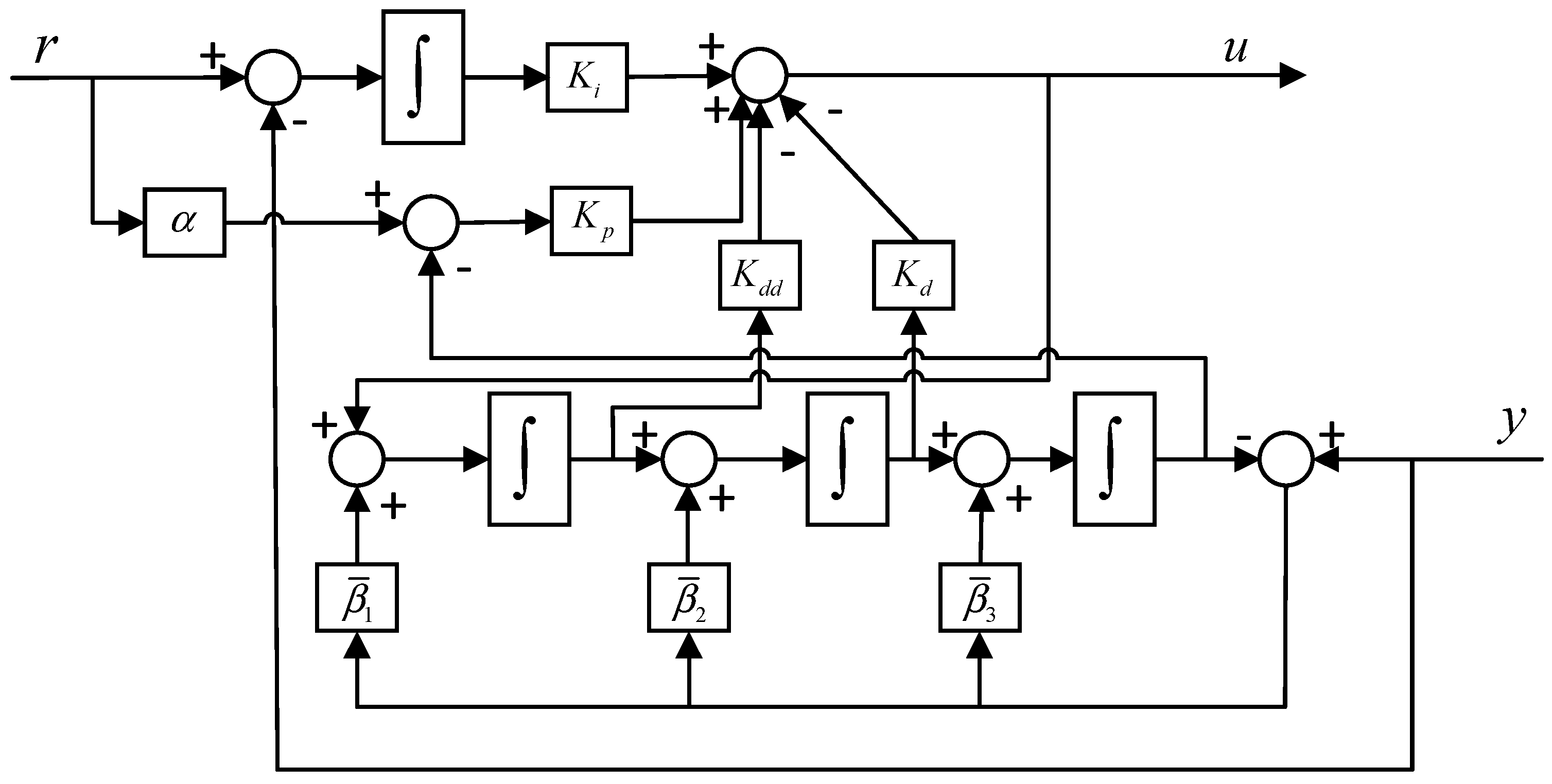
Figure 3.
The block diagram of TDF−IMC.
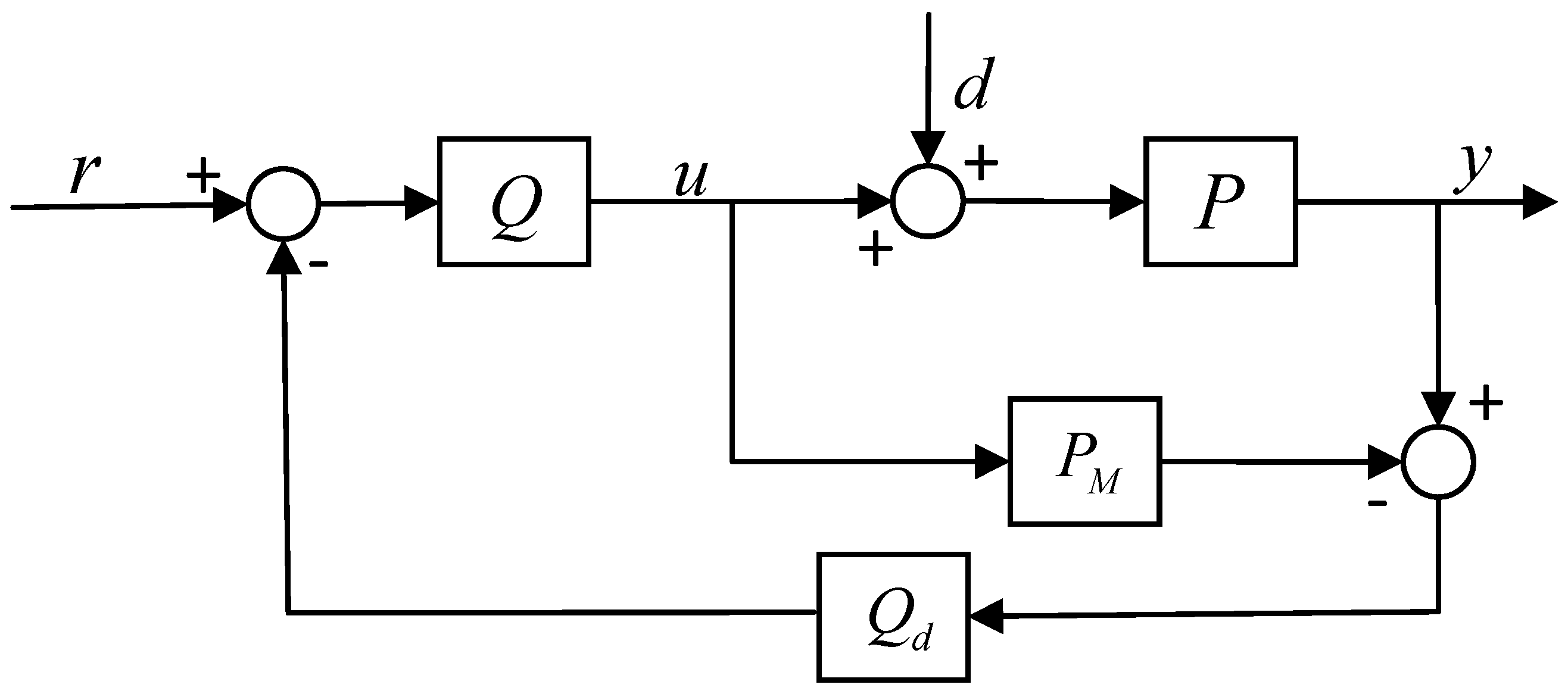
Figure 4.
The dynamic response of the WTG1 system: the controller output dynamic step responses (on the left); the system output dynamic step responses (on the right).
Figure 4.
The dynamic response of the WTG1 system: the controller output dynamic step responses (on the left); the system output dynamic step responses (on the right).
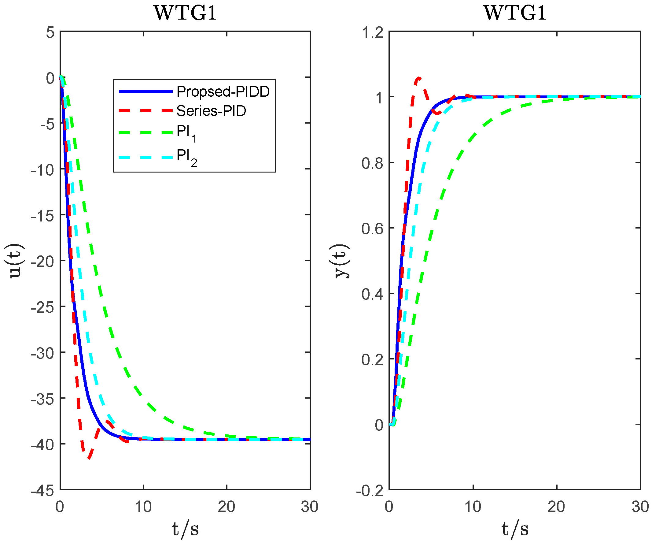
Figure 5.
The dynamic response of the WTG1 system under step disturbance: the controller output dynamic step disturbance responses (on the left); the system output dynamic step disturbance responses (on the right).
Figure 5.
The dynamic response of the WTG1 system under step disturbance: the controller output dynamic step disturbance responses (on the left); the system output dynamic step disturbance responses (on the right).

Figure 6.
The dynamic response of the WTG1 system with noise: the controller output noise responses (on the left); the system output noise responses (on the right).
Figure 6.
The dynamic response of the WTG1 system with noise: the controller output noise responses (on the left); the system output noise responses (on the right).
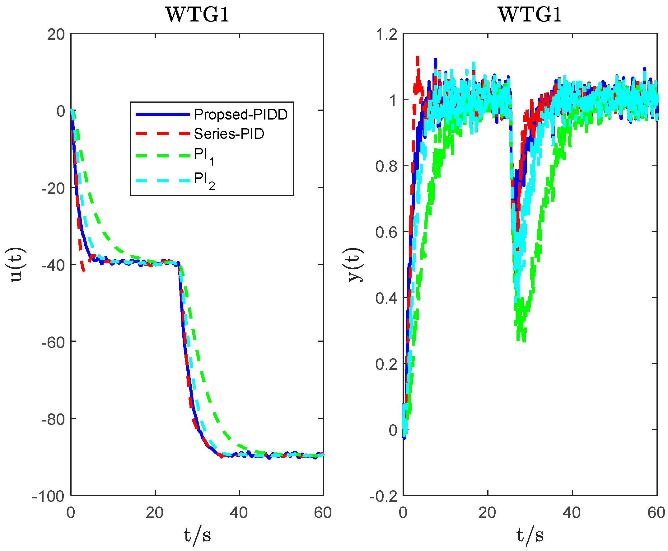
Figure 7.
The robustness change process of the different methods for WTG1.

Figure 8.
The dynamic response of the WTG1 system under step disturbance when decreases by 10%.
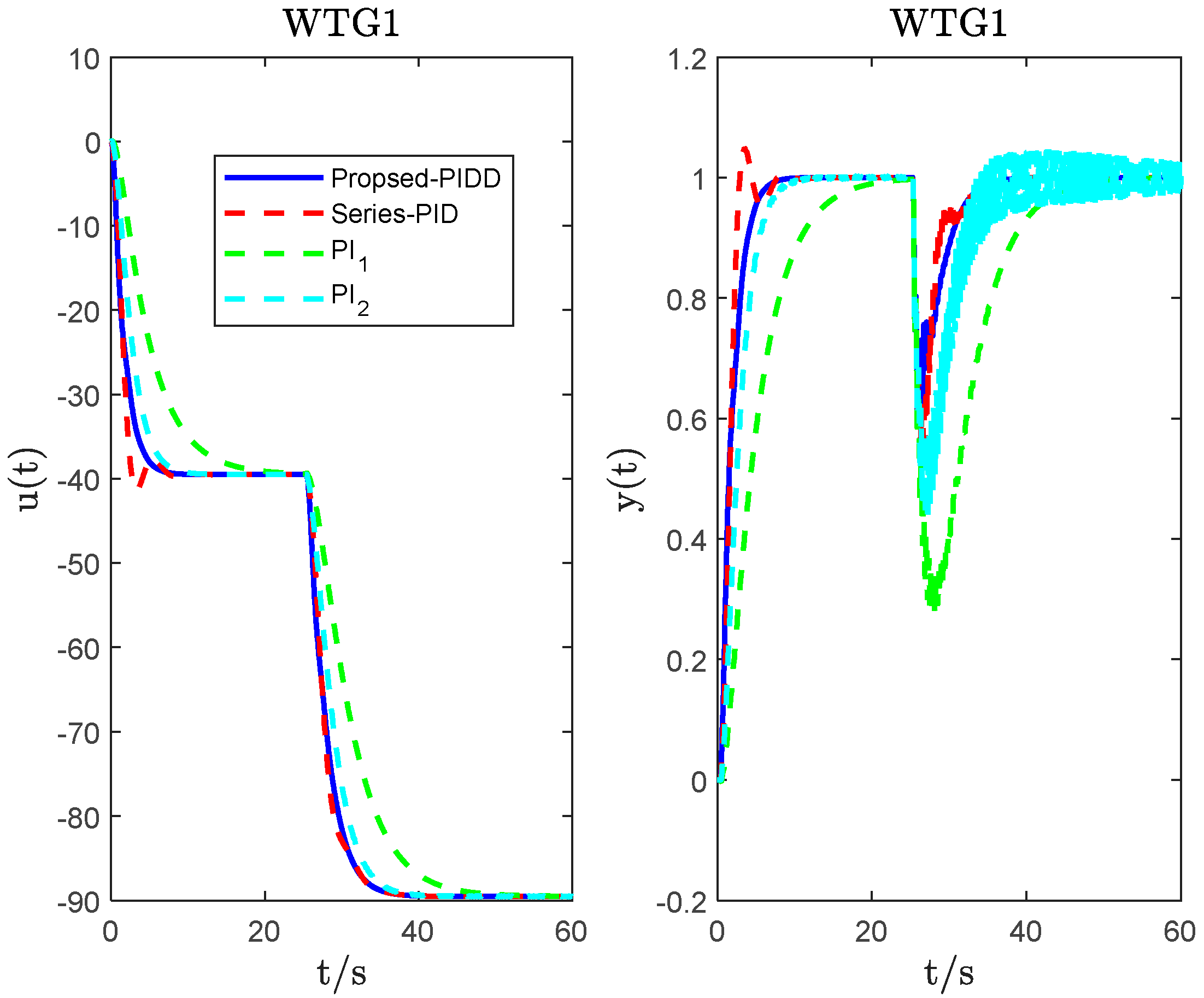
Figure 9.
The dynamic response of the WTG1 system under step disturbance when increases by 10%.
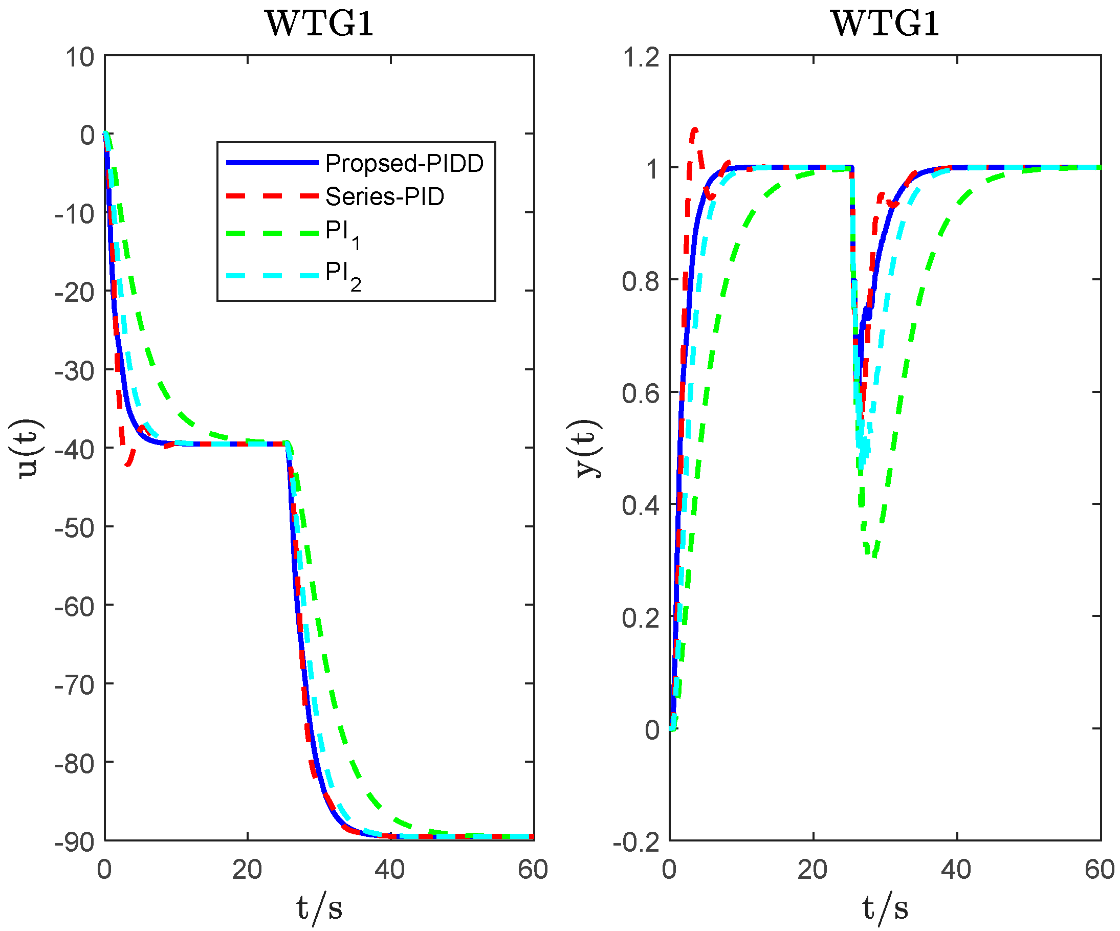
Figure 10.
The dynamic response of the WTG2 system: the controller output dynamic step responses (the left); the system output dynamic step responses (the right).
Figure 10.
The dynamic response of the WTG2 system: the controller output dynamic step responses (the left); the system output dynamic step responses (the right).

Figure 11.
The dynamic response of the WTG2 system under step disturbance: the controller output dynamic step disturbance responses (on the left); the system output dynamic step disturbance responses (on the right).
Figure 11.
The dynamic response of the WTG2 system under step disturbance: the controller output dynamic step disturbance responses (on the left); the system output dynamic step disturbance responses (on the right).

Figure 12.
The dynamic response of the WTG2 system with noise: the controller output noise responses (on the left); the system output noise responses (on the right).
Figure 12.
The dynamic response of the WTG2 system with noise: the controller output noise responses (on the left); the system output noise responses (on the right).
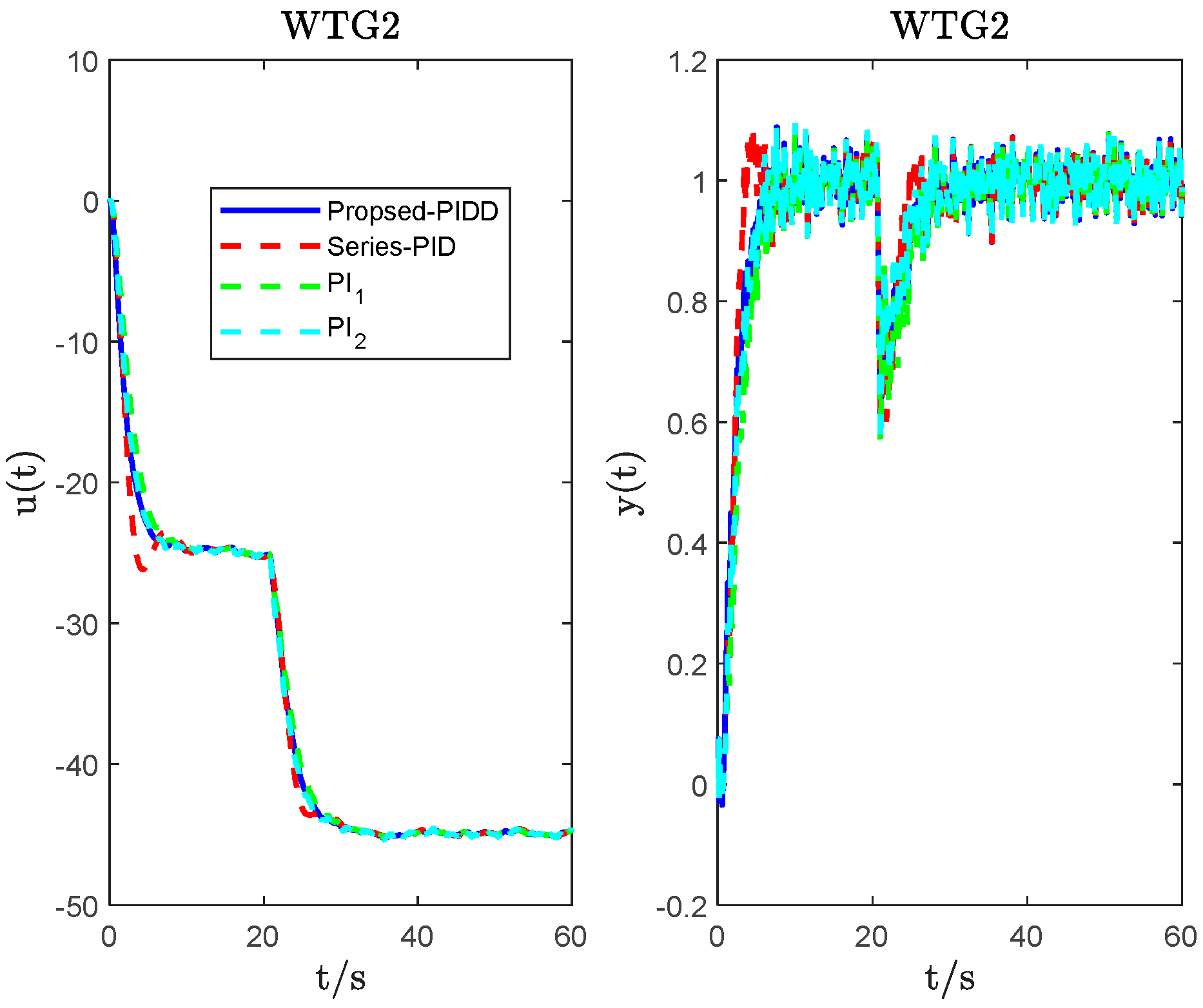
Figure 13.
The robustness change process of different methods for WTG2.

Figure 14.
The dynamic response of the WTG2 system under step disturbance when decreases by 10%.
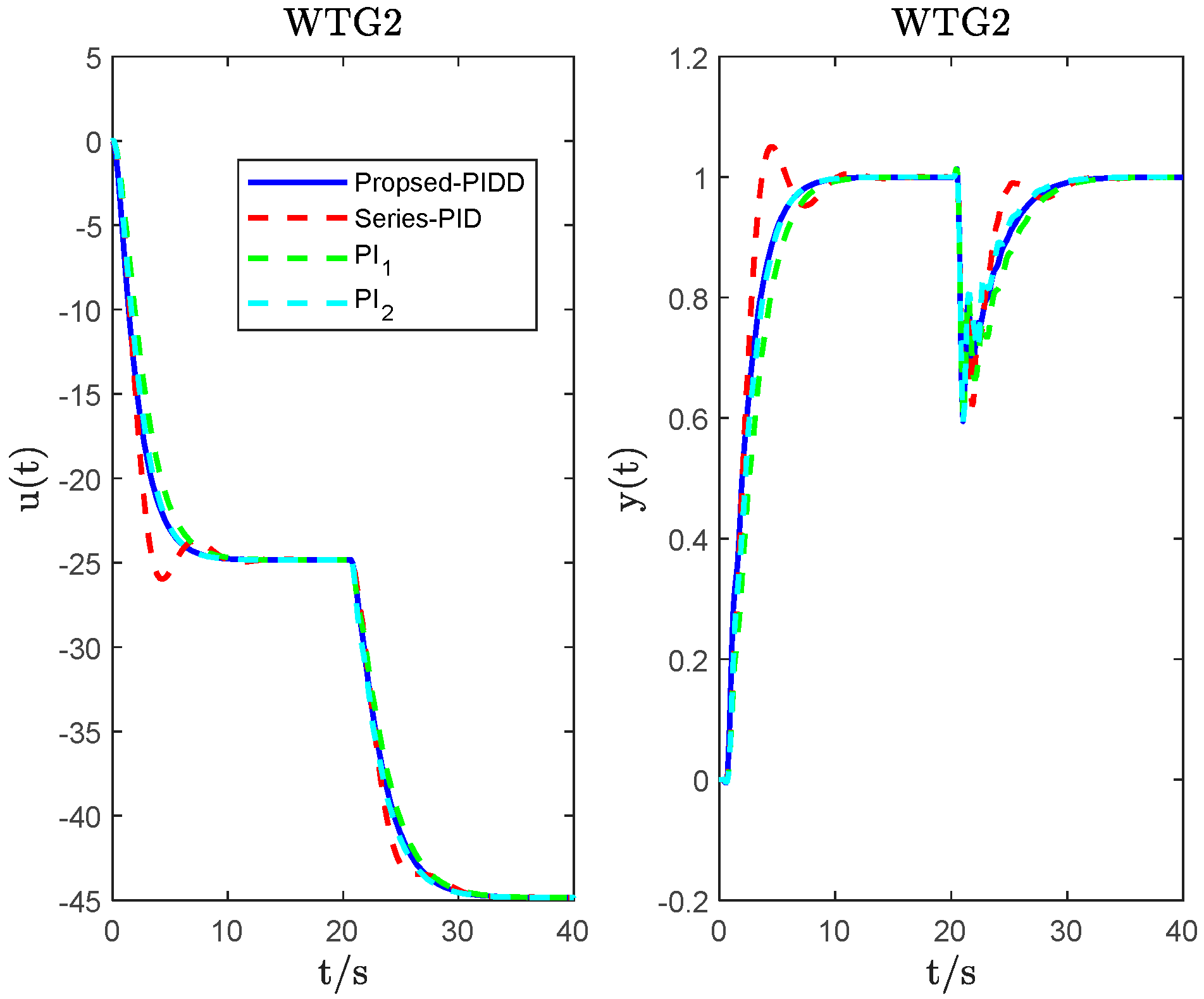
Figure 15.
The dynamic response of the WTG2 system under step disturbance when increases by 10%.
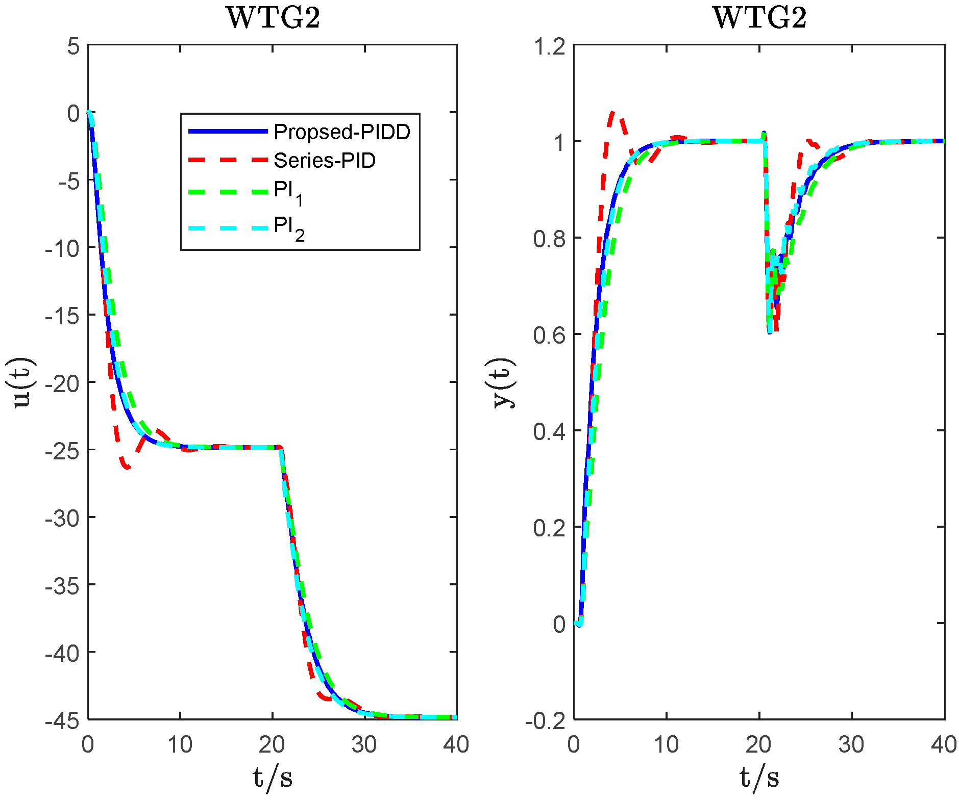
Figure 16.
Bode plots of WTG1, WTG2 and WTG3.
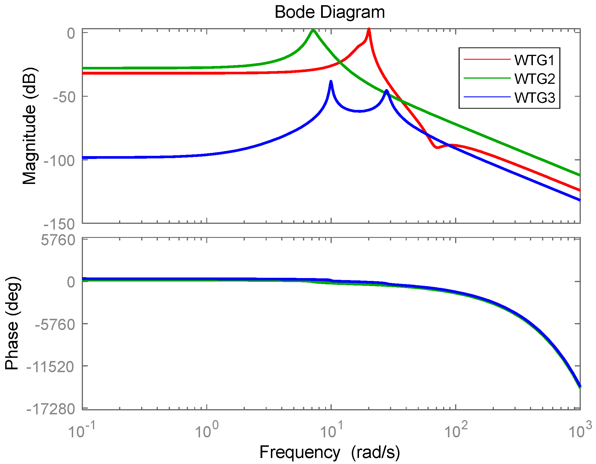
Figure 17.
The dynamic response of the WTG3 system: the controller output dynamic step responses (on the left); the system output dynamic step responses (on the right).
Figure 17.
The dynamic response of the WTG3 system: the controller output dynamic step responses (on the left); the system output dynamic step responses (on the right).
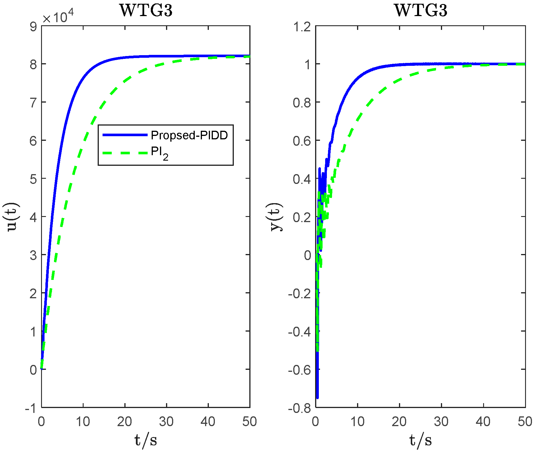
Figure 18.
The dynamic response of the WTG3 system under step disturbance: the controller output dynamic step disturbance responses (on the left); the system output dynamic step disturbance responses (on the right).
Figure 18.
The dynamic response of the WTG3 system under step disturbance: the controller output dynamic step disturbance responses (on the left); the system output dynamic step disturbance responses (on the right).
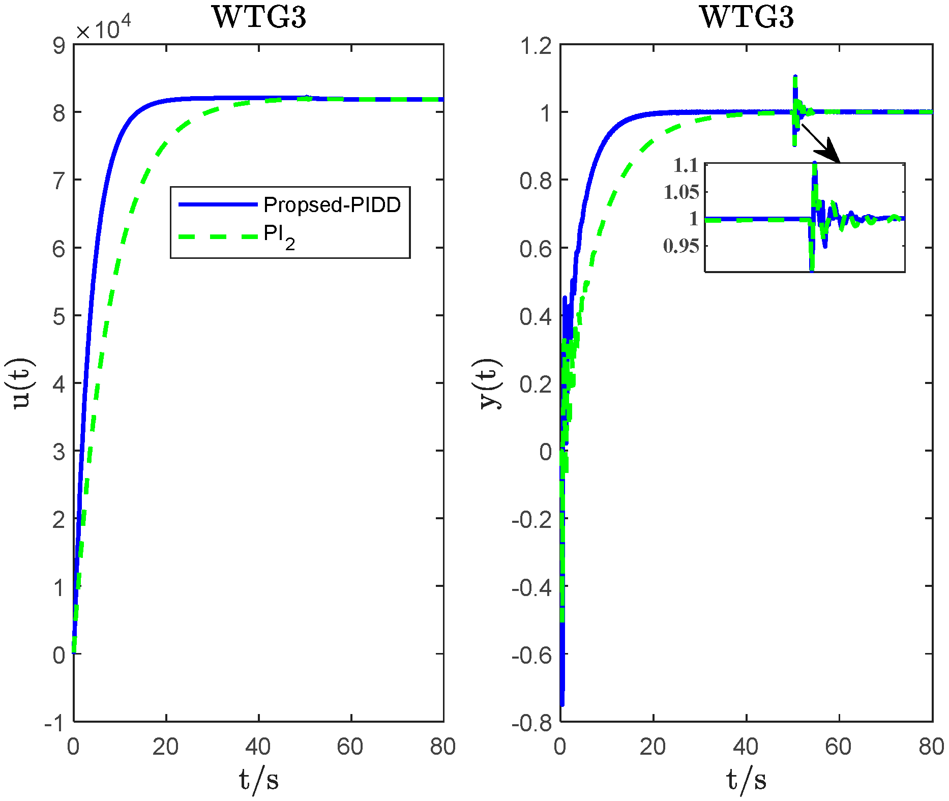
Figure 19.
The dynamic response of the WTG3 system with noise: the controller output noise responses (on the left); the system output noise responses (on the right).
Figure 19.
The dynamic response of the WTG3 system with noise: the controller output noise responses (on the left); the system output noise responses (on the right).
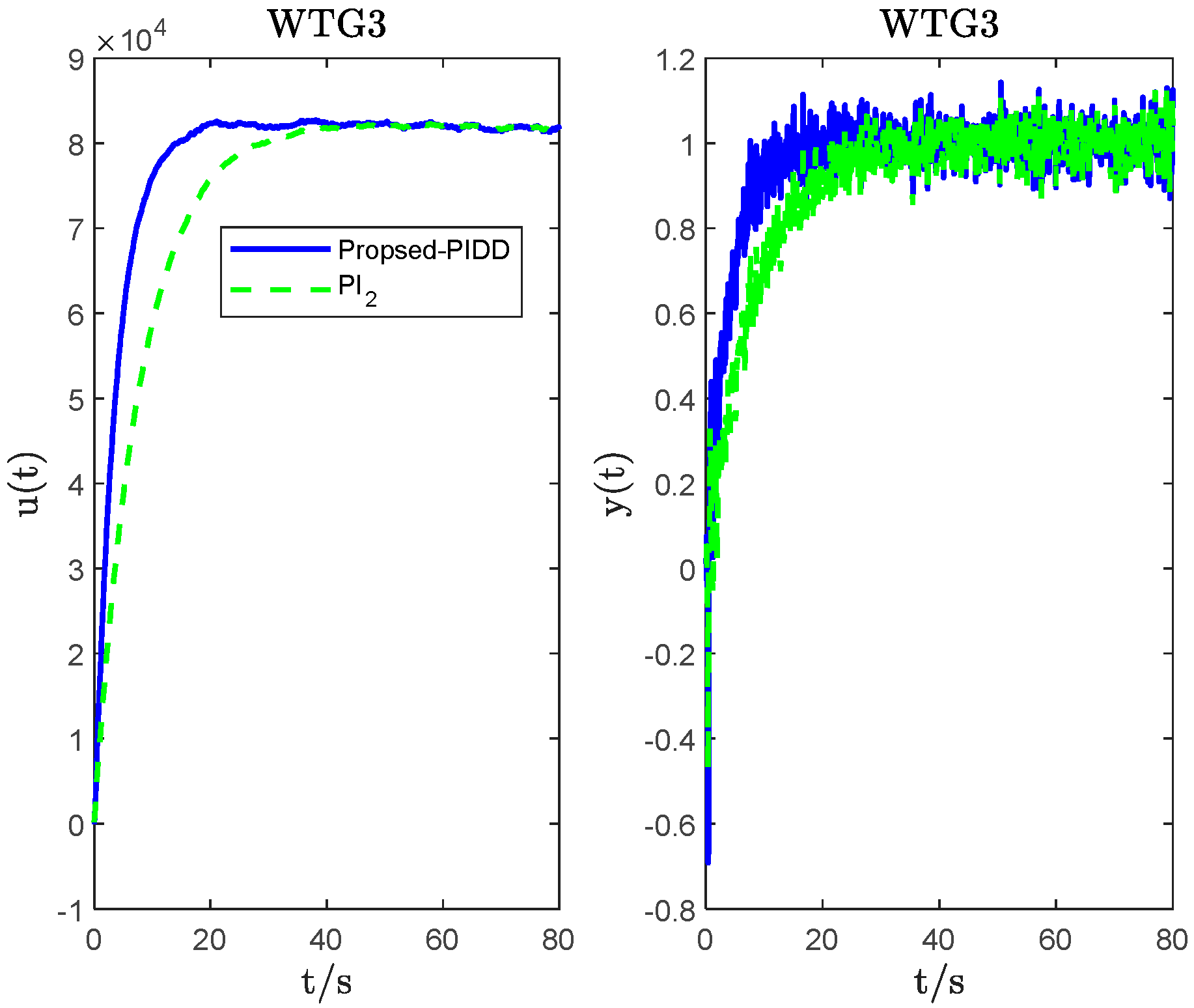
Figure 20.
The robustness change process of different methods for WTG3.
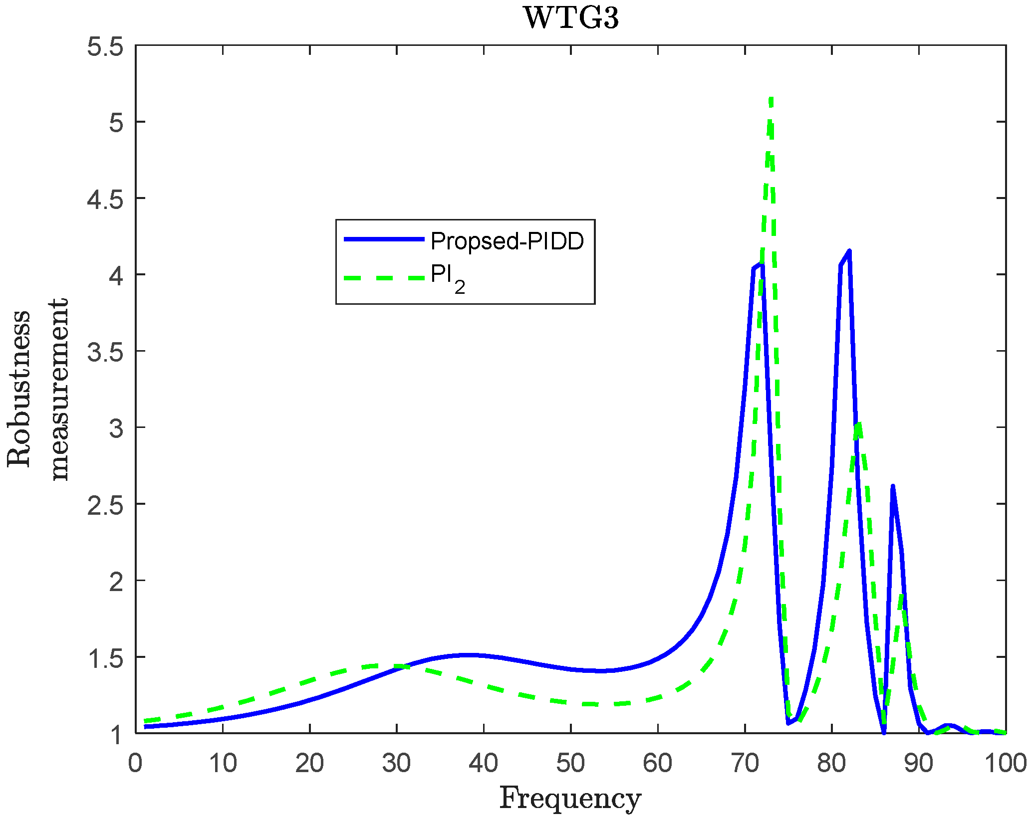
Figure 21.
The dynamic response of the WTG3 system under step disturbance when decreases by 10%.
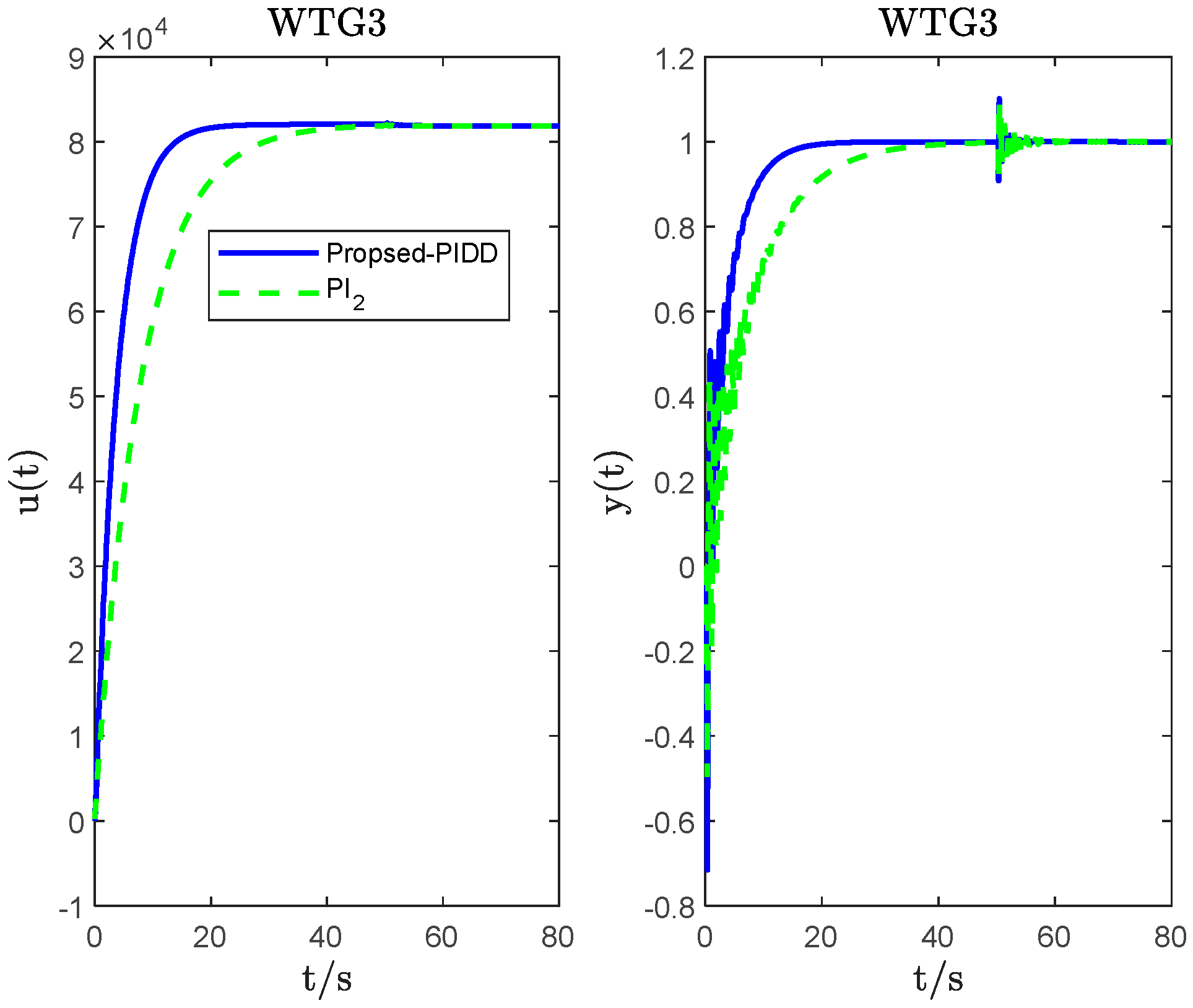
Figure 22.
The dynamic response of the WTG3 system under step disturbance when increases by 10%.

Table 1.
Parameters of Equation (1).
| Process/Parameters | ||||||||
|---|---|---|---|---|---|---|---|---|
| WTG1 | −0.6219 | −8.7165 | −2911 | 5.018 | 691.3 | 1949 | 1.15 × 10⁵ | 0.25 |
| WTG2 | 2.426 | −4.6345 | −147.3 | 4.857 | 126.2 | 266.4 | 3.66 × 10³ | 0.25 |
| WTG3 | −0.2545 | −0.0647 | 0.9384 | 2.28 | 878.5 | 437.7 | 7.7 × 10⁴ | 0.25 |
Table 2.
Parameters of Equation (2).
| Process/Model | |||||
|---|---|---|---|---|---|
| WTG1 | −0.0253 | 0.05 | 0.10 | 0.018 | 0.42 |
| WTG2 | −0.0402 | 0.14 | 0.42 | 0.060 | 0.51 |
| WTG3 | 1.2374 × 10⁻⁵ | 0.1006 | −3.5159 | 0.0157 | 0.10 |
Table 3.
Parameters and performance metrics of the different methods for WTG1.
| System | Methods | Controller Parameters | Robustness Index | ITAE Index | Total Variation | ||||
|---|---|---|---|---|---|---|---|---|---|
| ITAE | TV | ||||||||
| WTG1 | PIDD2 ( = 0.1; = 0.03) | 3.0986 | −52.3634 | 1.3377 | −0.1854 | 3 | 2.9583 | 4.20 × 10³ | 102.4039 |
| Series_PID | −28.46 | −39.5278 | −20.4912 | 4.4391 | 4.60 × 10³ | 107.545 | |||
| PI1 | 1 | −9 | 2.827 | 2.10 × 10⁴ | 91.5393 | ||||
| PI2 | 1.0242 | −20.5914 | 6.0392 | 8.00 × 10³ | 91.868 | ||||
Table 4.
Parameters and performance metrics of the different methods for WTG2.
| System | Methods | Controller Parameters | Robustness Index | ITAE Index | Total Variation | ||||
|---|---|---|---|---|---|---|---|---|---|
| ITAE | TV | ||||||||
| WTG2 | PIDD2 ( = 0.1; = 0.15) | 10.9016 | −32.8347 | −4.2875 | 1.7644 | 1.8 | 2.0181 | 3.30 × 10³ | 44.9046 |
| Series_PID | −20.73 | −20.73 | −20.73 | 3.2589 | 3.50 × 10³ | 56.4178 | |||
| PI1 | 0.5 | −15 | 2.6708 | 4.00 × 10³ | 45.9361 | ||||
| PI2 | 1 | −20 | 3.4635 | 3.00 × 10³ | 47.4178 | ||||
Table 5.
Parameters and performance metrics of the different methods for WTG3.
| System | Methods | Controller Parameters | Robustness Index | ITAE Index | Total Variation | ||||
|---|---|---|---|---|---|---|---|---|---|
| ITAE | TV | ||||||||
| WTG3 | PIDD2 ( = 0.55; = 0.055) | −146.50 | 1.6787 × 10⁴ | −6.7989 | 1.2153 | 8 | 4.1550 | 14.2170 | 89.7097 |
| PI2 | 250 | 10,000 | 5.1587 | 31.3843 | 89.8783 | ||||
Disclaimer/Publisher’s Note: The statements, opinions and data contained in all publications are solely those of the individual author(s) and contributor(s) and not of MDPI and/or the editor(s). MDPI and/or the editor(s) disclaim responsibility for any injury to people or property resulting from any ideas, methods, instructions or products referred to in the content. |
© 2023 by the authors. Licensee MDPI, Basel, Switzerland. This article is an open access article distributed under the terms and conditions of the Creative Commons Attribution (CC BY) license (https://creativecommons.org/licenses/by/4.0/).
Share and Cite
MDPI and ACS Style
Hu, X.; Tan, W.; Hou, G. PIDD2 Control of Large Wind Turbines’ Pitch Angle. Energies 2023, 16, 5096. https://doi.org/10.3390/en16135096
AMA Style
Hu X, Tan W, Hou G. PIDD2 Control of Large Wind Turbines’ Pitch Angle. Energies. 2023; 16(13):5096. https://doi.org/10.3390/en16135096
Chicago/Turabian StyleHu, Xingqi, Wen Tan, and Guolian Hou. 2023. "PIDD2 Control of Large Wind Turbines’ Pitch Angle" Energies 16, no. 13: 5096. https://doi.org/10.3390/en16135096
Note that from the first issue of 2016, this journal uses article numbers instead of page numbers. See further details here.