
A 3D Transient CFD Simulation of a Multi-Tubular Reactor for Power to Gas Applications


1
Carbon and Catalysis Laboratory (CarboCat), Department of Chemical Engineering, Faculty of Engineering, Universidad de Concepción, P.O. Box 160-C, Concepcion 4070386, Chile
2
Environmental Engineering Department, Faculty of Environmental Sciences and EULA Chile Centre, Universidad de Concepción, P.O. Box 160-C, Concepcion 4070386, Chile
*
Author to whom correspondence should be addressed.
Energies 2022, 15(9), 3383; https://doi.org/10.3390/en15093383
Submission received: 20 March 2022
/
Revised: 19 April 2022
/
Accepted: 24 April 2022
/
Published: 6 May 2022
(This article belongs to the Special Issue Advances in Power-to-X Technologies Using Biogas as Carbon Source)
Abstract
:A 3D stationary CFD study was conducted in our previous work, resulting in a novel reactor design methodology oriented to upgrading biogas through CO2 methanation. To enhance our design methodology incorporating relevant power to gas operational conditions, a novel transient 3D CFD modelling methodology is employed to simulate the effect of relevant dynamic disruptions on the behaviour of a tubular fixed bed reactor for biogas upgrading. Unlike 1D/2D models, this contribution implements a full 3D shell cooled methanation reactor considering real-world operational conditions. The reactor’s behaviour was analysed considering the hot-spot temperature and the outlet CH4 mole fraction as the main performance parameters. The reactor start-up and shutdown times were estimated at 330 s and 130 s, respectively. As expected, inlet feed and temperature disruptions prompted “wrong-way” behaviours. A 30 s H2 feed interruption gave rise to a transient low-temperature hot spot, which dissipated after 60 s H2 feed was resumed. A 20 K rise in the inlet temperature (523–543 K) triggered a transient low-temperature hot spot (879 to 850 K). On the contrary, a 20 K inlet temperature drop resulted in a transient high-temperature hot spot (879 to 923 K), which exposed the catalyst to its maximum operational temperature. The maximum idle time, which allowed for a warm start of the reactor, was estimated at three hours in the absence of heat sources. No significant impacts were found on the product gas quality (% CH4) under the considered disruptions. Unlike typical 1D/2D simulation works, a 3D model allowed to identify the relevant design issues like the impact of hot-spot displacement on the reactor cooling efficiency.
1. Introduction
Renewable energy development is significantly hindered by the uncontrollable intermittence of most renewable resources and the unfeasibility of electricity storage. In this scenario, mass conversion of electrical power in the form of methane and/or hydrogen (power to gas) stands out as a potential solution to balance the electrical grids while at the same time offering an alternative for CO2 valorisation if the Sabatier reaction Equation (1) is used for this purpose [1]. However, the high exothermicity of this reaction severely hinders the development of this technology on an industrial scale. Consequently the design of heat removal/cooling systems remains a priority to further develop methanation reactors at the pilot and industrial scale.
The increasing interest in the development of methanation pilot plants [2,3] encourages the need for new models and designs capable of dealing with the operational challenges inherent to power to gas conditions.
While the reviewed literature expresses a special interest in fixed-bed tubular models (for their simplicity and technological readiness [4]), a lack of insight regarding a comprehensive 3D simulation of a tubular methanation reactor under PtG conditions exists. 3D simulations remain the unique alternative to understanding how a reactor model behaves in close to real-world conditions. On the contrary, current research works mainly focus on 1D single tube simplified reactors. Although they remain acceptable for process-focused studies [5,6], 3D models have proven necessary for designing industrial-sized reactors [7,8]. According to the authors’ knowledge, no current research addressed a 3D transient reactor simulation for biogas upgrading. One of the main drawbacks of simplified models is the absence of insight regarding the interaction of heat transfer mechanisms (coolant flow) and reaction engineering. Unlike transient 1D models, which incorporate heat transfer phenomena through constant heat transfer coefficients, in this work, we consider a close to real-world modelling scenario by combining both flow dynamics and chemical kinetics into a single CFD model. Our previous research [4] demonstrated the relevance of considering a turbulent model to characterise the shell-side flow since heat transfer coefficients are not constant across the tube length. Although transient 1D models remain the standard for chemical reaction engineering issues like controlling the reaction exothermicity, important design features remain obscure for such models, where coolant flow dynamics are simplified [9] or replaced by constant heat transfer coefficients [10].
In our previous work [11], a 3D stationary CFD study was conducted, resulting in a novel reactor design methodology oriented to the upgrade of biogas through CO2 methanation, Figure 1. CFD simulations were focused on coolant flow dynamics and heat transfer performance in the reactor. Therefore, the reactor’s interaction with auxiliary equipment (e.g., compressors, separators) was not considered.
A disk and doughnut arrangement was selected for its advantages over traditional reactor arrangements. Due to the axisymmetric nature of the design, all tubes are subjected to the same flow and thermal conditions. In addition, an optimal baffle disposition allows for an optimal heat transfer performance at the hot spot position due to direct exposure to the incoming coolant stream. Finally, an optimal cooling flow was identified, which minimised the pumping energy requirement while maximising heat transfer in key areas.
To enhance our design methodology incorporating relevant power to gas operational conditions, a novel transient 3D CFD modelling methodology is employed to simulate the effect of relevant dynamic disruptions on the behaviour of a tubular fixed bed reactor for biogas upgrading. The reactor’s behaviour was analysed considering the hot-spot temperature and the outlet CH4 mole fraction as main performance parameters. According to reviewed literature, dynamic operation of fixed bed methanation reactors occurs by disruptions in the inlet temperature [12,13], flow rate [10] and composition [14]. In this work, due to the relevance of composition variation in the power to gas context, a disturbance of H2 content in the inlet feed was considered, in addition, to temperature changes in the inlet stream. Finally, reactor start-up and shutdown times were determined alongside the maximum idle time (no coolant nor gas flow), which allowed for a warm start (i.e., condition in which the reactor and the coolant temperature allow for the reaction to ignite, without the need to change the design operational conditions substantially). It is expected that the present contribution will be useful for designers and engineers, providing a good reference in the field of biogas upgrade through CO2 methanation.
2. Materials and Methods
2.1. Reactor Model Description
A twenty-tube fixed bed reactor 3D model for biogas upgrade into SNG (Synthetic Natural Gas) quality was considered as the study object of the present work. Additional parameters and full reactor description can be found in [11]. According to our previous research, two reactor modules of 1 m and 0.5 m and an intermediate condensation step are required to upgrade biogas to a SNG quality gas: 97.8 mol % CH4, 0.42% CO2, 1.68% H2. This considers that the first module attains a product composition (on a dry basis) of: 90.2% CH4, 2% CO2 and 7.8% H2. Feed composition of the biogas stream should comply with the following minimum standard: 64% CH4, 32.5% CO2, 2.5% H2O and no sulphur. In addition, a H2/CO2 of 3.8 was adopted due to the difficulty of meeting the minimum H2 content in the product gas. For the sake of simplicity, only the first module was simulated, considering that the most relevant phenomena occurred in the initial sections of the reactor. Figure 2 show the entire first reactor module as simulated in the present work.
CO2 methanation kinetics Equations (2)–(5) proposed by Koschany et al. [15] was incorporated into the CFD model by means of a UDF written in C language. Kinetic parameters were adopted from [5]. A commercial Ni-based catalyst (923 K maximum operational temperature) [16] was considered. The reactor is assumed to be fully insulated by a 50 mm mineral wool layer. Table 1 summarises the base case operational conditions and reactor technical specifications.
The proposed design is modular and suitable for decentralised biogas producing plants ≈ 150 Nm3 (biogas production). Operational conditions (pressure, stoichiometric molar ratio, reaction temperature, reactor dimensions) relates to optimal values determined in our previous work based on the relevant literature review. Table 2 compares our design with previous biogas methanation simulation/experimental works. Only industrial relevant reactors were considered for comparison purposes.
2.2. Governing Equations
In this work, the unsteady form of the conservation laws of mass, energy and momentum Equations (6)–(13) in addition to the constitutive equations for the turbulence model (shell side), chemical kinetics (tubes), thermal model (tubes) and momentum exchange (tubes) were adapted from the steady-state conservation laws documented in detail in our previous work and detailed in Table 3.
2.3. Numerical Methods
The SIMPLE algorithm was applied to couple the pressure and velocity equations. Discretisation schemes for momentum, energy and species were of the second-order upwind, while a standard approach was selected for the pressure equation. The temporal term was discretised with the first-order implicit formulation. The least-squares cell-based scheme was chosen to discretise variable gradients. Under-relaxation factors of 0.6 were considered for momentum and balance equations, while energy and species were set at 0.4. Wall y+ value was monitored for the coolant flow to guarantee standard wall function requirements (y+ > 30) and ensure an accurate approach for heat transfer coefficients estimation on tube walls. In addition, the maximum cell convective Courant number (≈20–40) was monitored inside the reactive tubes to confirm the suitability of the transient formulation (time step and max iterations per time step). A time step of 1 s complies with the convective Courant number requirements; however, in this work, a time step of 0.5 s was used to represent better the transient phenomena. Steady-state was verified through the following relevant variables: CO2 and CH4 mole fraction at the tube’s outlet and maximum (hot-spot) temperature. Unsteady governing equations were discretised and solved using the CFD code ANSYS Fluent by the finite volume method.
2.4. Physical Models and Boundary Conditions
Figure 2 illustrates the reactor physical model and the implemented boundary conditions. The CFD model comprised three distinct cell zones (domains): (1) coolant (fluid), (2) tubes (porous media) and (3) baffles (solid). For a detailed description of the thermophysical properties in each cell zone, refer to Appendix A. A velocity inlet (4) of 0.5 m/s was utilised for the coolant inlet, equivalent to 3.5 m3/h of coolant flow at 523 K. Gas feed at tube inlets (5) was characterised by a mass flow inlet of 2.15 × 10⁻⁴ kg/s (≈30 Nm3/h). In order to calculate the pressure drop across reactive tubes and shell sides, a zero static pressure condition was set at both outlets, tubes (6) and coolant (7). In addition, operating pressure was set at 1 and 10 bar for coolant and reactive tubes, respectively. Heat transfer surfaces (tube to coolant, baffle to coolant) were defined through thermal coupled walls (8). The reactor is assumed to be fully encapsulated in mineral wool insulation. A convective heat transfer coefficient of 5 W·m2·K−1 [26] and a free stream temperature of 300 K to simulate heat loss to the environment were adopted at the reactor outer walls (9). Table 4 summarises the boundary and cell zone conditions used to set the CFD model.
2.5. Meshing Approach
Figure 3 illustrates the reactor mesh across all sub-domains. Ansys Design Modeller and Ansys Meshing were used for domain and mesh preparation in this work. A non-conformal dual meshing approach was adopted. A tetrahedral mesh (1) was chosen for the coolant (fluid) domain due to its capacity to easily conform to restrictive geometries. According to standard wall function requirements, inflation layers were created (2) at coolant-tube walls to guarantee a Y+ value of 30. A hexahedral grid (3) was used on all tubes (porous media domain) to maximise mesh quality in areas where a chemical reaction occurs. A coarser hexahedral mesh was considered in both disk (4) and doughnut (5) types regarding solid baffles. Non-conformal interface zones were created to connect thermally coupled zones (i.e., when solid (6) and porous media (7) cell zones match the fluid domain). Table 5 summarises mesh quality details for each reactor’s model sub-domains. Our previous work checked Mesh independence by calculating the average temperature at the tube’s outlet and the average CO2 mole fraction at the tube’s outlet under a steady state.
2.6. CFD Model Validation
The present 3D CFD model was validated in a twofold manner in our previous work [11]. First, the chemical reaction model was validated against steady-state experimental data from [16], considering a CO2 methanation reactor of similar size (1 m in length, 30 mm in diameter). Secondly, the Gnielinski correlation [27] was used to validate the heat transfer coefficients for the tube to coolant interface. Benchmark simulation results agreed well with both experimental and correlation data. The hot spot position was accurately predicted with a 5% error in the axial coordinate. The predicted axial temperature profile showed a maximum error of 8.5% against experimental data, while numerically calculated heat transfer coefficients revealed a maximum deviation of 20% against the Gnielinski correlation. We used the same geometrical configuration and mesh from our previous work in this work. In addition, the optimal operational conditions found in [11] were adopted as the basis for all the transient simulations performed in the present work. Thus, preserving the validity of chemical kinetics and heat transfer models.
2.7. Reactor Dynamic Operation
In this work, dynamic simulations were conducted to characterise three relevant scenarios. Firstly, start-up and shutdown times were determined under nominal conditions. Secondly, the reactor was subjected to relevant dynamic disruptions, namely H2 feed interruption and changes in the inlet temperature. Finally, the maximum reactor “standby time” (no coolant and gas feed), which allows for a warm start, was determined.
2.7.1. Start-Up and Shutdown
Firstly, a “only biogas run” was performed, where no H2 was injected so that the flow field inside tubes (only biogas) and coolant side becomes uniform (non-reactive steady-state). In a second step, H2 injection begins until an ignited steady state is reached (reactor start-up). This start-up operation is characterised by the operational conditions detailed in Table 1. Since the feed is rich in methane, no additional measures (e.g., catalyst dilution) for thermal control were considered. Finally, the reactor shutdown is simulated, interrupting the H2 feed while maintaining the flow of biogas at operational temperature. The simulation sequence summarises as follows:
- Non-reactive steady state: Biogas and coolant under nominal operational conditions are injected until a fully developed flow is attained. A steady-state simulation was conducted to simulate the abovementioned flow and used as an initial condition in further transient studies.
- Reactor start-up: As H2 supply begins, reactor steady state was checked by monitoring the following variables: average CO2 mole fraction, maximum temperature, average temperature and CH4 mole fraction at the tube outlet. A change of less than 1 × 10⁻⁴ for all monitored variables in two successive time steps was considered as proof of steady-state condition.
- Reactor shutdown: As a steady state was reached, H2 supply was interrupted. Pure biogas (at 523 K) was fed to the reactor until the average tube temperature matched the coolant temperature (523 K). The average gas composition inside tubes reached that of pure biogas. Biogas is assumed to be continuously recirculated to the bio-digestor under reactor shutdown operation.
2.7.2. Dynamic Disruptions
As mentioned, the impact of dynamic disruptions on the reactor was numerically simulated through inlet composition and temperature disruptions. After a steady state was attained, the H2 supply was interrupted. Then, pure biogas (at reaction temperature) was injected into the reactor for 30 s (according to the European Union guidelines for electricity transmission [28], in case of frequency disruption in the grid, the transmission system operators (TSO) shall restore the reference value at the latest after 30 s. Therefore a 30 s H2 feed interruption was considered to depict a relevant electricity supply disruption) while preserving the GHSV (same superficial velocity). Then H2 injection is resumed. On the other hand, temperature perturbations were considered through a ±20 K variation in the feed gas. Special attention is given to temperature disruptions due to their relevance in triggering “Wrong Way” behaviour [12]. All simulations were conducted until steady state conditions were observed.
2.7.3. Stand by Reactor
To determine the maximum “standby” of a non-feed and non-coolant flow condition, the reactor cooling process was simulated in the absence of heating sources. After the reactor shutdown, both coolant and biogas inflows are interrupted. This simulation aimed to determine the maximum reactor idle time, allowing for the reactor’s resumption (warm start) with no necessity of heating the inflow gases beyond the optimal temperature (523 K).
3. Results and Discussion
3.1. Reactor Start-Up and Shutdown Simulation
First, the reactor model simulates the start-up process as detailed in Section 2.7.1. In this study, CFD simulations were oriented towards identifying temperature contours in the hot spot affected area since it strongly influences the reactor operational flexibility. Additionally, the CH4 mole fraction at the reactor outlet was given special attention for its relevance to the product gas quality. Progress towards the steady state was simulated considering nominal operational conditions of the reactor. At t = 0 s, reactor feed is adjusted from pure biogas to a mixture of biogas and H2, preserving a stoichiometric ratio of 3.8. The volumetric flow remains constant in both conditions (same GHSV). According to Figure 4a) the reactor needs 70 s to reach the maximum temperature after H2 injection. A steady-state hot spot is observed after 330 s from H2 injection. A maximum temperature of 879 K is reached, which means that it is possible to maintain a safe and stable start-up operation in the reactor under the considered operational conditions without diluting the catalytic bed or the addition of complex cooling and control systems. During this transient operation, it is assumed that no flow is directed to the second methanation module. Shutdown operation was also simulated, and the reactor thermal behaviour was characterised. After the reactor reaches the steady state (330 s), H2 feed is interrupted, and pure biogas (523 K) injection is resumed. The reactor assumes a “non-reactive” flow mode aimed at maintaining warm start conditions in the absence of chemical reaction.
Figure 5 illustrates the temperature contours in the characteristic reactor tube at different time series: 10 s, 20 s, 40 s, 330 s. As typical in exothermic reactions, a distinct hot spot appears at the reactor’s inlet. High reactant concentration results in higher reaction rates and large temperature gradients. A fully developed hot spot is observed at 330 s. Due to heat removal and viscosity effects, a large temperature gradient (≈200 K) exists radially at the hot spot. Downstream to the hot-spot affected area, a low-temperature zone appears, where the reactor matches the coolant temperature (523 K). As it is common in fixed bed reactors, it should be noted that most of the extent of reaction takes place in the first ≈250 mm of the reactor’s first module. As already mentioned in our previous work, the extent of reaction is mostly driven by kinetic effects in this section. Downstream, it becomes increasingly difficult to reach higher conversions unless the thermodynamic equilibrium is shifted back to products (e.g., water removal). As detailed in our previous work, interstage water removal becomes mandatory to achieve the required SNG quality. As Figure 4b) shows, after ≈130 s of hydrogen feed interruption, the hot spot affected area cools down to the ignition temperature. From the CFD simulations, it can be concluded that nearly six minutes (330 s) are needed for the reactor’s first module to reach a steady state (start-up operation). In contrast, the reactor’s first module requires two minutes to attain warm start conditions after H2 is interrupted (shutdown operation). Reported start-up times in similar simulation and experimental works range in the minutes for all cases. Bremer [29] reported 1000 s to reach a steady state for a 20 mm × 5 m, 720 h−1 GHSV tubular reactor. Fache [30] determined optimal operational variables for a multi-tubular reactor with staged dilution. An optimal start-up time of 178 s was found for a total flow of 0.44 m3/h per reactor tube. Matthischke [5] determined the start-up times for an adiabatic and a cooled tubular reactor. The latter needed 200 s to attain a steady temperature profile while the former required 400 s. Dannesboe [25] developed a pilot plant scale double pass reactor with boiling water cooling for a 10 Nm3/h biogas flow. Steady state operation, with respect to the temperature profile, was achieved after 25 min. Giglio [6] proposed a three-staged methanation unit with two water removal steps. A product gas with a 95% methane content was obtained after 130 s from a warm start.
3.2. Reactor Response to H2 Feed Interruption
The first disturbance was simulated as a step-change in the inlet gas composition due to a sudden loss of the H2 feed from the electrolyser for 30 s. The reactor response was followed from this reference state, t = 360 s (330 s “steady state” +30 s interruption) to the recovery of steady-state behaviour after 450 s from the reactor’s start-up. Figure 6a represents the reactor temperature contours after 30 s the H2 feed was disrupted. Due to the cooling effect of the inlet biogas stream and the absence of H2, the original hot spot dissipates, but a high-temperature zone persists downwards. As H2 feed resumes, a new hot spot begins to form downwards, at t ≈ 375 s Figure 7, due to the displacement of the maximum temperature zone, Figure 6b.
As a new hot-spot forms, the temperature rises near the reactor inlet, Figure 6c prompting the resurgence of the original hot spot after t ≈ 410, Figure 6d. As the temperature progressively increases, the reaction front moves forward until the hot spot is fully formed 90 s after the H2 feed was interrupted. This behaviour can be explained as follows: after 30 s of H2 feed interruption and biogas injection, an area downwards of the original hot spot position is not cooled enough during the 30 s of biogas injection, preserving a high-temperature zone (642–682 K) Figure 6a, due to the catalytic bed thermal inertia. As H2 injection is resumed, the concentration front reaches this high-temperature surface, triggering a transient hot spot similarly as observed by Try et al. [12]. As more reactants convert to CH4 in this area, fewer reactants become available downwards to sustain this hot spot. Consequently, the reaction front moves upwards, where a higher concentration of reactants allows for higher reaction rates and temperature. As fewer reactants reach the downstream part of the reactor, the transient hot spot, Figure 6b, dissipates. According to Figure 7, a step disruption of the H2 feed impacts the outlet CH4 composition during 90 s, i.e., (from t = 360 s to t = 450 s).
At t = 450, the steady state CH4 outlet mole composition stabilises around 0.55, allowing for the fulfilment of SNG quality requirements (90.2% CH4 on a dry basis after the first methanation module). At the same time, the low-temperature transient hot spot is entirely replaced by a high-temperature one after the 450 s (90 s after H2 resumption).
3.3. Reactor Response to Temperature Disruptions
3.3.1. 20 K Feed Temperature Rise
Figure 8 shows the temperature contours of the reactor subjected to a 20 K step-rise in the feed gas temperature (523 K–543 K). Figure 9 shows the transient response of the hot spot temperature and the CH4 mole fraction at the reactor’s outlet, respectively. The inlet temperature rise triggered a transient drop in the reactor hot spot temperature from t = 0 to t = 25, Figure 9. Similar behaviour was observed by Li et al. [13] for a sudden temperature rise (523 K to 543 K) in an adiabatic CO methanation reactor. Higher upstream temperatures prompted higher reaction rates and CO2 consumption near the reactor inlet, Figure 10. As the concentration front moves upwards, Figure 10 shows fewer reactants remain available downstream. Consequently, the reactor undergoes a transient drop in the maximum temperature, Figure 8a,b. At approximately t = 25 s from the disruption, in Figure 9, the hot spot attains its minimum temperature (850 K), after which it begins to rise until it reaches 892 K at t = 40 s Figure 9. After 120 s, a new steady state becomes apparent by a new maximum temperature (892 K up from 879 K) Figure 9, and the stabilisation of the concentration front upwards, Figure 10c. Regarding the CH4 formation, Figure 9, this disruption does not significantly affect the minimum outlet mole fraction required to fulfil SNG quality (>0.55). Although the hot spot moved upwards from the optimal design position (i.e., between the inlet and the first baffle), it remained in the maximum heat transfer area due to exposure to the incoming coolant stream at high velocity directly from the inlet, Figure 11.
3.3.2. 20 K Feed Temperature Drop
Figure 12 shows the temperature contours of the reactor subjected to a 20 K step-drop in the feed gas temperature (523 K–503 K). In contrast, Figure 13 shows the transient response of the hot spot temperature and the CH4 mole fraction at the reactor’s outlet, respectively. A transient hot spot of 923 K begins to appear after 20 s, Figure 12b and it is completely formed at 35 s, Figure 12c. The observed wrong way behaviour can be explained in accordance with the works of [12,13]. As the temperature diminishes in the upstream section of the reactor, the reaction rate diminishes accordingly, prompting a successive increment in the CO2 concentration near the inlet due to the movement of the reaction front towards the outlet, Figure 14. Owing to the bed’s thermal inertia, the incoming gas stream at a lower temperature (503 K) cannot cool the bed quickly enough. Therefore, the high bed temperature and the increasing reactant concentration trigger a transient “high temperature” hot spot between t = 0 s to t = 35 s, Figure 13. This transient hot spot surpassed the maximum steady-state temperature by 43 K (880 K to 923 K), exposing the reactor to its maximum operational temperature (923 K). A new steady state is attained after 200 s the disruption occurs, characterised by an 872 K hot spot Figure 12e. Finally, the wrong-way behaviour tends to disappear as the concentration front stabilises around its final position, Figure 14c, from t = 40 s onwards, Figure 13. As in Section 3.3.1, the CH4 average outlet mole fraction, Figure 13, remains under acceptable ranges to fulfil the required SNG quality (>0.55). As the hot spot moved downwards from the optimal design position (i.e., between the inlet and the first baffle), a loss in cooling effectivity occurs due to the displacement out of the optimal cooling zone, Figure 15. In this case, the high-temperature hot spot may be attributed partially to this loss of cooling effectivity during the hot spot transition.
3.4. Stand by Reactor Simulation
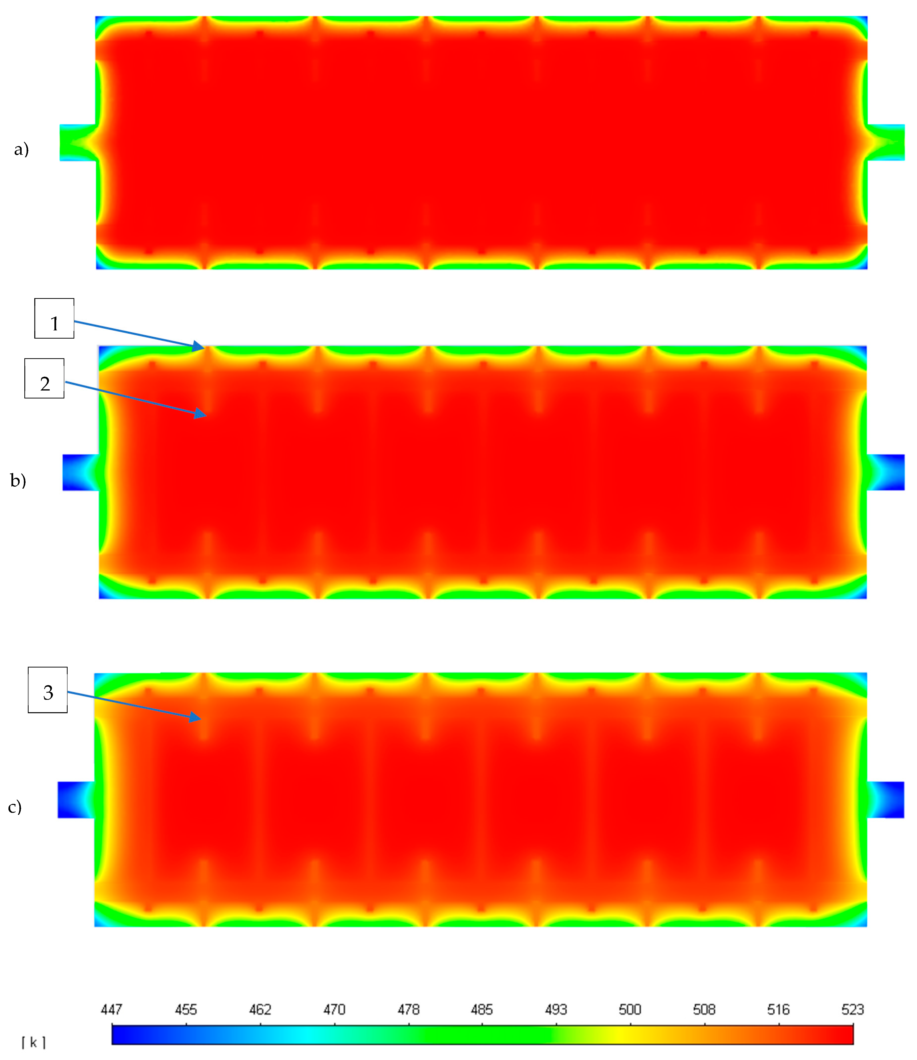
Figure 14a–c shows the YZ plane temperature contours of the reactor in standby mode after one, three, and five hours, respectively, as all external and internal heat sources were suspended (no coolant, gas flow, or reaction heat). As expected, temperature reduction is more significant in the non-insulated areas (coolant inlet and outlets) and in the reactor corners, where two heat transfer fronts exist. Due to the high thermal conductivity of the reactor baffles, a thermal bridge effect is observed from the reactor centreline to the surroundings, where the doughnut type baffle comes in contact with both the surroundings (1) and the inner section of the reactor (2). After five hours of idle time, catalytic tubes zones in contact with doughnut baffles tend to be at a lower temperature than the surroundings (3).
According to Figure 16a, after one hour of idle time, the reactor preserves a temperature of 523 K in the catalytic tubes, allowing for a warm start under optimal conditions. After three hours, the catalytic tubes mostly hold a temperature over 516 K, except in the zones where a thermal bridge exists. At this temperature, a warm start is still possible without the necessity to heat the reactants beyond 523 K or the reactor again up to 523 K. Finally, after five hours of idle time, a minimum temperature of 500 K is observed in the catalytic tubes inlets/outlets and the areas affected by thermal bridges. Although possible, a reactor warm-start is not desirable since the start-up time of the reactor will be raised, and operational parameters like CO2 conversion will be affected due to lower reaction rates, leading to a lower quality product gas. As an alternative, further heating of reactants is possible to enhance the reaction rate in low-temperature zones. However, this would demand additional control routines to keep the original operational conditions. Therefore, a maximum of 3 h of idle time is possible to allow the optimal ignition of the reactor (warm-start conditions).
4. Conclusions
A 3D fixed bed methanation model was evaluated under dynamic disruptions in this work. The main aim was to enhance our 3D methanation reactor design methodology by incorporating relevant power to gas operational elements. Firstly, the required start-up and shutdown times were determined. As a second step, dynamic perturbations were simulated through a 30 s H2 feed disruption and ±20 K temperature variation in the gas feed. Finally, the maximum idle time (no coolant or gas flow) was determined, which would allow a warm start without the need to alter the nominal operational conditions.
The reactor reached a steady state after 330 s from a warm start, in line with similar fixed bed reactor studies. On the other hand, the reactor needed 130 s to dissipate most of the reaction heat and return to nominal warm-start conditions. A 30 s H2 feed disruption showed the appearance of a transient low-temperature hot spot. At t = 450 s (90 s after the H2 feed was resumed), the maximum temperature and profile returned to the original steady-state condition. A sudden 20 K (523–543 K) rise in the inlet temperature triggered a lower temperature transient hot spot than the nominal case. On the other hand, a sudden 20 K (523–503 K) drop in the inlet stream led to higher transient temperatures. As a result, a high-temperature hot spot (≈923 K) was generated, which exposed the catalyst to its maximum operating temperature. According to simulation results, inlet temperature disruptions did not affect the minimum CH4 outlet mole fraction. However, in the case of a 30 s H2 feed loss, 90 s were necessary to stabilise the outlet concentration around 0.55. The appearance of wrong way behaviour was explained by moving concentration fronts prompted by a combination of transient reactant concentration and thermal inertia of the bed. Finally, in the absence of all heat sources, the reactor maintained warm start conditions for 3 h of idle operation. Further increment in the idle time could be attained at the expense of an increment in the reactor insulation layer.
The present contribution probed the significance of a 3D CFD model in designing tubular reactors subjected to dynamic disruptions. Unlike 1D/2D based simulation works, a 3D model allows identifying relevant design issues like the effect of different hot spot positions on the reactor cooling capability. Moreover, the transient nature of the model probed effective in identifying operational features not available to a steady state based simulation (e.g., a 20 K step drop in the inlet temperature exposed the reactor to its maximum operational temperature: 923 K). Future works may include validating the proposed design through an experimental study at the pilot plant scale and further enhancement of the design through process intensification (PI).
Author Contributions
V.S. contributed with CFD simulations and writing the original draft. X.G. and C.U. contributed with supervision and editing. All authors have read and agreed to the published version of the manuscript.
Funding
This research was funded by National Agency for Research and Development (ANID-CHILE), grant number “PAI T78191E001”.
Institutional Review Board Statement
Not Applicable.
Informed Consent Statement
Not Applicable.
Data Availability Statement
Not Applicable.
Conflicts of Interest
The authors declare no conflict of interest.
Appendix A. Thermodynamic, Physical Properties and Kinetic Parameters
| Property | Value | Unit | Reference |
|---|---|---|---|
| Gas mixture | |||
| Specific heat | Mixing-law | J kg−1K−1 | [31] |
| Thermal conductivity | Ideal gas mixing law | W m−1 K−1 | [31] |
| Density | Incomp. ideal gas | Kg m−3 | [31] |
| Viscosity | Ideal gas mixing law | Kg m−1 s−1 | [31] |
| Binary molecular diffusion coefficient | Chapman-Enskog | m2 s−1 | [31] |
| Catalyst bed | |||
| Bulk density | 1535 | Kg m−3 | [32] |
| Specific heat | 880 | J kg−1K−1 | [17] |
| Thermal conductivity | 0.67 | W m−1 K−1 | [33] |
| Particle Diameter | 2.6 | mm | [19] |
| Bed porosity | 0.39 | - | [17] |
| Permeability | 1.045 × 10⁻⁸ | m2 | [31] |
| Inertial resistance | 12,000 | m−1 | [31] |
| Coolant (thermal oil) | |||
| Density | 867 | Kg m−3 | [34] |
| Specific heat | 2181 | J kg−1K−1 | |
| Viscosity | 2.88 × 10⁻⁵ | Kg m−1 s−1 | |
| Thermal conductivity | 0.1055 | W m−1 K−1 | |
| Baffles & tube walls (Steel) | |||
| Density | 8030 | Kg m−3 | [35] |
| Specific heat | 502 | J kg−1K−1 | |
| Thermal conductivity | 16 | W m−1 K−1 | |
| Kinetic parameters | |||
| 3.46 × 10⁻⁴ | kmol bar−1 kgcat−1 s−1 | [5] | |
| 77,500 | J mol−1 | ||
| 0.5 | bar−0.5 | ||
| 22,400 | J mol−1 | ||
| 0.44 | bar−0.5 | ||
| −6200 | J mol−1 | ||
| 0.88 | bar−0.5 | ||
| −10,000 | J mol−1 | ||
| Activity factor | 0.1 | - |
References
- Liu, J.; Sun, W.; Harrison, G.P. The economic and environmental impact of power to hydrogen/power to methane facilities on hybrid power-natural gas energy systems. Int. J. Hydrog. Energy 2020, 45, 20200–20209. [Google Scholar] [CrossRef]
- Dannesboe, C.; Hansen, J.B.; Johannsen, I. Catalytic methanation of CO2 in biogas: Experimental results from a reactor at full scale. React. Chem. Eng. 2019, 5, 183–189. [Google Scholar] [CrossRef] [Green Version]
- Gaikwad, R.; Villadsen, S.N.B.; Rasmussen, J.P.; Grumsen, F.B.; Nielsen, L.P.; Gildert, G.; Møller, P.; Fosbøl, P.L. Container-Sized CO2 to Methane: Design, Construction and Catalytic Tests Using Raw Biogas to Biomethane. Catalysts 2020, 10, 1428. [Google Scholar] [CrossRef]
- Hidalgo, D.; Martín-Marroquín, J.M. Power-to-methane, coupling CO2 capture with fuel production: An overview. Renew. Sustain. Energy Rev. 2020, 132, 110057. [Google Scholar] [CrossRef]
- Matthischke, S.; Roensch, S.; Güttel, R. Start-up Time and Load Range for the Methanation of Carbon Dioxide in a Fixed-Bed Recycle Reactor. Ind. Eng. Chem. Res. 2018, 57, 6391–6400. [Google Scholar] [CrossRef]
- Giglio, E.; Pirone, R.; Bensaid, S. Dynamic modelling of methanation reactors during start-up and regulation in intermittent power-to-gas applications. Renew. Energy 2021, 170, 1040–1051. [Google Scholar] [CrossRef]
- Moon, J.; Gbadago, D.Q.; Hwang, S. 3-D Multi-Tubular Reactor Model Development for the Oxidative Dehydrogenation of Butene to 1,3-Butadiene. ChemEngineering 2020, 4, 46. [Google Scholar] [CrossRef]
- Jiang, B.; Hao, L.; Zhang, L.; Sun, Y.; Xiao, X. Numerical investigation of flow and heat transfer in a novel configuration multi-tubular fixed bed reactor for propylene to acrolein process. Heat Mass Transf. 2015, 51, 67–84. [Google Scholar] [CrossRef]
- Fischer, K.L.; Freund, H. On the optimal design of load flexible fixed bed reactors: Integration of dynamics into the design problem. Chem. Eng. J. 2020, 393, 124722. [Google Scholar] [CrossRef]
- Fache, A.; Marias, F. Dynamic operation of fixed-bed methanation reactors: Yield control by catalyst dilution profile and magnetic induction. Renew. Energy 2020, 151, 865–886. [Google Scholar] [CrossRef]
- Soto, V.; Ulloa, C.; Garcia, X. A CFD Design Approach for Industrial Size Tubular Reactors for SNG Production from Biogas (CO2 Methanation). Energies 2021, 14, 6175. [Google Scholar] [CrossRef]
- Try, R.; Bengaouer, A.; Baurens, P.; Jallut, C. Dynamic modeling and simulations of the behavior of a fixed-bed reactor-exchanger used for CO2 methanation. AIChE J. 2017, 64, 468–480. [Google Scholar] [CrossRef]
- Li, X.; Li, J.; Yang, B.; Zhang, Y. Dynamic analysis on methanation reactor using a double-input–multi-output linearized model. Chin. J. Chem. Eng. 2015, 23, 389–397. [Google Scholar] [CrossRef]
- Kreitz, B.; Wehinger, G.D.; Turek, T. Dynamic simulation of the CO2 methanation in a micro-structured fixed-bed reactor. Chem. Eng. Sci. 2019, 195, 541–552. [Google Scholar] [CrossRef]
- Koschany, F.; Schlereth, D.; Hinrichsen, O. On the kinetics of the methanation of carbon dioxide on coprecipitated NiAl(O). Appl. Catal. B Environ. 2016, 181, 504–516. [Google Scholar] [CrossRef]
- Gruber, M.; Weinbrecht, P.; Biffar, L.; Harth, S.; Trimis, D.; Brabandt, J.; Posdziech, O.; Blumentritt, R. Power-to-Gas through thermal integration of high-temperature steam electrolysis and carbon dioxide methanation-Experimental results. Fuel Process. Technol. 2018, 181, 61–74. [Google Scholar] [CrossRef]
- Rönsch, S.; Ortwein, A.; Dietrich, S. Start-and-Stop Operation of Fixed-Bed Methanation Reactors—Results from Modeling and Simulation. Chem. Eng. Technol. 2017, 40, 2314–2321. [Google Scholar] [CrossRef]
- Jürgensen, L.; Ehimen, E.A.; Born, J.; Holm-Nielsen, J.B. Dynamic biogas upgrading based on the Sabatier process: Thermodynamic and dynamic process simulation. Bioresour. Technol. 2015, 178, 323–329. [Google Scholar] [CrossRef]
- Molina, M.M.; Kern, C.; Jess, A. Catalytic Hydrogenation of Carbon Dioxide to Methane in Wall-Cooled Fixed-Bed Reactors‡. Chem. Eng. Technol. 2016, 39, 2404–2415. [Google Scholar] [CrossRef]
- Sun, D.; Simakov, D.S.A. Thermal management of a Sabatier reactor for CO2 conversion into CH4: Simulation-based analysis. J. CO2 Util. 2017, 21, 368–382. [Google Scholar] [CrossRef]
- El Sibai, A.; Struckmann, L.K.R.; Sundmacher, K. Model-based Optimal Sabatier Reactor Design for Power-to-Gas Applications. Energy Technol. 2017, 5, 911–921. [Google Scholar] [CrossRef]
- Alarcón, A.; Guilera, J.; Andreu, T. CO2 conversion to synthetic natural gas: Reactor design over Ni-Ce/Al2O3 catalyst. Chem. Eng. Res. Des. 2018, 140, 155–165. [Google Scholar] [CrossRef]
- Witte, J.; Settino, J.; Biollaz, S.M.A.; Schildhauer, T.J. Direct catalytic methanation of biogas—Part I: New insights into biomethane production using rate-based modelling and detailed process analysis. Energy Convers. Manag. 2018, 171, 750–768. [Google Scholar] [CrossRef]
- Uebbing, J.; Rihko-Struckmann, L.K.; Sundmacher, K. Exergetic assessment of CO2 methanation processes for the chemical storage of renewable energies. Appl. Energy 2019, 233–234, 271–282. [Google Scholar] [CrossRef]
- Hashemi, S.E.; Lien, K.M.; Hillestad, M.; Schnell, S.K.; Austbø, B. Thermodynamic Insight in Design of Methanation Reactor with Water Removal Considering Nexus between CO2 Conversion and Irreversibilities. Energies 2021, 14, 7861. [Google Scholar] [CrossRef]
- Sun, Q.; Gao, Q.; Zhang, P.; Peng, W.; Chen, S.; Zhao, G.; Wang, J. Numerical study of heat transfer and sulfuric acid decomposition in the process of hydrogen production. Int. J. Energy Res. 2019, 43, 5969–5982. [Google Scholar] [CrossRef]
- Gnielinski, V. G7 Heat Transfer in Cross-flow Around Single Rows of Tubes and Through Tube Bundles. In VDI Heat Atlas; Springer: Berlin/Heidelberg, Germany, 2010; pp. 725–730. [Google Scholar] [CrossRef]
- Commission Regulation (EU) 2017/1485 of 2 August 2017 Establishing a Guideline on Electricity Transmission System Operation (Text with EEA Relevance). 2017, Volume 220. Available online: http://data.europa.eu/eli/reg/2017/1485/oj/eng (accessed on 2 February 2022).
- Bremer, J.; Rätze, K.H.G.; Sundmacher, K. CO2 methanation: Optimal start-up control of a fixed-bed reactor for power-to-gas applications. AIChE J. 2016, 63, 23–31. [Google Scholar] [CrossRef] [Green Version]
- Fache, A.; Marias, F.; Guerré, V.; Palmade, S. Optimization of fixed-bed methanation reactors: Safe and efficient operation under transient and steady-state conditions. Chem. Eng. Sci. 2018, 192, 1124–1137. [Google Scholar] [CrossRef]
- ANSYS, Inc. ANSYS Fluent Theory Guide, 15th ed.; ANSYS, Inc.: Canonsburg, PA, USA, 2013. [Google Scholar]
- Scharl, V.; Fischer, F.; Herrmann, S.; Fendt, S.; Spliethoff, H. Applying Reaction Kinetics to Pseudohomogeneous Methanation Modeling in Fixed-Bed Reactors. Chem. Eng. Technol. 2020, 43, 1224–1233. [Google Scholar] [CrossRef] [Green Version]
- Ducamp, J.; Bengaouer, A.; Baurens, P. Modelling and experimental validation of a CO2 methanation annular cooled fixed-bed reactor exchanger. Can. J. Chem. Eng. 2016, 95, 241–252. [Google Scholar] [CrossRef]
- Therminol VP-1 Heat Transfer Fluid. Available online: https://www.therminol.com/product/71093459 (accessed on 25 April 2021).
- Kreith, F.; Manglik, R.M.; Bohn, M.S. Principles of Heat Transfer; Cengage Learning: Boston, MA, USA, 2011. [Google Scholar]
Figure 1.
Modular biogas upgrade system (Schematical).

Figure 2.
Physical domain and boundary conditions of the CFD model. (a) Full domain. (b) Tubes and baffle domains (porous media and solid). (c) Longitudinal cut view at plane YZ. (1) Coolant (fluid domain). (2) Tubes (porous media domain). (3) Baffles (solid domain). (4) Velocity inlet at coolant domain. (5) Mass flow inlet at porous media domain. (6) Tubes pressure outlet. (7) Coolant domain pressure outlet. (8) Thermal coupled walls at tubes to coolant and baffle to coolant interfaces. (9) Convective heat transfer coefficient at external walls.
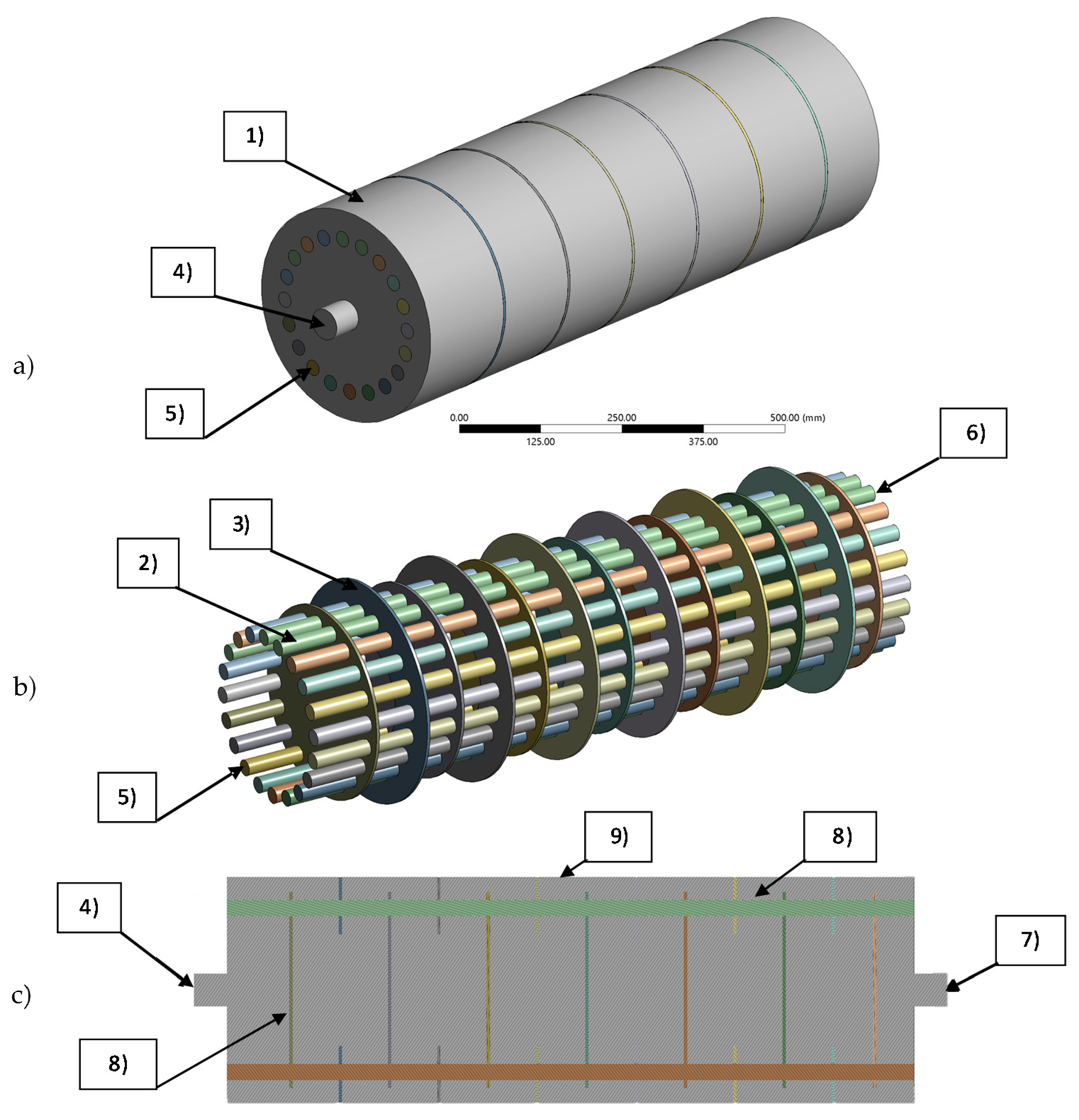
Figure 3.
Model mesh.(a) All domains; (b) Tubes and baffles sub-domains; (c) Tubes inlet detail. (1) Tetrahedral mesh in coolant domain. (2) Inflation layers detail at tubes wall. (3) Hexahedral mesh in tube domains. (4) Hexahedral mesh at Disk type baffle. (5) Hexahedral mesh at Doughnut type baffle. (6) and (7) Non-conformal interface zones, between coolant and tubes/baffles domains.
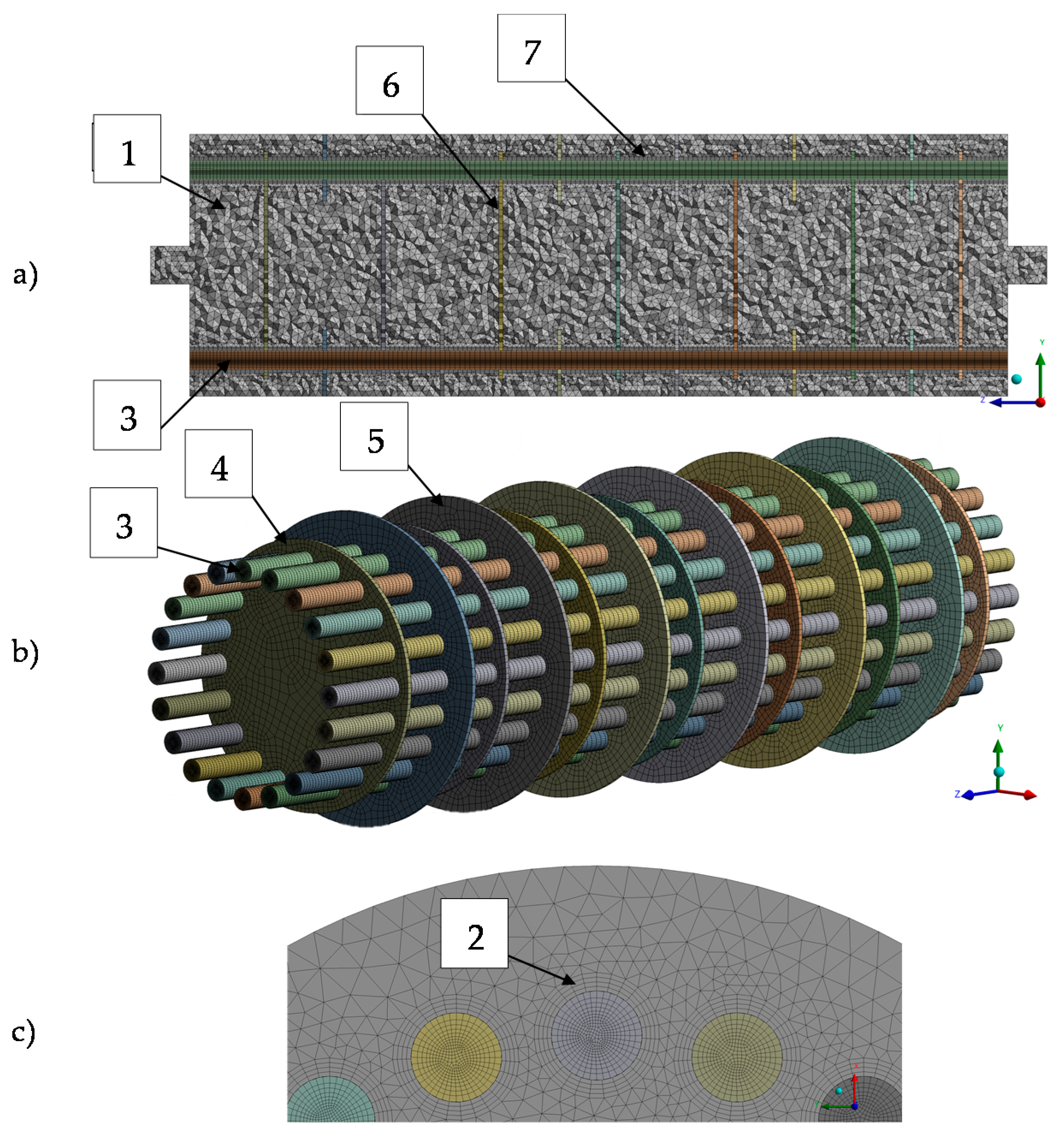
Figure 4.
Transient axial temperature profiles inside reactor tubes for: (a) Start-up and (b) Shutdown operation. Steady state reached after 330 s (a), and reactor Shutdown reached after 130 s of H2 feed interruption (b).
Figure 4.
Transient axial temperature profiles inside reactor tubes for: (a) Start-up and (b) Shutdown operation. Steady state reached after 330 s (a), and reactor Shutdown reached after 130 s of H2 feed interruption (b).
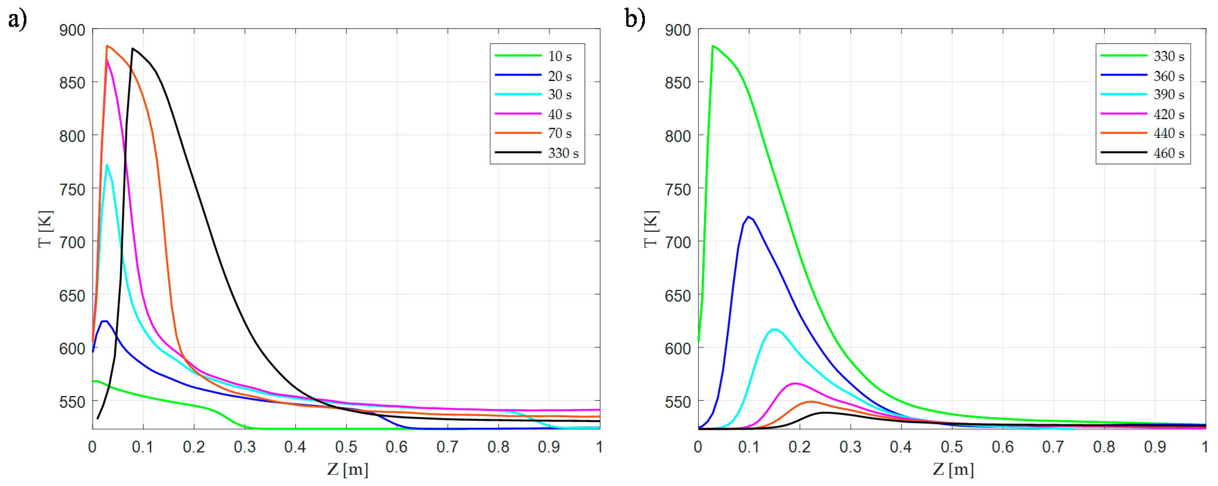
Figure 5.
Temperature contours in the hot-spot relevant zone (First 500 mm of reactor tube length) for: Start-up operation: (a) 10 s, (b) 20 s, (c) 40 s, (d) 330 s and Shut-down operation: (e) 365 s, (f) 405 s, (g) 460 s.
Figure 5.
Temperature contours in the hot-spot relevant zone (First 500 mm of reactor tube length) for: Start-up operation: (a) 10 s, (b) 20 s, (c) 40 s, (d) 330 s and Shut-down operation: (e) 365 s, (f) 405 s, (g) 460 s.
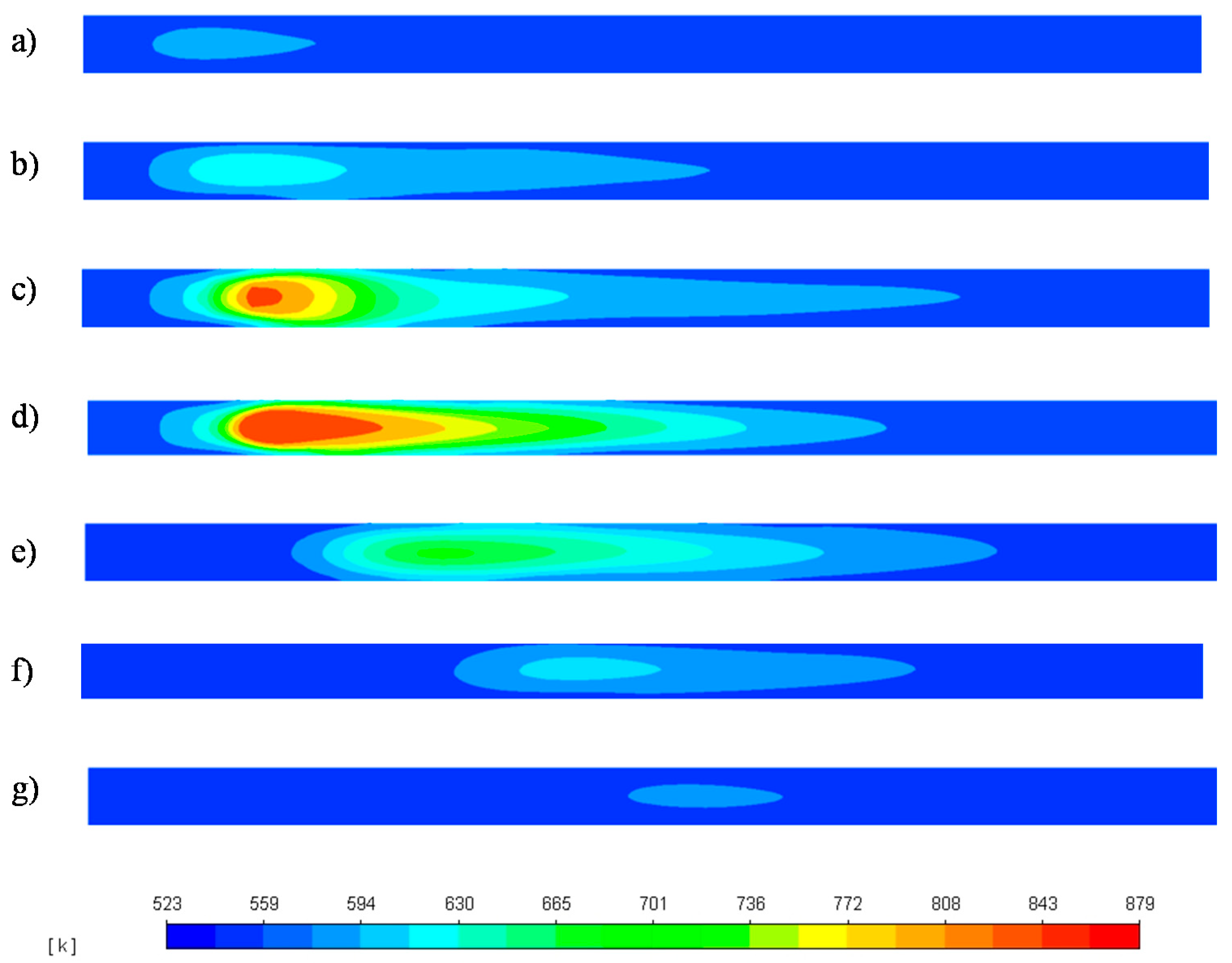
Figure 6.
Temperature contours in the hot-spot relevant zone after a 30 s H2 feed disruption at t: (a) 360 s, (b) 380 s, (c) 400 s, (d) 450 s.
Figure 6.
Temperature contours in the hot-spot relevant zone after a 30 s H2 feed disruption at t: (a) 360 s, (b) 380 s, (c) 400 s, (d) 450 s.

Figure 7.
Effect of a 30 s H2 feed disruption on the methane mole fraction at reactor outlet and the maximum reactor temperature. H2 feed disruption occurs from 330 s to 360 s (from reactor standby). At 360 s, H2 feed is resumed. The original steady state is completely recovered at t = 450 s.
Figure 7.
Effect of a 30 s H2 feed disruption on the methane mole fraction at reactor outlet and the maximum reactor temperature. H2 feed disruption occurs from 330 s to 360 s (from reactor standby). At 360 s, H2 feed is resumed. The original steady state is completely recovered at t = 450 s.
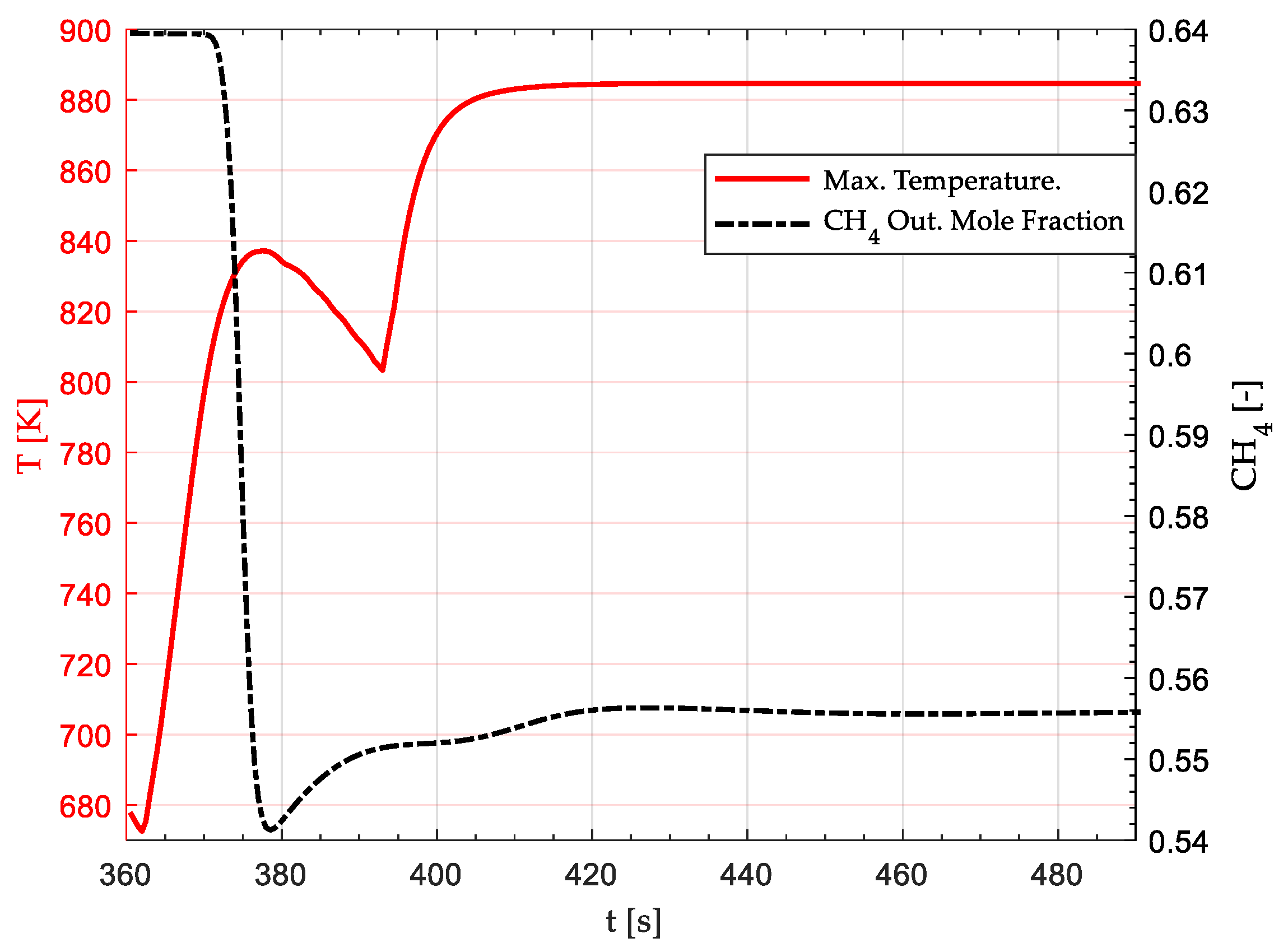
Figure 8.
Temperature contours in the hot-spot relevant zone after a 20 K step-rise in the feed gas (523 K to 543 K) at t = (a) 10 s, (b) 20 s, (c) 30 s, (d) 120 s from disruption.
Figure 8.
Temperature contours in the hot-spot relevant zone after a 20 K step-rise in the feed gas (523 K to 543 K) at t = (a) 10 s, (b) 20 s, (c) 30 s, (d) 120 s from disruption.
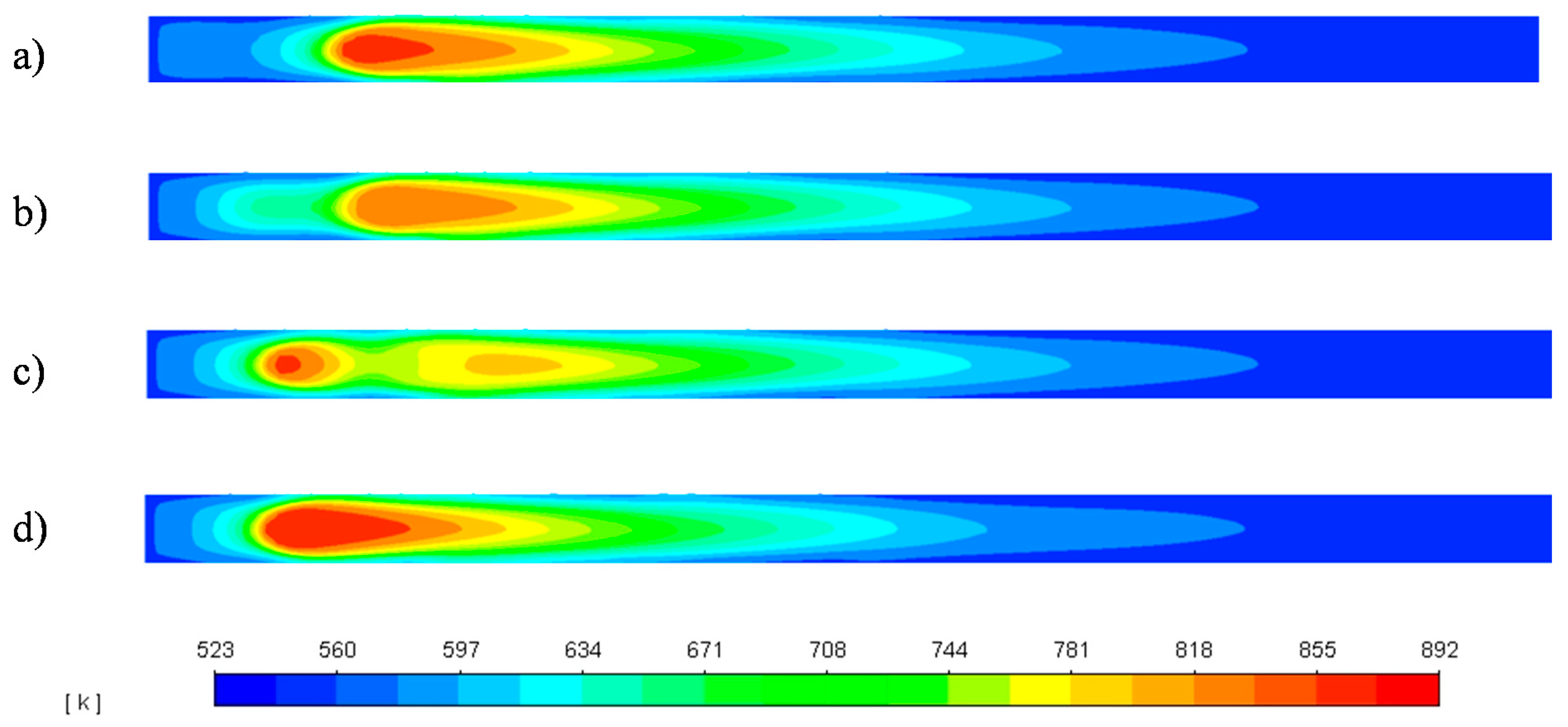
Figure 9.
Effect of a 20 K step-rise in the feed gas (523 K to 543 K) on the maximum (Hot Spot) reactor temperature and CH4 average outlet mole fraction. The disruption begins at t = 0, and a new steady state is established after t ≈ 120 s.
Figure 9.
Effect of a 20 K step-rise in the feed gas (523 K to 543 K) on the maximum (Hot Spot) reactor temperature and CH4 average outlet mole fraction. The disruption begins at t = 0, and a new steady state is established after t ≈ 120 s.
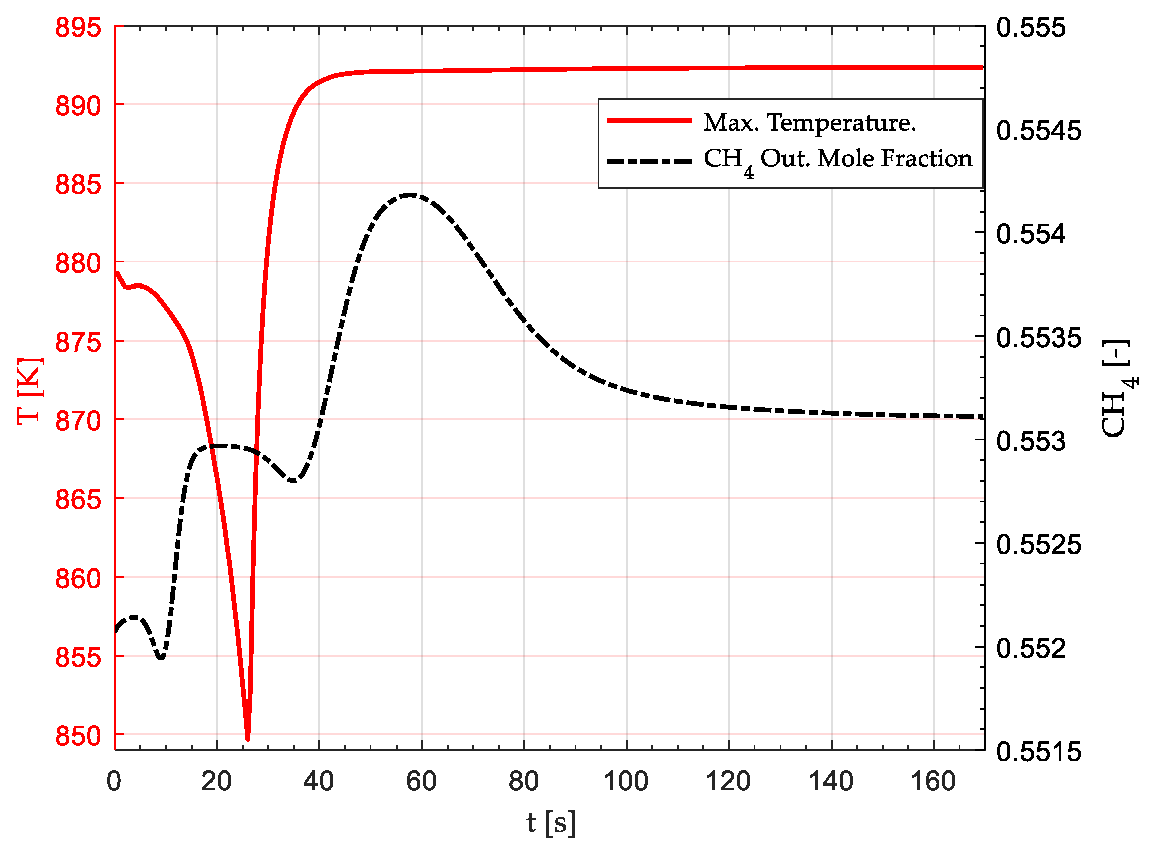
Figure 10.
CO2 mole fraction contours in the hot-spot (First 250 mm of reactor tube length) after a 20 K step-rise in the feed gas (523 K to 543 K) at t = (a) 0 s, (b) 10 s, (c) 30 s from disruption. The concentration front successively moves upwards due to the effect of larger reaction rates near the inlet.
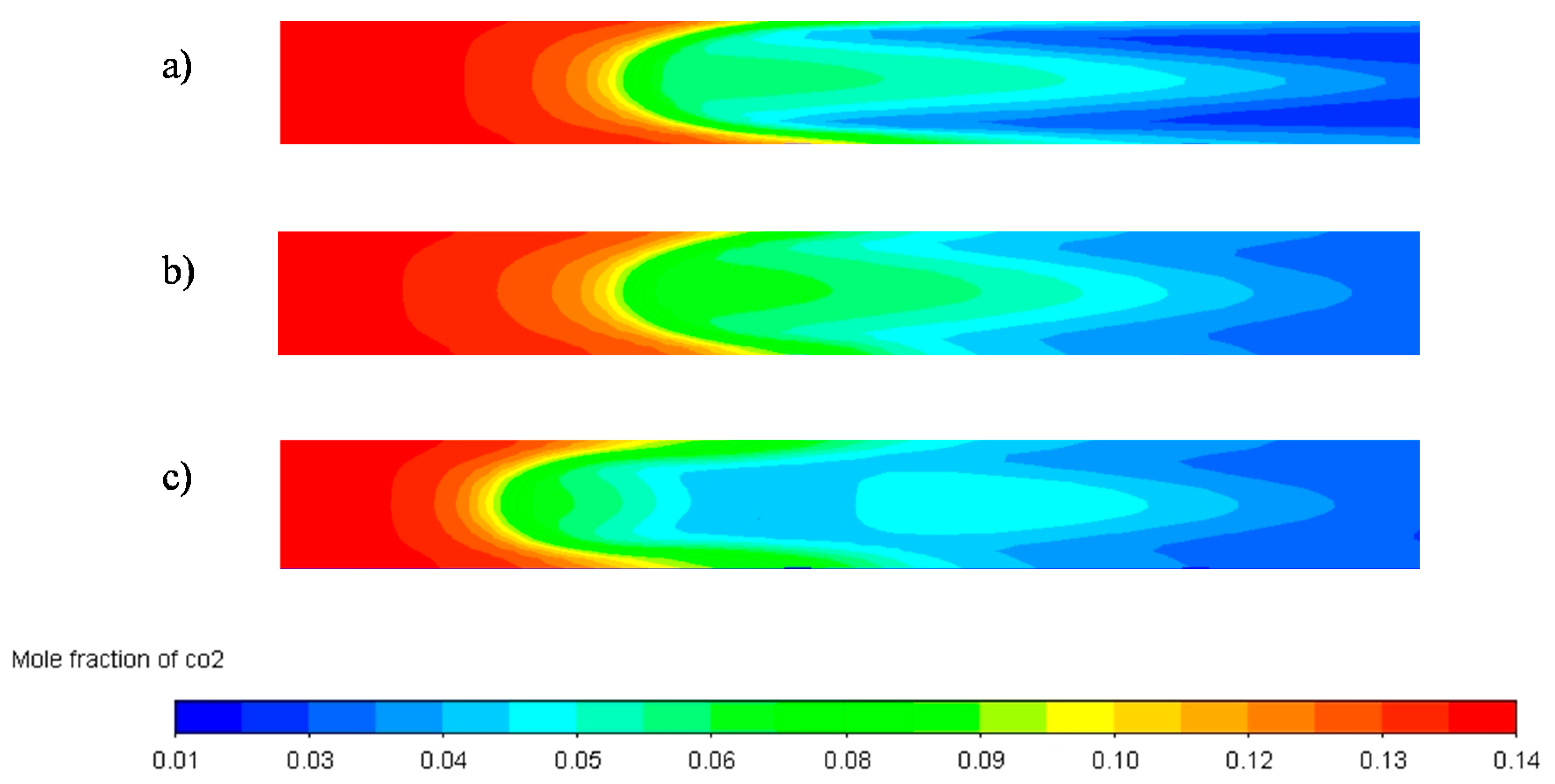
Figure 11.
Effect of 20 K inlet temperature rise on the reactor. Hot-spot position and coolant velocity overlay field at t = 120 s.
Figure 11.
Effect of 20 K inlet temperature rise on the reactor. Hot-spot position and coolant velocity overlay field at t = 120 s.

Figure 12.
Temperature contours in the hot-spot relevant zone after a 20 K step-drop in the feed gas (523 K to 503 K) at t = (a) 10 s, (b) 20 s, (c) 30 s, (d) 60 s, (e) 200 s from the disruption.
Figure 12.
Temperature contours in the hot-spot relevant zone after a 20 K step-drop in the feed gas (523 K to 503 K) at t = (a) 10 s, (b) 20 s, (c) 30 s, (d) 60 s, (e) 200 s from the disruption.
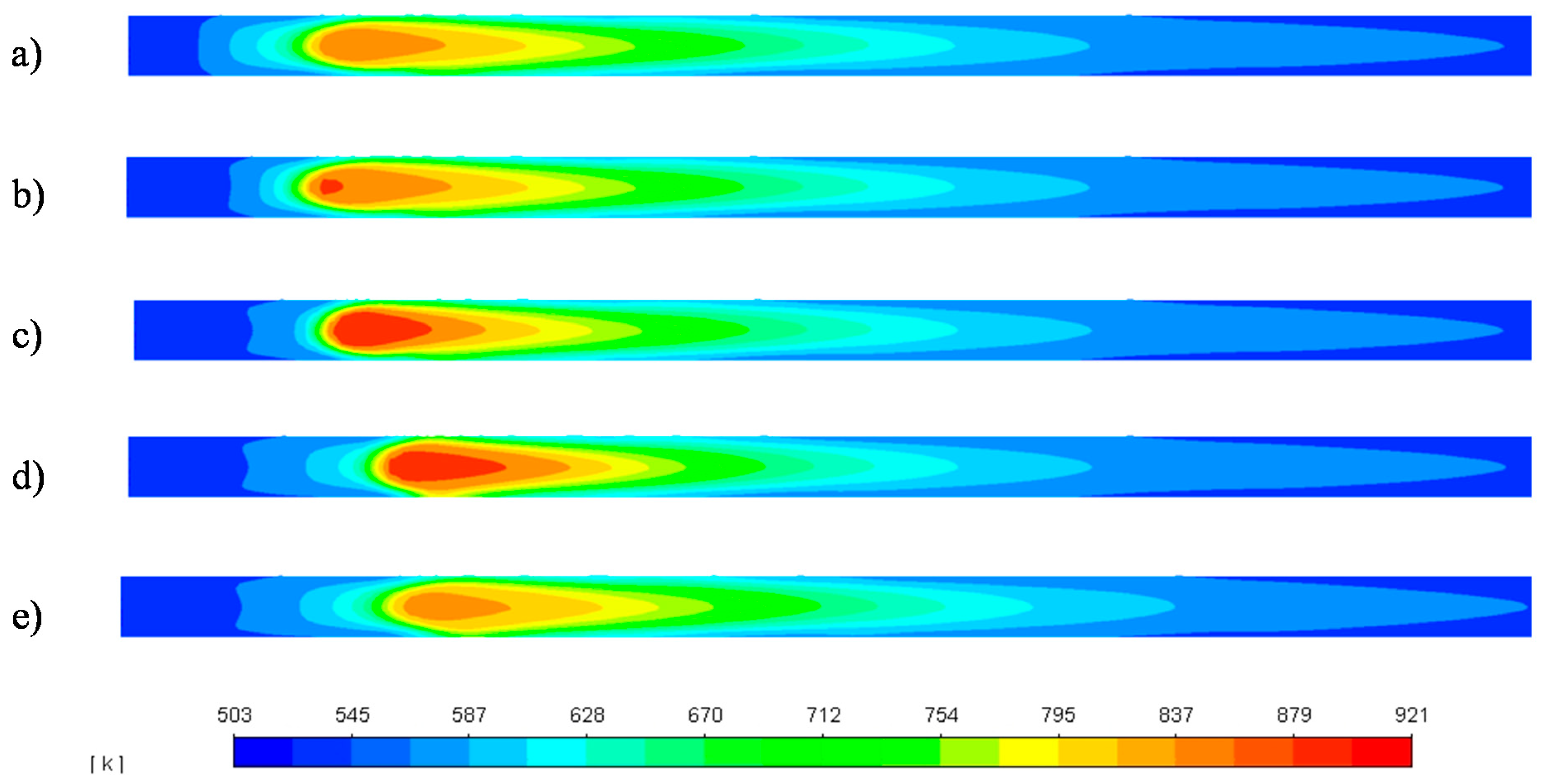
Figure 13.
Effect of a 20 K step-drop in the feed gas (523 K to 503 K) on the maximum (Hot Spot) reactor temperature and CH4 average outlet mole fraction. The disruption begins at t = 0, and a new steady state is established after t ≈ 200 s.
Figure 13.
Effect of a 20 K step-drop in the feed gas (523 K to 503 K) on the maximum (Hot Spot) reactor temperature and CH4 average outlet mole fraction. The disruption begins at t = 0, and a new steady state is established after t ≈ 200 s.
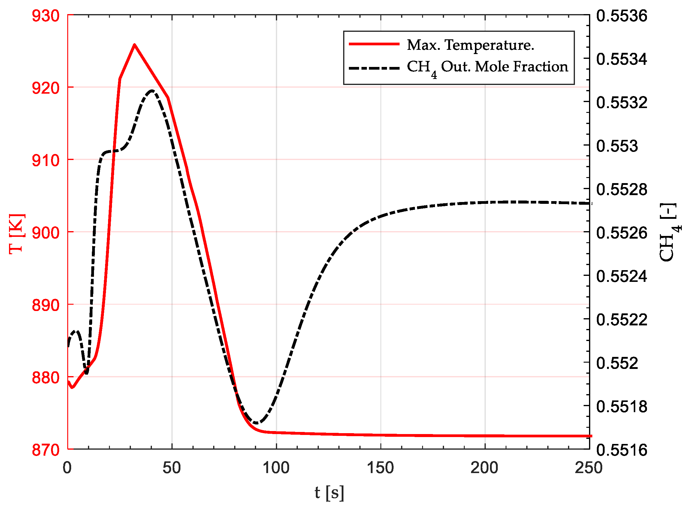
Figure 14.
CO2 mole fraction contours in the hot-spot (First 250 mm of reactor tube length) after a 20 K step-drop in the feed gas (523 K to 503 K) at t = (a) 10 s, (b) 20 s, (c) 40 s from disruption. The concentration front successively moves downwards due to lower reaction rates near the inlet. A maximum concentration gradient is observed in (c), which coincides with the maximum temperature in Figure 12a.

Figure 15.
Effect of 20 K inlet temperature drop on the reactor. Hot-spot position and coolant velocity overlay field at t = 200 s.
Figure 15.
Effect of 20 K inlet temperature drop on the reactor. Hot-spot position and coolant velocity overlay field at t = 200 s.
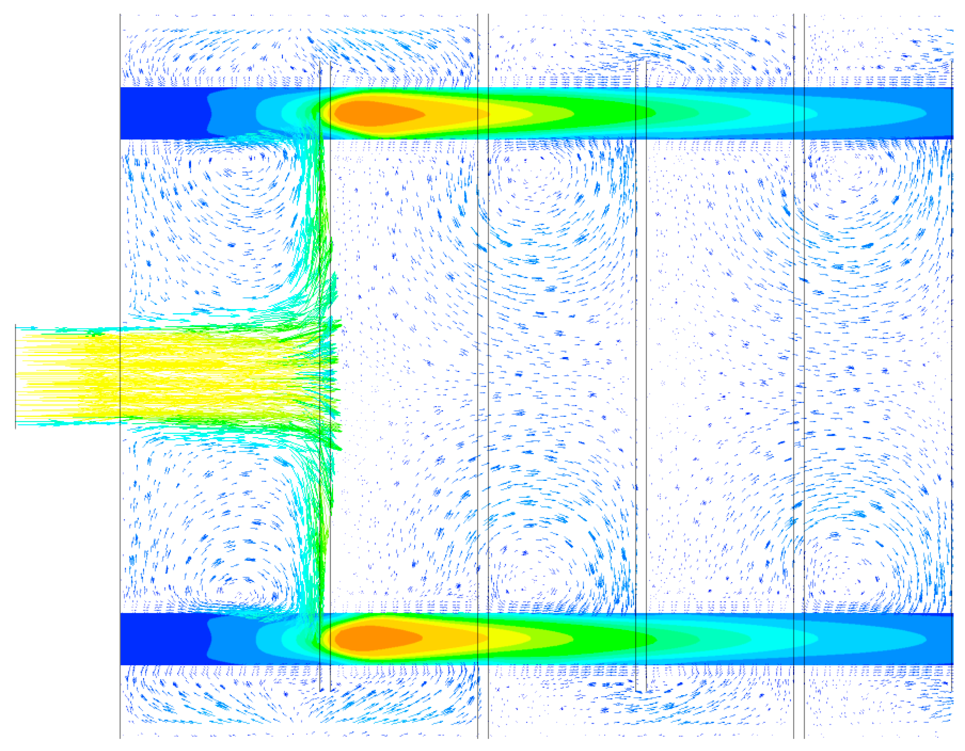
Figure 16.
Reactor YZ plane temperature contours after (a) one, (b) three, and (c) five hours of no coolant/gas flow.
Figure 16.
Reactor YZ plane temperature contours after (a) one, (b) three, and (c) five hours of no coolant/gas flow.

Table 1.
Operational conditions and reactor technical specifications.
| Parameter | Unit | Value |
|---|---|---|
| Reactor dimensions | ||
| Tube outside diameter | mm | 25 |
| Tube length (First module) | mm | 975 |
| Tube length (Second module) | mm | 500 |
| Number of tubes | - | 20 |
| Insulation [17] | ||
| Material | - | Mineral wool |
| Thickness | mm | 50 |
| Density | kg/m3 | 700 |
| Specific Heat | j/kg∙K | 2310 |
| Thermal conductivity | W/m∙K | 0.05 |
| Operational parameters | ||
| Biogas flow | Nm3/h | 20 |
| Reaction pressure | bar | 10 |
| Gas feed temperature | K | 523 |
| Cooling temperature | K | 523 |
| Catalyst maximum temperature [16] | K | 923 |
| Coolant flow | m3/h | 3.5 |
| GHSV | h−1 | 3200 |
| Gas flow per tube | Nm3/h | 1.5 |
| Feed gas composition | ||
| CH4 inlet mole fraction | mol/mol | 0.280 |
| CO2 inlet mole fraction | mol/mol | 0.146 |
| H2 inlet mole fraction | mol/mol | 0.550 |
| H2O inlet mole fraction | mol/mol | 0.015 |
| O2 inlet mole fraction | mol/mol | 0.004 |
Table 2.
Comparison of industrial sized biogas methanation reactors.
| Reactor Type | Reactor Tubes Dimensions [DxL] | Biogas/Total Flow [Nm3/h] | Inlet Temperature [K] | Pressure [bar] | XCO2 [%] | Cooling System | Study Type | Comments | Reference |
|---|---|---|---|---|---|---|---|---|---|
| Two stage multi tube packed bed | 25 mm × 1 m 25 mm × 0.5 m | 20 | 523 | 10 | 91 ≈99 | Shell side thermal oil 523 K | Numerical CFD | 20 tubes | This work |
| Multi tube packed bed | 45 mm × 4 m | 100 | 473–573 | 8–40 | 94–98 | Shell side thermal oil 519 K | Numerical | 60 tubes | [18] |
| Multi tube packed bed | 20 mm × 8 m | 450 | 476 | 1 | 96 | Shell side Boiling Water | Numerical | 1950 tubes | [19] |
| Single tube packed bed | 200 mm × 1 m | - 382.5 | 550 | 5 | ≈80 | Shell-side Molten Salt tubes 600 K | Numerical | 13 cooling tubes | [20] |
| Three step multi tube packed bed with interstage condensation | 10 mm × 1.13 m 10 mm × 0.95 m 10 mm × 0.36 m | 1612 | 526 515 513 | 13.6–13.9 | 62 91 99.5 | Shell side Molten Salt | Optimisation | 588 tubes | [21] |
| Multi tube packed bed | 9.25 mm × 250 mm | 100 | 473 | 5 | 99 | Tube wall set at T = 373 K | Numerical CFD | 1000 tubes | [22] |
| Two stage multi tube packed bed | 25 mm × 3.5 m 25 mm × 5 m | 200 | 613–673 | 7–45 | >90 | Shell side cooled | Process design | N/A | [23] |
| Multi tube packed bed | Same as [21] | Same as [21] | 442–526 | 13.4–13.9 | Same as [21] | Shell side cooled 500–515 | Exergetic analysis | Same as [21] | [24] |
| Two stage multi tube packed bed | 2.3 m length | 10 | 553.15 | 20 | ≈100 | Boiling water 280 °C-65 bar | Experimental | 2 tubes in series | [2] |
| Four stage multi tube packed bed | 50 mm × 4 m | 8–16 | 473.15 | 15 | 90 | Thermal oil 370 °C | Experimental | 4 tubes in series | [3] |
| Two stage multi tube packed bed | 25.4 mm × 3 m | 0.4–0.64 | 500–600 | 1–15 | 90–99 | - | Numerical thermodynamic | 20–24–28 | [25] |
Table 3.
Governing equations of the transient CFD model.
| Reactive Flow (Tubes) |
|---|
| Gas phase continuity: |
| Gas phase momentum: |
| Gas phase Energy: |
| Species: |
| Coolant flow (shell-side): |
| Fluid phase continuity: |
| Fluid phase momentum: |
| Fluid phase energy: |
| Baffles & tube walls: |
| Solid phase energy: |
Table 4.
Boundary and cell zone conditions.
| Condition | Unit | Value | Cell Zone |
|---|---|---|---|
| Velocity inlet | m/s | 0.5 | Coolant |
| Pressure (static) outlet | Pa | 0 | Coolant |
| Convective heat transfer coefficient | W·m2·K−1 | 5 | Coolant |
| Free stream temperature | K | 300 | Coolant |
| Thermal coupled wall | - | - | Interface Coolant/Tubes |
| Mass flow inlet | kg/s | 2.15 × 10⁻⁴ | Tubes |
| Pressure outlet | Pa | 0 | Tubes |
| Operating pressure (coolant) | Pa | 1.013 × 10⁵ | Coolant |
| Operating pressure (tubes) | Pa | 1.013 × 10⁶ | Tubes |
| Symmetry (tubes inlet/outlet) | - | - | Tubes (stand by simulation) |
| Symmetry (coolant inlet/outlet) | - | - | Coolant (stand by simulation) |
Table 5.
Mesh details.
| Sub-Domain | Nodes | Elements | Average Skewness | Average Aspect Ratio | Average Orthogonal Quality |
|---|---|---|---|---|---|
| Fluid | 750,818 | 2,406,886 | 0.34141 | 3.0043 | 0.65751 |
| Tubes (×20) | 1,262,360 | 1,191,000 | 0.11051 | 8.3040 | 0.98924 |
| Doughnut Baffles (×6) | 21,564 | 9150 | 0.18852 | 1.5399 | 0.96949 |
| Disk Baffles (×6) | 21,168 | 9054 | 0.18358 | 1.5027 | 0.97285 |
| Total | 2,055,910 | 3,616,090 | 0.27069 | 4.4693 | 0.76151 |
Publisher’s Note: MDPI stays neutral with regard to jurisdictional claims in published maps and institutional affiliations. |
© 2022 by the authors. Licensee MDPI, Basel, Switzerland. This article is an open access article distributed under the terms and conditions of the Creative Commons Attribution (CC BY) license (https://creativecommons.org/licenses/by/4.0/).
Share and Cite
MDPI and ACS Style
Soto, V.; Ulloa, C.; Garcia, X. A 3D Transient CFD Simulation of a Multi-Tubular Reactor for Power to Gas Applications. Energies 2022, 15, 3383. https://doi.org/10.3390/en15093383
AMA Style
Soto V, Ulloa C, Garcia X. A 3D Transient CFD Simulation of a Multi-Tubular Reactor for Power to Gas Applications. Energies. 2022; 15(9):3383. https://doi.org/10.3390/en15093383
Chicago/Turabian StyleSoto, Victor, Claudia Ulloa, and Ximena Garcia. 2022. "A 3D Transient CFD Simulation of a Multi-Tubular Reactor for Power to Gas Applications" Energies 15, no. 9: 3383. https://doi.org/10.3390/en15093383
Note that from the first issue of 2016, this journal uses article numbers instead of page numbers. See further details here.