
A Straightforward Approach to Site-Wide Assessment of Wind Turbine Tower Lifetime Extension Potential


1
Wind & Marine Centre for Doctoral Training, University of Strathclyde, Glasgow G1 1XQ, UK
2
Wind Energy & Control Centre, EEE, Faculty of Engineering, University of Strathclyde, Glasgow G1 1XW, UK
*
Author to whom correspondence should be addressed.
†
These authors contributed equally to this work.
Energies 2022, 15(9), 3380; https://doi.org/10.3390/en15093380
Submission received: 25 March 2022
/
Revised: 22 April 2022
/
Accepted: 28 April 2022
/
Published: 6 May 2022
(This article belongs to the Special Issue Lifetime Extension of Wind Turbines and Wind Farms)
Abstract
:This contribution presents a novel methodology to evaluate the lifetime extension potential of wind turbines—taking towers as the key component that preserves onshore turbines’ structural integrity—as a consequence of the difference between design and site-specific loads. Specifically, attention is drawn to the site-specific wind direction distribution, which provides an additional source of lifetime extension potential. For this purpose, variants of closed-form solutions (based on the tower section’s normal stress) are developed to enable fatigue damage accumulation due to fore-aft and side-to-side bending moments at any point on the tower circumference without the need for further information on tower section geometry or material properties. Based on the degree of data availability, different scenarios are defined to estimate lifetime extension potential from the accurate tower’s normal stress and approximations using resultant bending moment, fore-aft bending moment, and finally, wind rose data only. The methodology is applied to a wind farm case study using the actual SCADA data with a partially validated turbine’s aeroelastic model to obtain operational loads. The results indicate that this quick and fairly accurate approach can be used as an initial stage in identifying wind turbines across large farms, which have the largest lifetime extension potential.
1. Introduction
As the wind energy assets are beginning to age and reach the end of their design life across Europe, there are three options available to owners and operators, namely, decommissioning, repowering and lifetime extension. Decommissioning is the default approach once the design life is reached [1]. All components are removed, and this option provides no additional benefits [1]. Repowering allows for modification or replacement of components, such as larger blades, in order to increase the power rating and extend the life of the turbine, but can have cost, environmental and legal constraints [1,2]. The third option is lifetime extension, which investigates whether there is potential for the existing wind turbine components to operate longer than their design life and is the focus of this study.
The process of carrying out lifetime extension is complex since economical, technical and legal aspects all need to be considered [1]. The legal aspects are not covered here. The economical aspect appears to focus on cost-benefit analysis. If the cost-benefit analysis proves that revenue generated from lifetime extension is greater than the expense of the additional inspection, operation and maintenance associated with extending the life of the turbine, then the wind turbine’s operating life is extended beyond the design lifetime. Since an evaluation of lifetime potential is carried out towards the end of the lifetime of the wind turbine/farm, the additional costs for replacement or modification tend to be less than that for repowering, and lifetime extension can allow for greater profit [1,3]. The economical aspects of lifetime extension will not be discussed further within this study, and this work focuses on the technical aspects in terms of lifetime extension potential assessment.
For the sake of the technical assessment, several guides to lifetime extension exist, for instance, those developed by DNV GL [4], Bureau Veritas [5] and Megavind [6]. Additionally, other companies such as Siemans Gamesa [7] and Nabla Wind Power [8] have started to offer a lifetime extension service for their own turbines. Although there is an active task introduced by IEC TC-88/PT 61400-28 in order to publish the so-called “Through life management and life extension of wind power assets’ [9], at present, there is no agreed standardised process or application for lifetime extension. Therefore, it is timely for researchers in the area of lifetime extension to raise technical and practical awareness for the sake of standardisation. In general, within the process for lifetime extension in terms of the technical aspects, the focus appears to include fatigue load assessment on the wind turbines components, identifying the remaining useful life based on the total site-specific fatigue damage and its comparison to the design life [10], while taking the safety and economic aspects into account. The wind turbines’ components, such as the foundation and tower, are expected to be the main components considered for wind turbine lifetime extension when it comes to primarily preserving the structural integrity of the turbine. In terms of continuation of the operation beyond the design life, the lifetime extension potential of electro-mechanical components such as those within the drivetrain has to be also evaluated [11], which is outside the scope of this contribution.
According to the standard IEC 61400-1 [12], wind turbine design is based on turbine classes, which are dependent on the mean wind speed and turbulence intensity. The wind turbine components are required to withstand the design load cases (DLC) for a lifetime of at least 20 years, i.e., the normal design life. The frequency of occurrence of each load condition, in which the turbines are expected to operate for the majority of their life span, is determined by the mean wind speed distribution. As such, the turbine components’ design should provide the capacity to withstand the loading cycles for that mean wind speed distribution, excluding wind direction variability effects. The wind direction variability is not very influential on the nacelle-rotor assembly components due to the yaw mechanism, whereas it results in a conservative tower design based on a worst-case scenario assumption. These design loads are considered when looking at lifetime extension—in particular, the cyclic fatigue loads.
There are different approaches to establishing fatigue loads and assessing lifetime extension potential. Such methods can employ numerical wind turbine simulation models [4,5], take into account current environmental and operating conditions using SCADA [10] or direct measurement and structural health/condition monitoring [5,13,14]. Other methods based on inspection only or inspection in conjunction with simulation or measured data have also been suggested by Ziegler et al. [10].
Rubert et al. [13] and Kazemi Amiri et al. [15] both investigated lifetime extension for onshore wind turbine towers. Rubert et al. [13] used a symmetrical tower, whereas Kazemi Amiri et al. [15] considered the door opening impact on the tower stresses through a detailed finite element modelling and analysis.
Rubert et al. [13] used a structural health monitoring approach taking data from optical strain gauges located on a 2 MW wind turbine tower. The four strain gauge positions were intended to be located parallel and perpendicular to the prevailing wind direction identified using SCADA data. Converting the strain data into stresses and identifying the largest occurrence of stress at the fore-aft natural frequency, the largest fatigue damage and, therefore, critical points on the tower were identified by Rubert et al. [13].
A novel approach by Natarajan and Pedersen [16] considered the use of curtailment to provide an extension to tower life. Natarajan and Pedersen curtailed the wind turbine power output when high levels of turbulence were detected. Taking this approach, which was based on modifying the turbine operation regime, they showed the tower fatigue load was reduced, and accordingly, there is the potential for the turbine’s life extension [16].
Slot et al. [17] investigated whether assuming the worst-case scenario—a uni-directional wind—was the best approach. Proposing approximation models to represent the fatigue loads due to wind directionality, their resulting fatigue loads, taking into account directionality, were then compared to maximum fatigue damage representing the uni-directional or maximum fatigue damage. Although Slot et al. [17] did not consider lifetime extension, their approximate results on tower fatigue load estimation indicated that assuming uni-directional turbulent wind —a uni-directional wind— as outlined in the standards —a uni-directional wind— led to average overestimations of tower fatigue damage. As such, this conservative approach to the design standard, which could evidently demonstrate the potential for lifetime extension under site-specific loads, is worth further investigation.
Since there is still no standard methodology to assess lifetime potential for onshore wind turbines to date, there are open questions on the methods and implementation as well as the sources of lifetime extension potential. Wind turbine lifetime extension is indeed a complex task comprising different analyses and control procedures to assess the condition of various structural, mechanical and electrical components, followed by their regular inspection programme. Primary components in terms of life time extension, such as tower, foundation, blades pitch and yaw bearings, are located along the turbine’s load path to preserve the structural integrity of the system. These primary components are usually very difficult to replace or very costly to repair, whereas the secondary components normally require maintenance and undergo regular repairs over the turbine’s lifetime. In this paper, a straightforward approach to lifetime extension potential assessment is presented, when bending moment or bending stress time series and wind speed data are available. The focus is on the tower as one of the main elements of the turbine’s structural integrity. This work studies the life extension potential of the turbine tower for the combination of different scenarios and situations that are defined based on the data availability and the required level of accuracy in practical applications. A simple approach using just wind rose data is also presented as a rough measure of damage distribution with respect to the wind directions.
The structure of this paper is as follows: Section 2 discusses the methodology for lifetime extension potential. To this end, different approximation methods in combination with a range of possible scenarios based on the varied level of available data are introduced. Section 3 investigates the application of the proposed methodology and inspects the fatigue damage results for a single turbine. The implementation of the methodology on a wind farm case study is presented in Section 4 to illustrate the procedure for estimating the lifetime extension potential and its variations across the farm. Finally, the conclusion and remarks are summarised in Section 5.
2. Damage Estimation for Turbine Towers
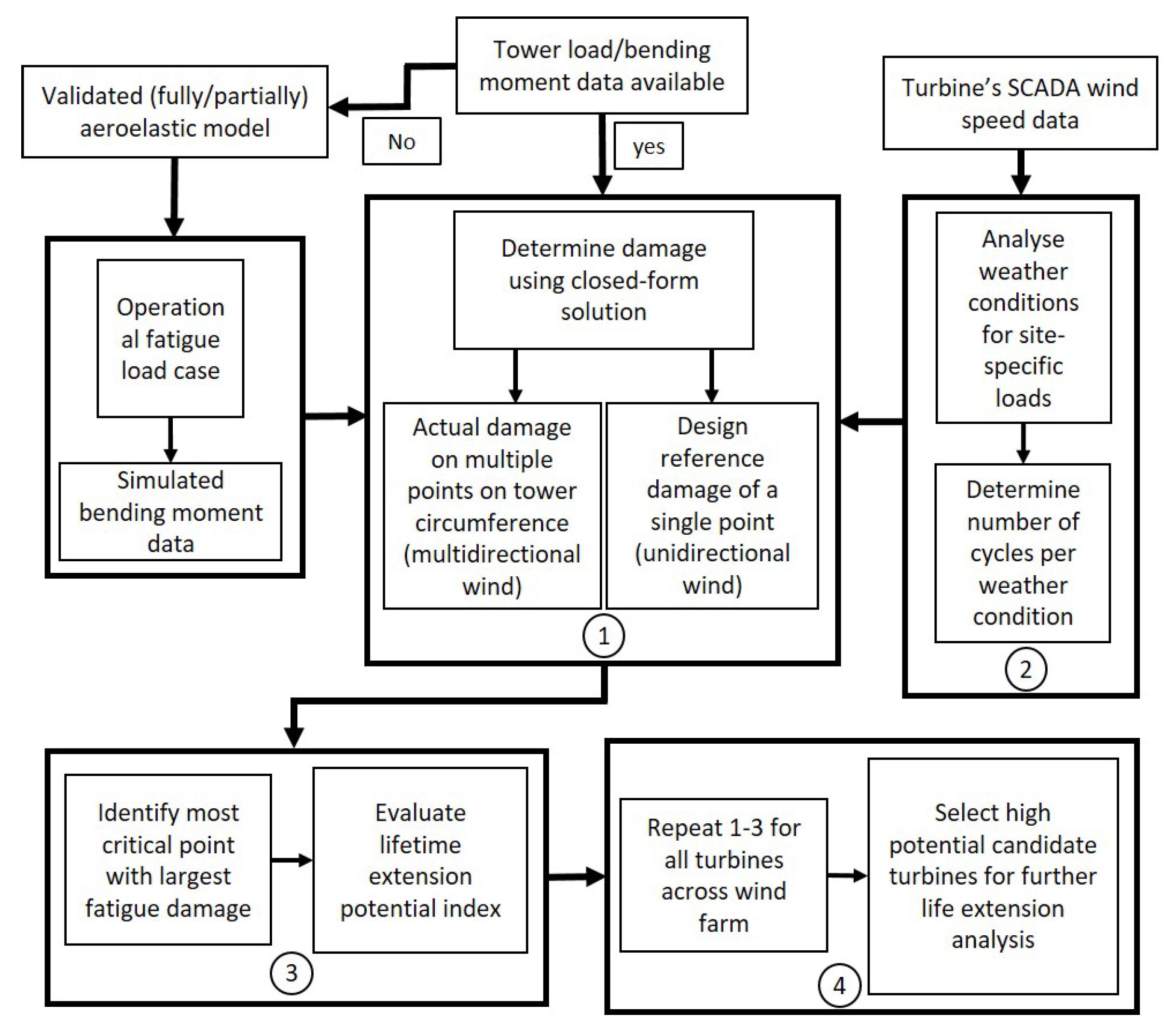
A lifetime extension assessment is going to be carried out for large onshore wind farms comprising tens of wind turbines; the aim of this contribution is to develop a methodology through which those individual wind turbines with high potential for lifetime extension within the large farms can be shortlisted. Here, the presumed criterion that determines this potential is an evaluation of the residual tower’s life capacity relative to a representative turbine on the same farm, as the tower is considered as the key element of the wind turbine’s structural integrity. On the basis of this idea, this work proposes a methodology to evaluate the lifetime extension potential of wind turbine towers, which is summarised in Figure 1. The output of this proposed procedure is those candidate turbines with the highest potential for lifetime extension. Subsequently, these candidate wind turbines should be further analysed for a detailed lifetime extension assessment, a step which falls outside the scope of this paper. The flowchart of the procedure for lifetime extension potential assessment is presented in Figure 1.
The procedure provided in Figure 1, retains some of the fundamental elements of the methodology by Kazemi Amiri et al. in [15], where the fatigue damage is calculated using stress results at concentration points around the door opening and tower base through finite element analysis (FEA). However, if the tower is positioned properly relative to the prevailing wind directions such that the critical damage point will not fall in the door surrounding areas, then the door opening effect can be omitted. In this situation, the methodology in Figure 1 is modified here to include a closed-form solution for fatigue damage estimation at any tower cross section from turbine load data. This makes the current methodology more practical as a straightforward tool for an initial assessment of lifetime extension potential. According to the flowchart in Figure 1, the basic assumption is that tower bending moment data at any section along the tower are inputted into the procedure (on the left of box 1). The load data are either available from direct measurement or can be obtained via the turbine’s load simulation, e.g., by an aeroelastic analysis. Furthermore, the wind speed data can be accessed, e.g., from the turbine’s SCADA (box 2).
For the evaluation of lifetime extension, it is key to compare the operational (site-specific) loads with those of the reference design. The procedure within box 1 basically feeds box 3 with the results for this assessment to be carried out. To this end, the tower design reference damage is considered to comply with the IEC 61400-1 standard [12], based on the turbine class for certain reference mean wind speed and turbulence intensity. While the design standard conservatively assumes a uni-directional wind with a specific mean wind speed probability distribution, the operational turbine loads are caused by multi-directional wind conditions. Taking this point into account, the lifetime extension potential for the tower can then stem from two sources; firstly, milder site conditions than in the standards and secondly, the lower damage incurred at a single point on the tower circumference due to the standard’s presumed uni-directional wind compared with the actual uni-directional wind. Note that among these two sources, only the former is taken into account by most of the existing guidelines for life extension, whereas the latter provides additional potential, particularly for towers and foundations. The variability of wind direction and the random distribution of the mean wind speed across different directions results in a specific point on a given tower cross section, which undergoes the highest fatigue damage and is unknown a priori. Therefore, this point needs to be identified (first of box 3) as a critical stress location that determines the tower life. This requires the fatigue damage to be evaluated on several points around the tower cross section, which can be readily performed using the developed closed-form solutions later within this section.
Within this procedure, it is assumed that no further information on tower section geometrical or material properties are available, or if it is available, the information does not enable the remaining useful life to be definitely estimated through fatigue damage analysis due to its uncertainty. It is later demonstrated in the subsequent section how this lack of information can be circumvented by definition of an index in terms of the ratio between the uni-directional and multi-directional fatigue damage. This damage ratio is then utilised to evaluate the lifetime extension potential in the second part of box 3.
Finally, it is noted that within box 4 of the methodology flowchart, the lifetime extension potential is evaluated relative to a representative turbine within the same farm. Through this approach, a farm-wide view of the variation of the remaining useful life of all turbines can readily be established. Moreover, the uncertainties associated with the required information for turbine load simulation and/or fatigue damage estimation can be mitigated.
2.1. Closed Form Analytical Solution
Total fatigue damage for any point on the tower circumference, designated by an angle , can be determined as follows:
where represents the joint probability density of mean wind speeds, v, and mean wind directions, , and is the fatigue damage for a specific mean wind speed and wind direction. If required, other wind speed characteristics such as turbulence intensity, wind shear, etc., can also be taken into account in the damage calculation, which requires expanding this integral to consider those variables. However, the standard only takes account of mean wind speed distribution [12].
2.2. Derivation and Application of Closed Form Solution
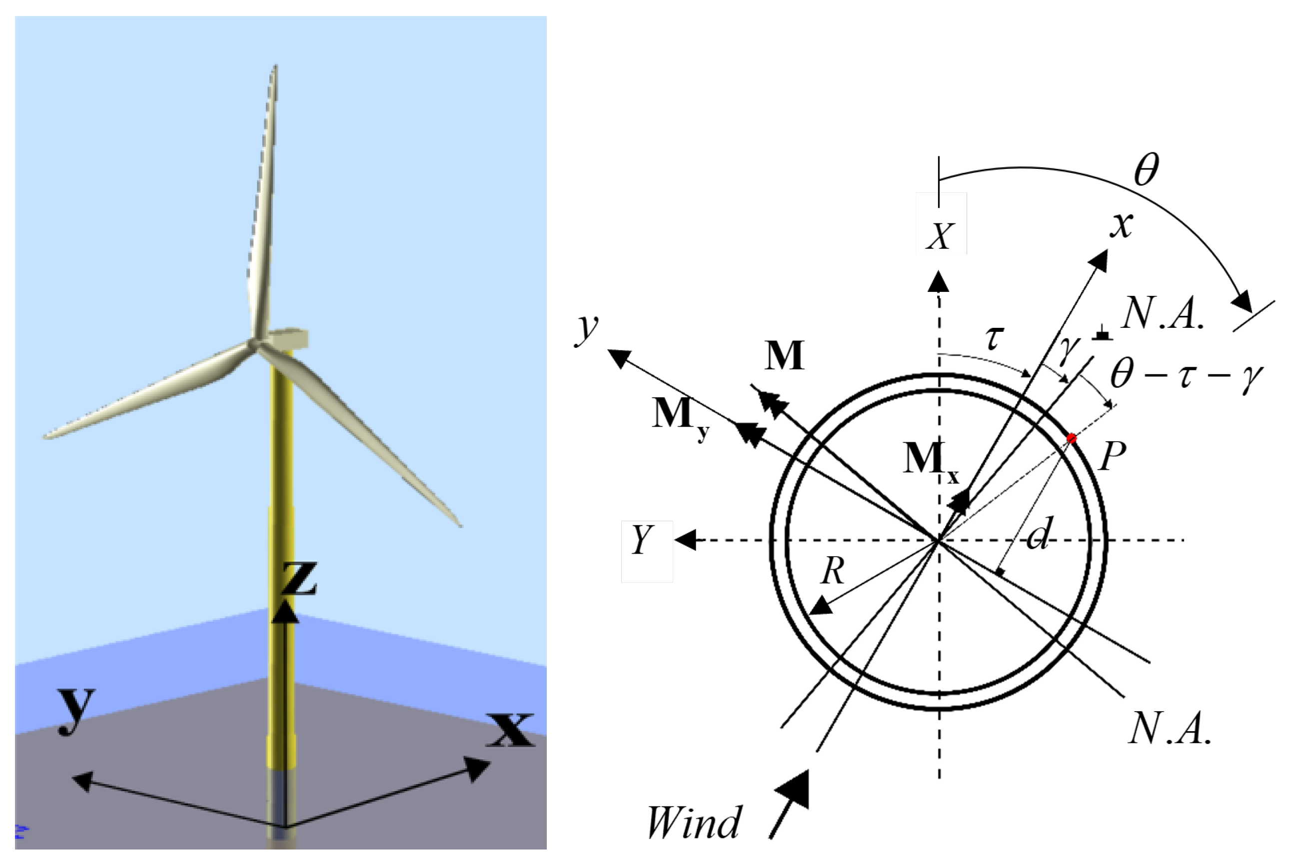
With reference to Equation (1), the derivation of requires determination of the tower’s bending stress. In order to estimate the cumulative damage, integration over all mean wind directions and mean wind speeds is necessary. The co-ordinate system associated with tower’s cross section for this derivation is shown in Figure 2.
2.2.1. Fatigue Damage Derivation
According to the Euler–Bernoulli beam theory, which also applies to design requirements, and accordingly, the analysis of wind turbine towers, bending moment, M, and bending stress, , are related to the tower’s radius of curvature, , as follows:
where y is the distance from the neutral axis to any point on the tower’s cross section, I is the second moment of area and E denotes Young’s Modulus.
As is common practice, the wind turbine tower bending moment can be resolved into a perpendicular (fore-aft) moment, , and a parallel (side-to-side) moment, , relative to the mean wind speed direction. If the normal stress due to axial loads are neglected, the preceding equation can be re-written to express the normal stress, , on an arbitrary point, P, on the tower’s circumference that is located away from north aligned with X direction (see Figure 2):
in which and are the distance of point, P, from the x and y axes, respectively. In the previous equation, the resultant bending moment, M, which resides on the neutral axis of the tower, is:
As in Equation (4), the resultant bending moment is time-dependent and acts on the tower section in given wind conditions and as such is independent of and .
In practice [19], the tower bending moment is obtained through strain measurement at least in two perpendicular directions at two points on the tower cross section. The fore-aft and side-to-side bending moments are resolved by the relative angular position of the measurement axis and wind direction. Since both and vary with time, the phase angle, , namely the angle between the reference north axis and the neutral axis, , and consequently the distance of point, P, from varies continuously:
Substituting Equations (4)–(6) into Equation (3) and considering the so-called sectional modulus, , it renders:
For simplicity, the time dependence of the bending stress on time, t, is not explicitly indicated.
Now, assuming the joint distribution of wind speed and direction for a particular turbine is derived from the turbine’s wind rose, the available information regarding both wind speed and direction would be in discrete form. Consequently, when determining the total fatigue damage, , on the wind turbine tower, the integrals in Equation (1) are replaced by summations over wind speed and direction as shown in Equation (8) and defined using damage equivalent loads, as seen in the final function of Equation (8).
where and are the number and level/amplitude of the stress cycles induced by , and and m are the tower’s steel fatigue and Wohler coefficient.
The bending moment for time t for a given mean wind speed , and given direction, is calculated using , where is the bending moment taken from bending moment data. The term is the equivalent number of cycles to failure used to calculate fatigue damage.
Later on, the underlying assumption is that, for each mean wind speed and direction, the wind speed time series is described by a probability distribution that does not depend on direction. Consequently, the same set of sample wind speed time series can be used for each mean wind speed when calculating bending moments for a particular mean wind speed and direction. Hence, . On the other hand, if the wind speed time series did depend on direction, e.g., the turbulence depended on direction, then turbulence dependent sets of sample wind speed time series would be required. The probability distribution in Equation (8) would then depend on turbulence as well as mean wind speed and direction, and the double summation in Equation (8) would be replaced by a triple summation. Since the wind rose is the only source of directional information, the foregoing assumption has to be made. This leads to Equation (9).
Furthermore, suppose that the wind joint probability distribution is separable, that is, , then:
Therefore, there are four sets of estimates for damage of varying degrees of accuracy:
- (i)
- not assumed to be negligible with Equation (9), where the number and level/amplitude of the stress cycles and are those induced by
- (ii)
- assumed to be negligible with Equation (11), where the number and level/amplitude of the stress cycles are induced by
- (iii)
- assumed to be negligible and Equation (11), where the number and level/amplitude of the stress cycles are induced by the fore-aft bending moment only,
- (iv)
- assumed to be negligible with Equation (12), where the number and level/amplitude of the stress cycles are induced by some generic bending moment
Within the context of wind turbines, as the wind direction varies, any point on the tower will experience both tensile and compressive stresses depending on the alignment with respect to wind direction. Furthermore, as the wind field can be characterised by a mean wind value plus the turbulent fluctuating terms, the turbine structural components will experience stresses with non-zero mean values. To take account of the mean stress effect, some stress amplitude correction methods can be adopted such as application of the Goodman’s correction factor (Equation (13)) to the stress time series (or equivalently load depending on any of the above approximate solutions):
in which , and are the cycle stress amplitude, the mean stress and the ultimate tensile stress, respectively [20]. Whether the tower position, P, is under tensile or compressive loading can simply be determined by evaluation of the value of angle . Position, P, undergoes tensile stress, if the mentioned angle is between 90 and 270 measured clockwise, as shown on the right-hand-side of Figure 2.
Finally, depending on the availability of the turbine load and wind data, different scenarios can be considered for the fatigue damage estimation. In this regard, three scenarios have been subsequently defined.
- Scenario1 —This scenario investigates the lifetime extension potential using either simulated or measured wind turbine load data. The load data are available across varied wind speeds in which the turbine operates and corresponds to a single wind turbine similar to those under investigation and in the same environment (weather conditions). Within this scenario, the wind rose data corresponding to each individual turbine is assumed to be available, e.g., from turbines’ SCADA, which is feasible in practice. In an ideal situation, another scenario can be defined in which the full turbine load and wind data are available for each individual turbine. However, in practice this is not feasible to have the load data of all turbines; thus, the analysis is carried out for a representative turbine.
- Scenario 2 —Where neither simulated nor measured bending moment load data are available, this scenario investigates a rough estimate of lifetime extension potential, as a consequence of wind direction variability, using the wind rose data only, as described in Section 3.3.
Based on these scenarios and their combination with the above approximations (i)–(iv), different sets of damage can be estimated. In this contribution, the proposed methodology uses different sets of estimated damage results that are firstly evaluated for a single case study turbine (Section 3) and then the resulting impacts on the lifetime extension potential are assessed for application in a wind farm with actual weather data (Section 4).
2.3. Lifetime Extension Potential Assessment
Wind turbine towers are designed to withstand the worst-case scenario of a direct load, as stated in the IEC 61400-1 standard [12]. In order to compare the fatigue damage for different wind turbines, a damage ratio, , is calculated to enable assessment of a potential extended life indicator . This ratio is calculated using the damage at the point, P, on the tower circumference, which has the largest fatigue damage, , under the multi-directional wind, and the damage associated with that of the design reference as a uni-directional wind, , as shown in Equation (14). Note that the damage ratio is inversely proportional to the life ratio.
If the reference design damage is utilised as the baseline, then is indicative of the life extension potential, taking account of residual life arising from both wind being multi-directional and, perhaps, more benign site-specific conditions. Otherwise, when the uni-directional damage for site-specific wind is used as a baseline, is indicative of the life extension potential from taking account of the former alone. Since the actual methodology used to determine tower life during the design of the turbine cannot always be known, it is the ratio of each estimate of of a particular turbine to that of a fixed turbine within the farm, which is of interest rather than the absolute values of L. What matters is how well they identify trends and make recommendations about the best for options for further detailed analysis of the particular candidate turbines. The advantage of introducing a damage ratio is that the required information on the fatigue properties of a tower’s material and its cross sectional details (Equations (7) and (8)) are no longer required as they cancel out.
3. Wind Turbine Case Study
3.1. Data
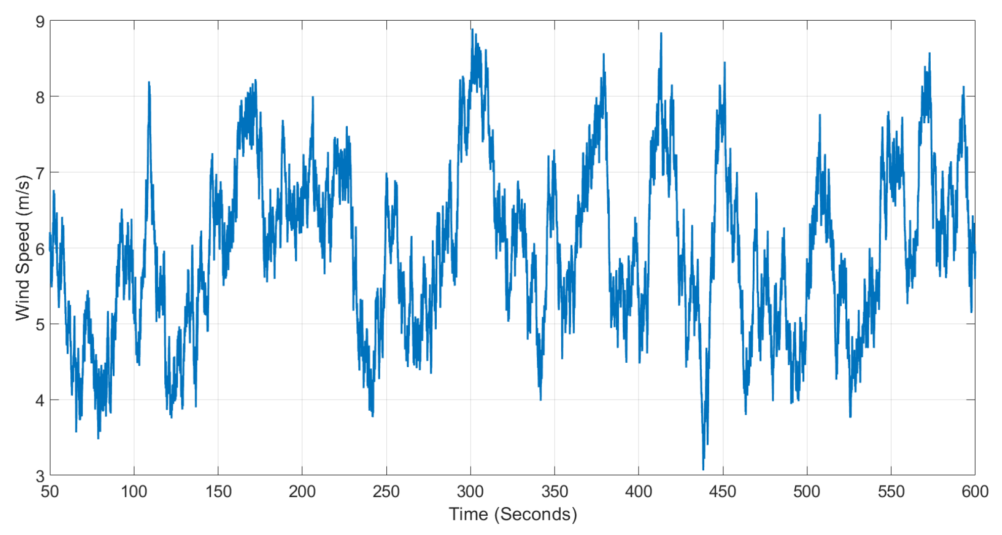
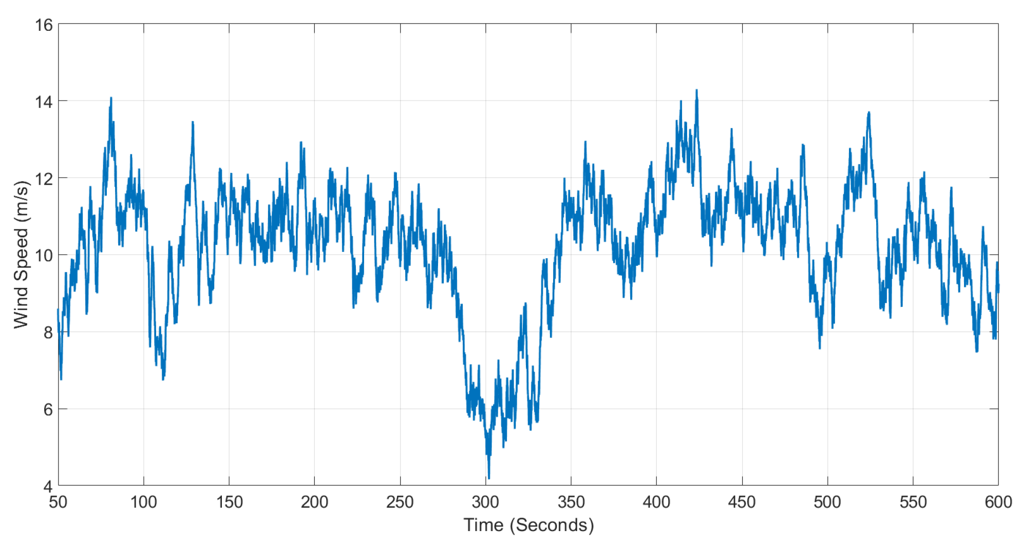
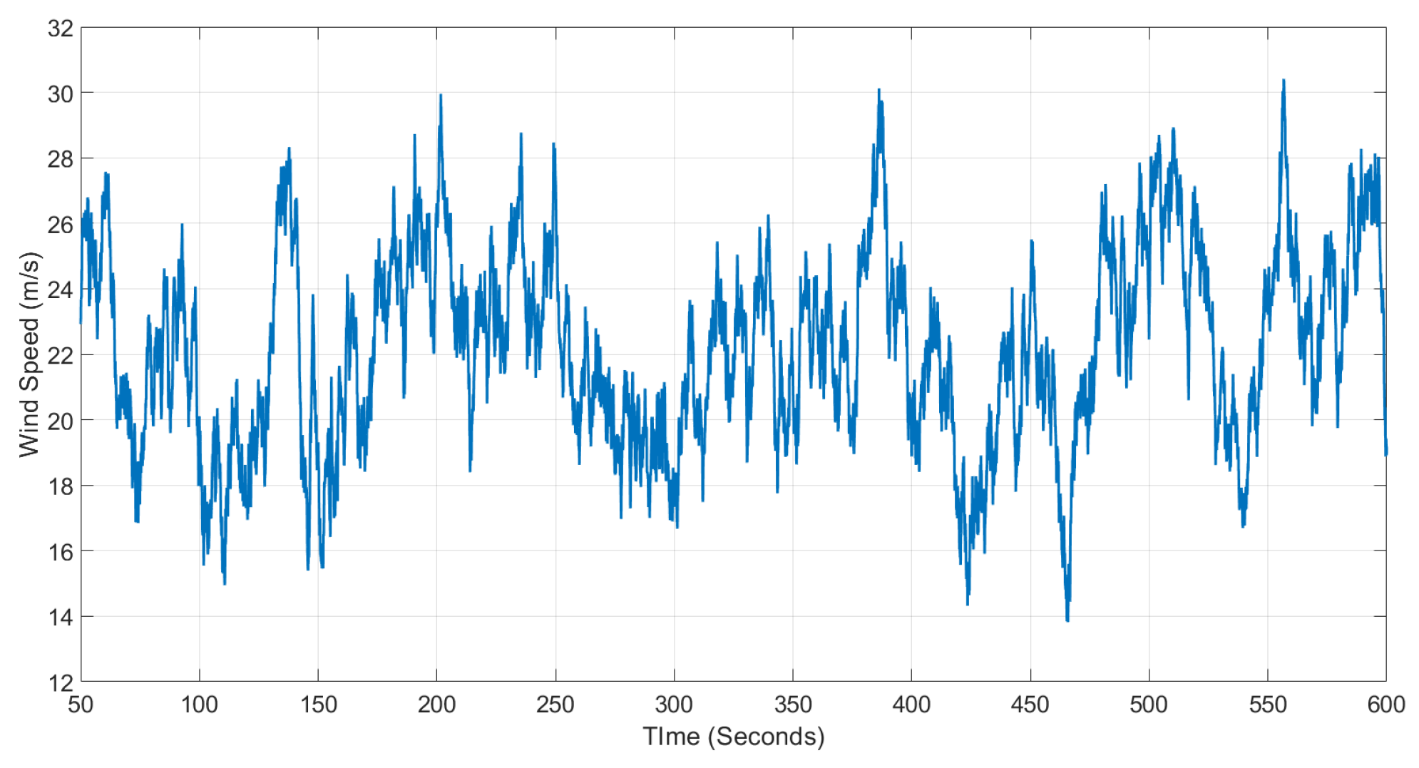
This section discuses the investigation of Scenarios 1 and 2 for the range of damage estimates discussed in Section 2.2.1. This is based on the use of the simulated wind turbine loads from a partly validated aeroelastic model of a widely commercial in-operation turbine, developed in Bladed software [18] (see Appendix A and [15] for more details). For the turbine loads simulation, the full operational envelope of mean wind speeds from the cut-in speed of 4 m/s, in increments of 2 m/s speed, up to the cut-out (24 m/s) has been considered. Examples of the hub wind speeds for a below-rated, close-to-rated and above-rated case are shown in Figure 3, Figure 4 and Figure 5, respectively.
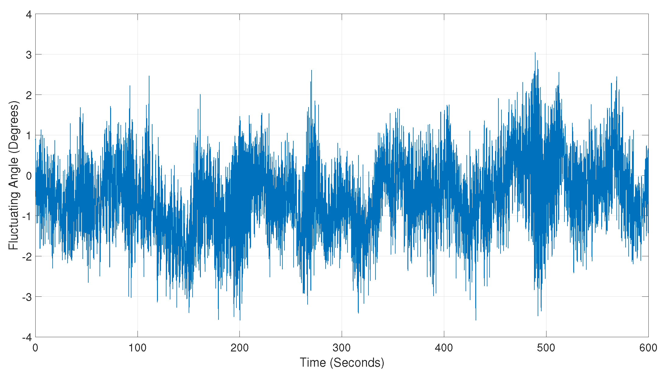
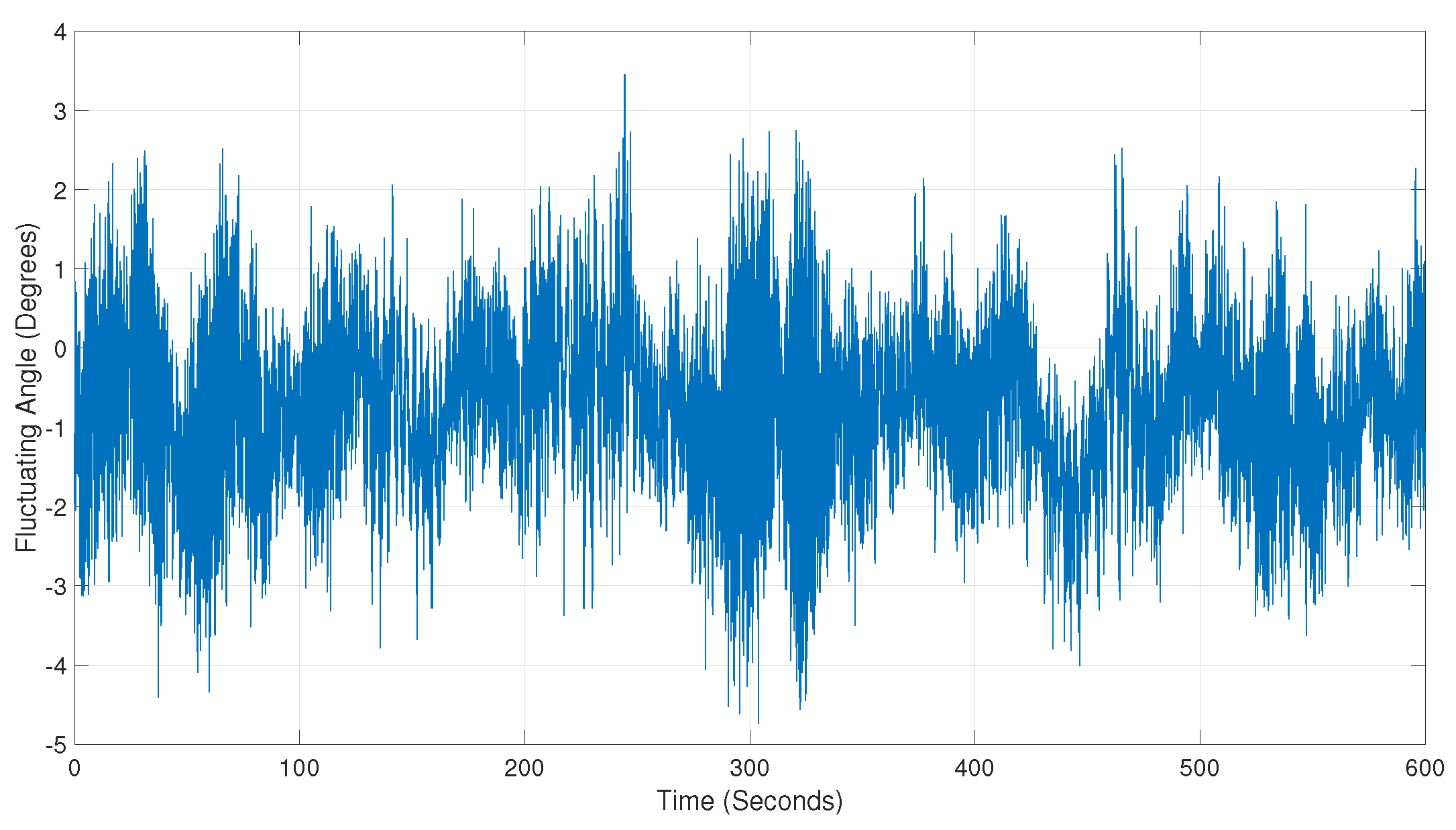
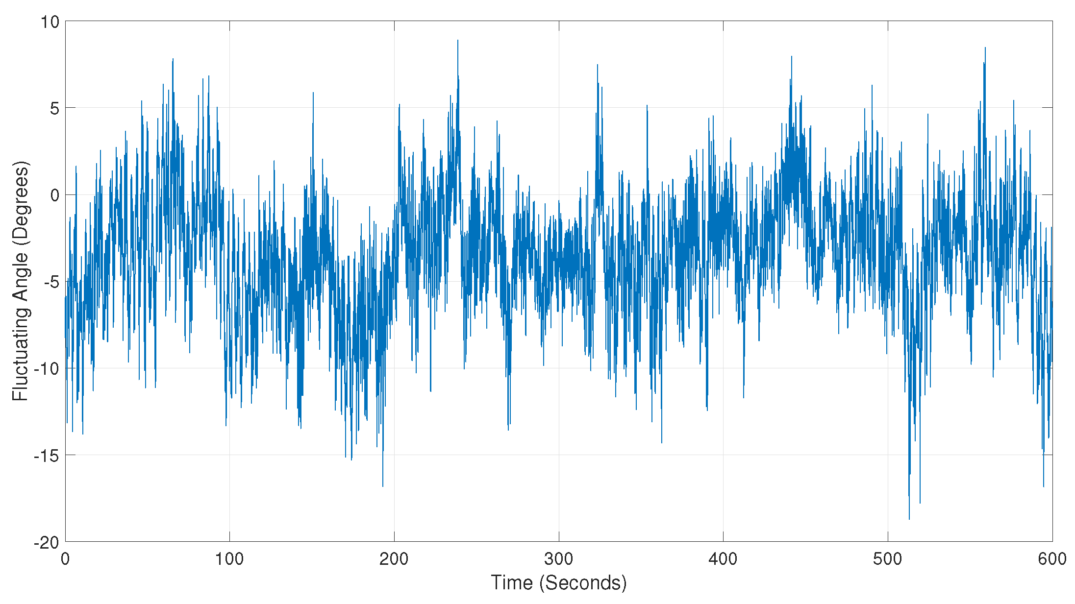
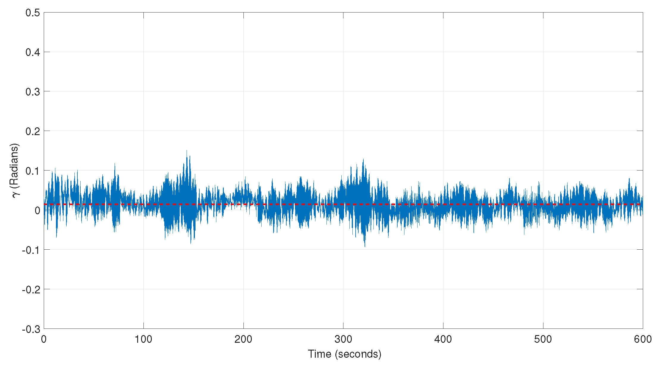
The fluctuating angle between the hub thrust and lateral forces, which are the main drivers of the tower loads (bending moments), and in turn, their fluctuations are also presented in Figure 6, Figure 7 and Figure 8, respectively.
For the fatigue damage accumulation and site-wide assessment of lifetime extension potential for different turbines (Section 4) the actual 10-minute average data are used. To this end, the mean wind speeds and directions are obtained from one year’s worth of data corresponding to seven turbines’ individual SCADA to derive the wind roses used within this section (partially provided in Appendix B). The first set of wind roses in Appendix B.1, is used for Scenario 1. The second set shown in Appendix B.2 is used for Scenario 2. The SCADA data are provided by the farm operator, and due to the commercial sensitivity, unfortunately, further information cannot be presented regarding the actual detail of the data sets.
3.2. Wind Turbine Case Study—Scenario 1
For Scenario 1, fatigue damage is determined using bending stress, . This bending stress is calculated using the resultant bending moment, M, and a cosine term, , therefore, demonstrates estimate (i) as discussed in Section 2.2.1. Afterwards, the influence of the deviation, , and the cosine term on the bending stress is investigated. The application of the Goodman’s correction factor is also considered. Approximate fatigue damage calculations using the resultant bending moment, M, and the fore-aft bending moment, , are also presented to demonstrate estimate (ii) and estimate (iii) as discussed in Section 2.2.1. The side-to-side bending moments, , and fore-aft bending moments, , for a range of mean wind speeds, v, are provided via the aeroelastic model (Appendix A and [15]). By combining the fatigue damage results with mean wind speed and mean wind directional probability, the influence of directionality on fatigue damage can be taken into account.
3.2.1. Impact of Deviation Angle on Tower Bending Stress and Damage
Firstly, it is worth investigating the change in the deviation angle, , used to calculate the bending stress. The value demonstrates how the ratio between side-to-side and fore-aft bending moment varies over different operation regimes.
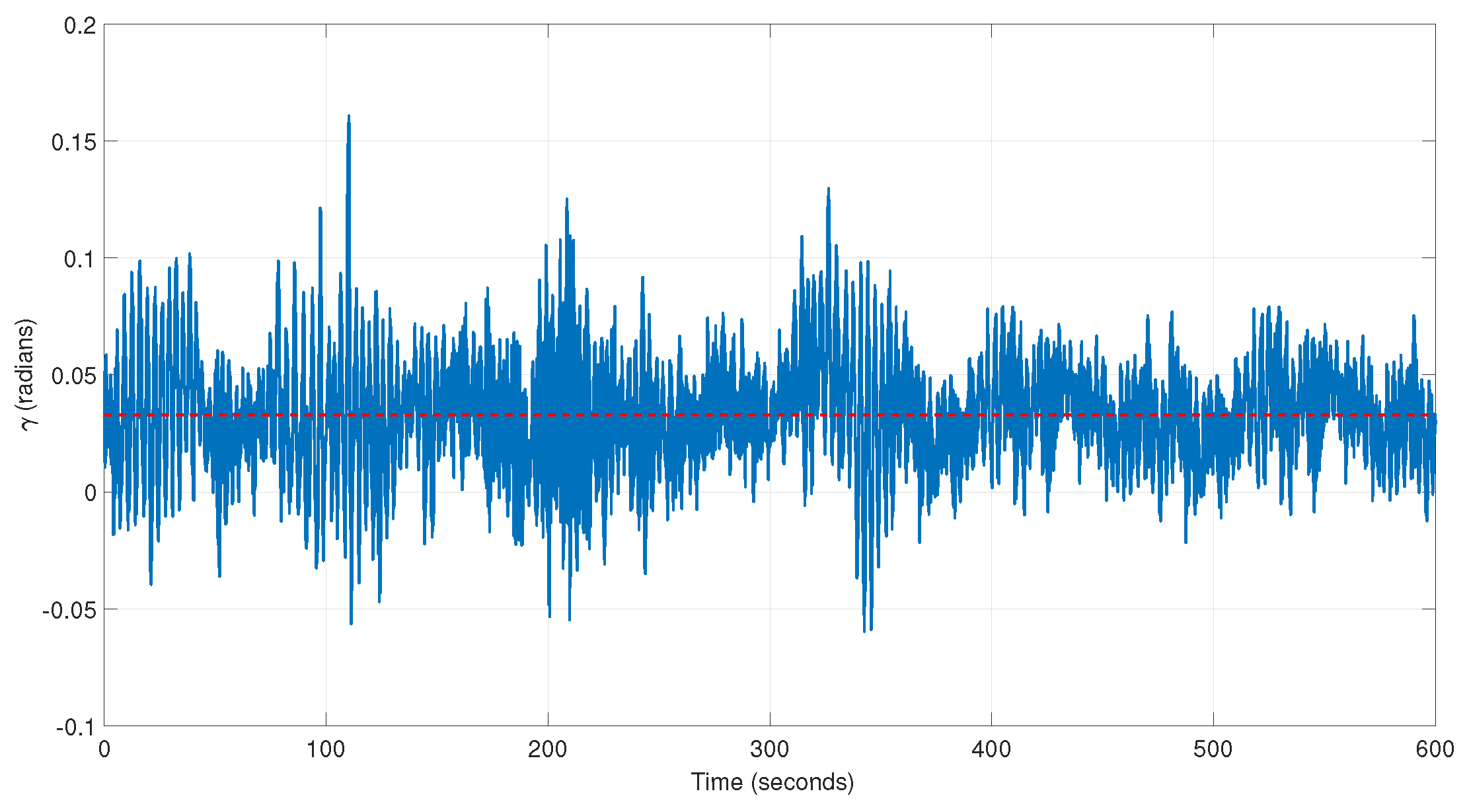
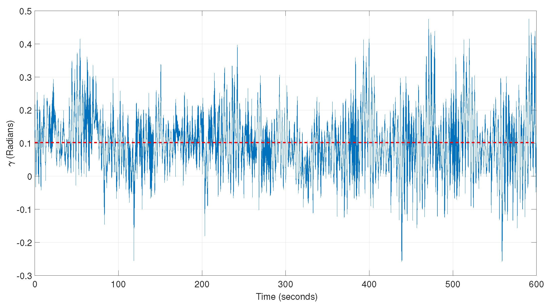
The values are calculated for a full range of operating mean wind speeds, and the results for a below-rated, rated and above-rated wind speed case, are shown in Figure 9, Figure 10 and Figure 11, respectively. The mean value of (shown as a red dashed line) for each mean wind speed increases from 0.015 rad (0.832) for a below-rated case, Figure 9, to 0.102 rad (5.845) for the above-rated case, Figure 11. The fluctuation also increases as the mean wind speed increases, significantly increasing the standard deviation.
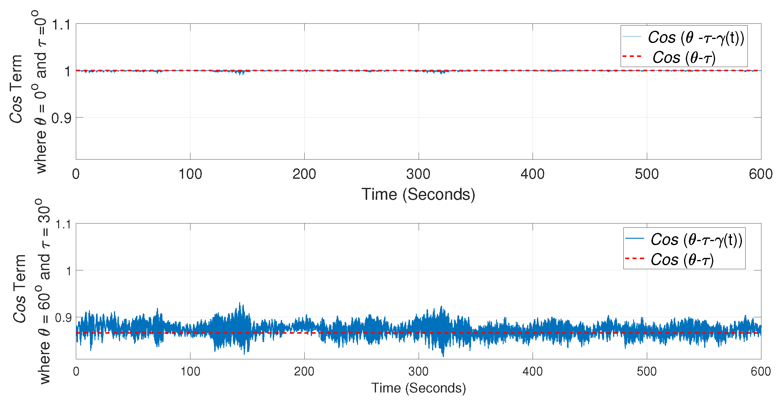
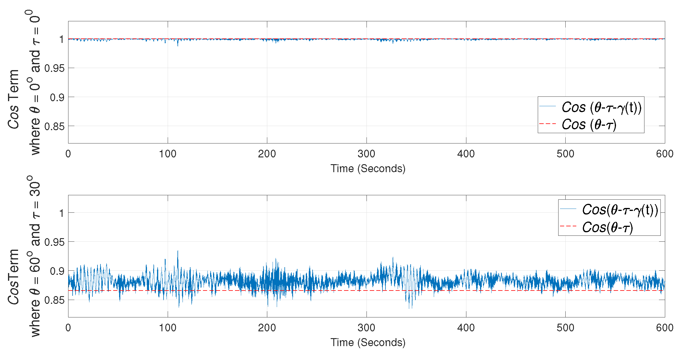
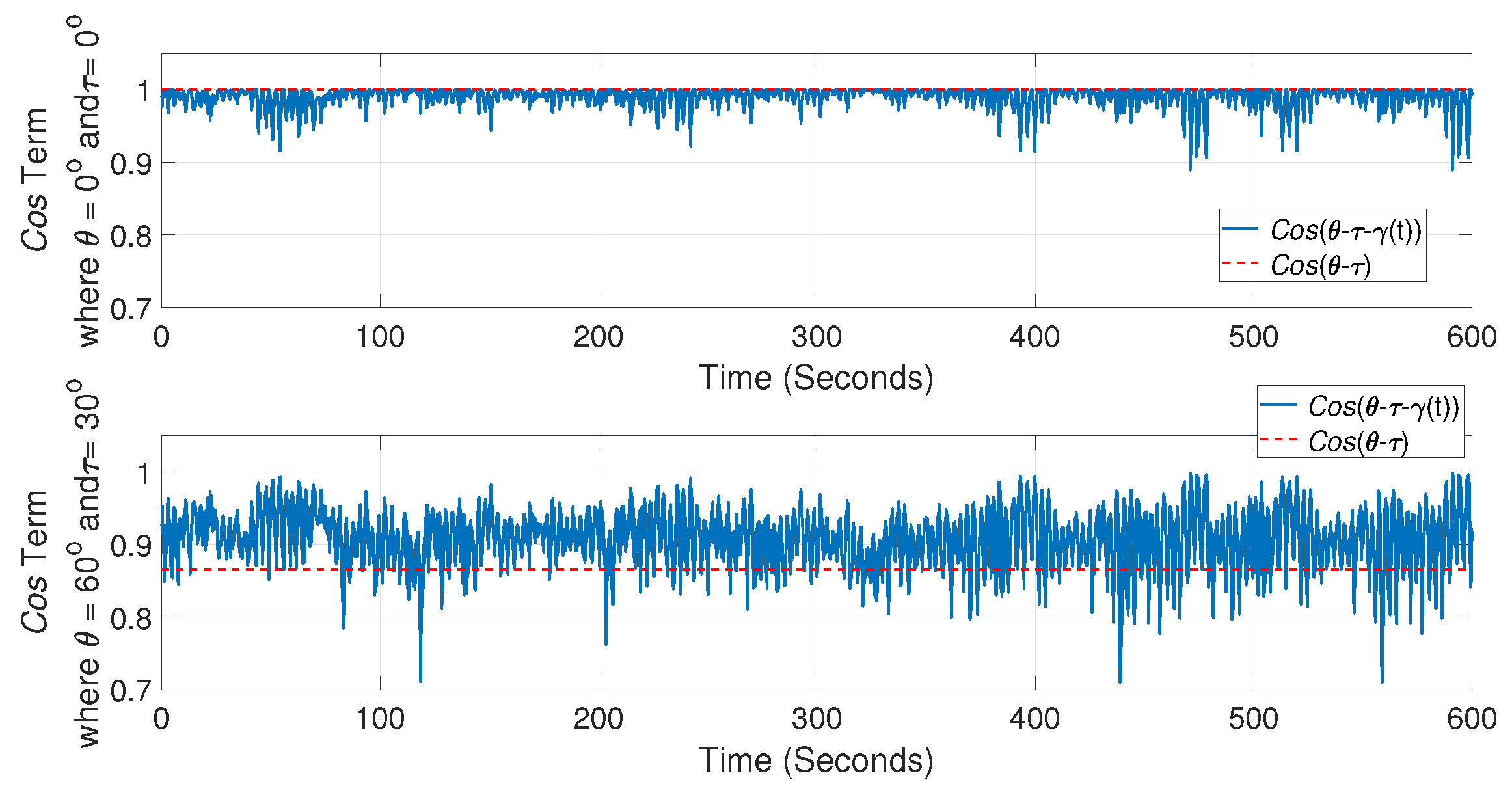
In order to calculate the bending stress within Scenario 1, , is calculated for the full range of tower positions, , and reference wind directions, . Again these are calculated for the full range of operating mean wind speeds. The results for the below-rated (6 m/s), close-to-rated power wind speed (10 m/s) and an above-rated case (22 m/s) are shown in Figure 12, Figure 13 and Figure 14 for fixed mean wind speeds and various and values (results provided for the estimates (i) and (ii)).
For the results set (the top graphs in Figure 12, Figure 13 and Figure 14), the cosine term is approximately 0.99 for a mean wind speed of 6, 10 and 22 m/s. On the other hand, for the results set (the bottom graphs in Figure 12, Figure 13 and Figure 14), the cosine term is, approximately, 0.86, 0.88 and 0.91, respectively, illustrating the difference between the results for the different mean wind speeds.
Calculations employing the resultant bending moment M and fore-aft bending moment only use , which is independent of time and only a function of tower position angle and wind speed direction. The results using this approximation of the cosine function are also shown in Figure 12, Figure 13 and Figure 14 as a red dashed line. As can be seen when and are 0 , the constant value cos( is closer to the accurate values, i.e., , which implies that has little impact. On the other hand, if and are not equal to 0, then the results of cos( are a poorer approximation to the full results. According to the results, the discrepancy between the approximated and accurate stress results increase when the difference between and , namely the angle between wind direction and the tower point for which damage is calculated, becomes larger.
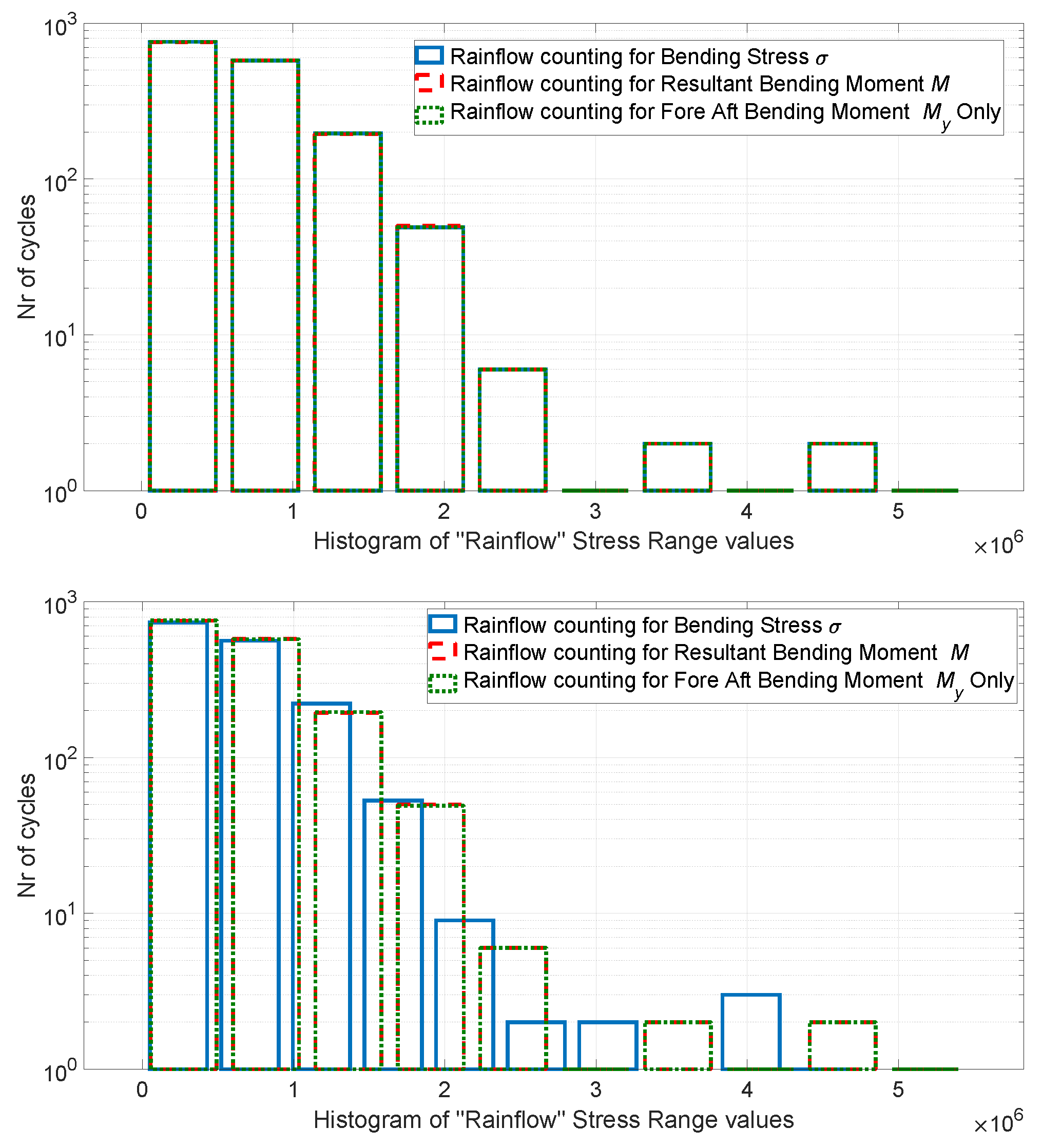
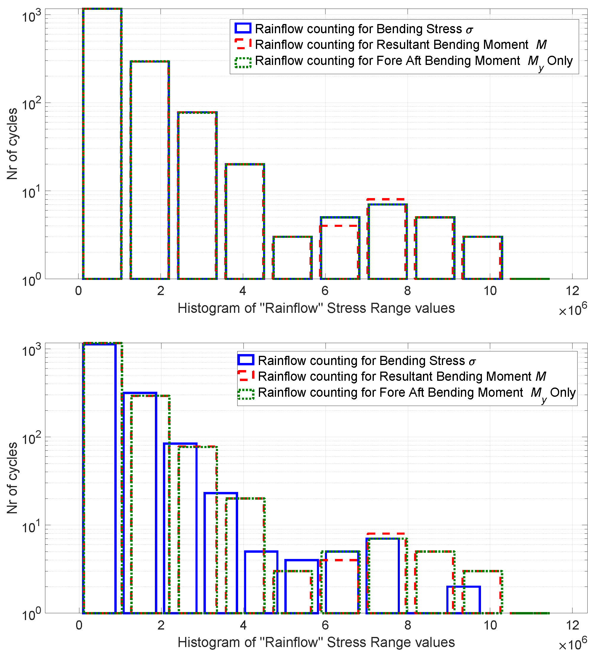
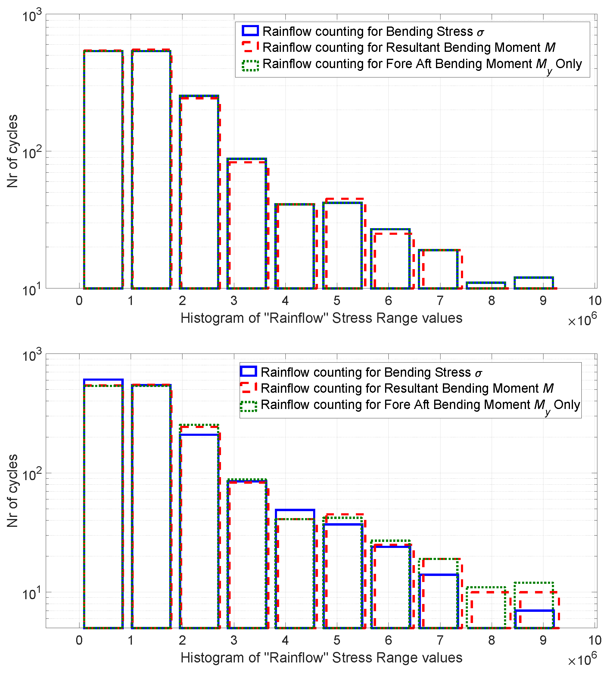
Rainflow cycle counting is used for fatigue damage calculations of 10-minute time series according to Equation (12) [21,22]. Figure 15, Figure 16 and Figure 17 show the results for cycle counting with tower section positions and , having values 0 and 0, respectively, (result set above) and with and equal to 60 and 30, respectively, (result set below).
According to Figure 15, Figure 16 and Figure 17, the difference between cycle counting histograms for the approximate and accurate stress time series increases with increasing wind speed and angle between the tower position and wind direction. It is important to note that this difference is not only observed in the number of cycles but the stress ranges. The difference in the number of cycles and stress ranges between the approximate and accurate stress results when and are both equal to 0 is not significant as can be seen in the top plots in Figure 15, Figure 16 and Figure 17. On the other hand, when is 60 and is 30 , there are observable differences between the results for the approximate and accurate stress time series. For the below-rated in the bottom of Figure 15, there is a considerable difference in the stress ranges. In the rated case, the bottom plot in Figure 16, the number of cycles especially at the lower stress range has increased for the approximate results, and the values of each stress range have decreased slightly. For the above-rated case, in the bottom plot in Figure 17, there is less difference in stress range values between the approximate and accurate stress results, but there is an increase in the number of cycles for the approximate results compared to the accurate case. Moreover, this difference cannot be resolved solely by inclusion of the side-to-side bending moment, namely using the resultant bending moment. The deviation angle, , has to be taken into account too.
3.2.2. Influence of Wind Rose Probability (Directionality Effect)
The closed form solution shown in Equation (1) consists of two terms. The damage term has been discussed earlier in this section. The second term takes into account the wind speed and wind direction through wind rose data. The best way in which to identify the influence of the wind directionality on total damage is through the calculation of the .
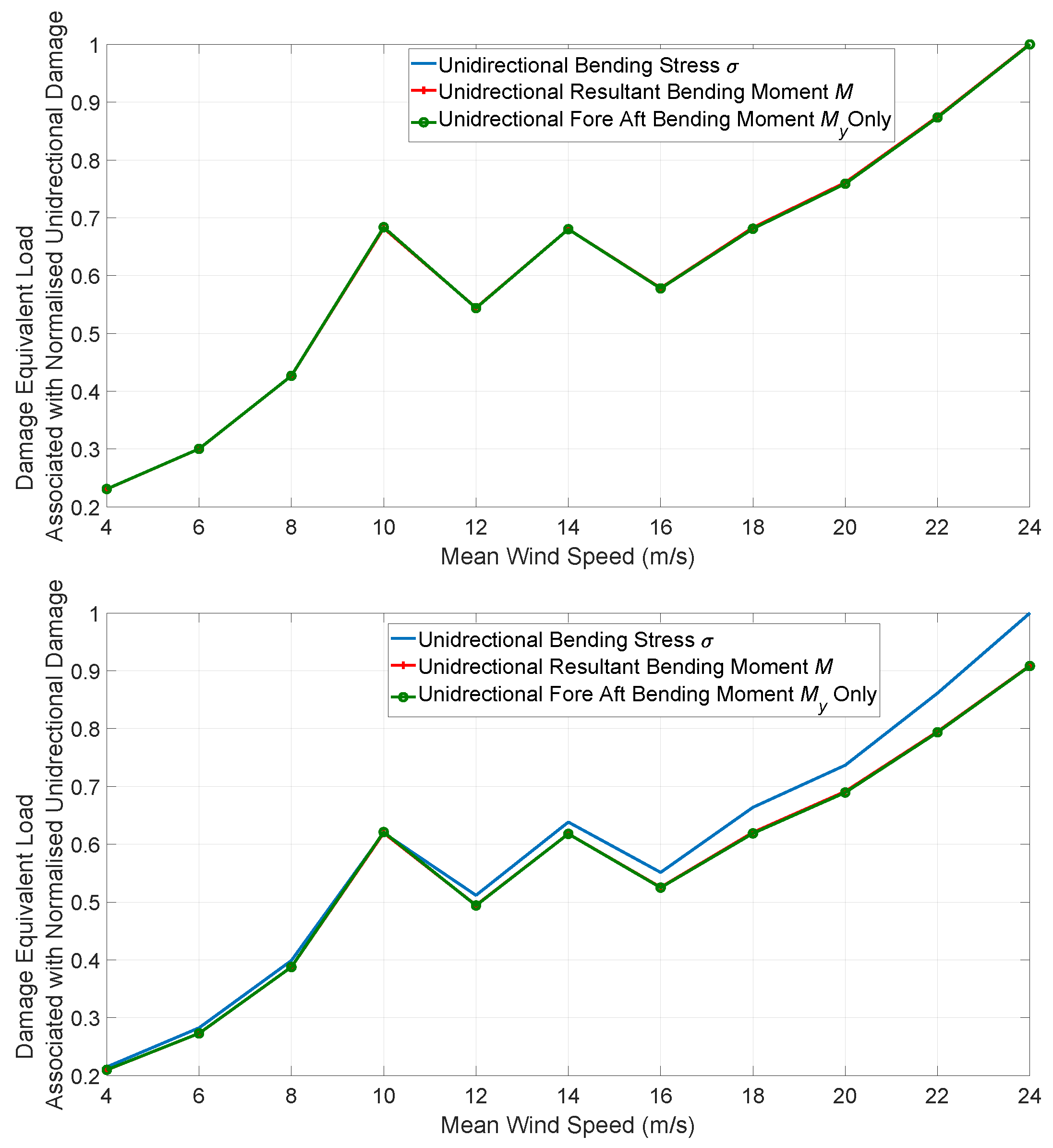
In order to calculate the uni-directional fatigue, a modified version of Equation (12) is used. Note that the uni-directional damage merely includes the damage contribution associated with the wind blowing from a fixed direction; therefore, is set to 1. Results in terms of damage equivalent loads (DELs) are shown in Figure 18, where the values have been normalised around the maximum fatigue damage due to bending moment stress at 24 m/s. This is to easily demonstrate the trend in fatigue damage across the range of mean wind speeds.
For the result set where and both have values of 0 , the results for normalised DELs of uni-directional damage using the bending stress, , resultant bending moment, M, and fore-aft bending moment, , are shown in the top of Figure 18. In this case, all the wind is assumed to be coming from the reference wind direction, , of 0 , causing damage to the tower at position of 0 . For the results set where and are 60 and 30 , respectively, the results for directional damage using the bending stress , resultant bending moment, M, and fore-aft bending moment, , are shown in the bottom of Figure 18. In this case, there is a 30- shift between wind direction and tower position.
As can be seen in Figure 18, the normalised DELs of uni-directional wind generally increase with mean wind speed, v, as expected. For the results set in which and have values of 0 , there is no significant difference between the accurate DELs calculated using bending stress, , and the approximations using resultant bending moment, M, and fore-aft bending moment,, for the full range of mean wind speeds, see the top of Figure 18. However, for the results set where and have values 60 and 30 respectively, there are deviations of the resultant bending moment, M, and fore-aft bending moment, , from those using bending stress, which increases in parallel with wind speed going up. There are some variations in this trend about the rated speed (10 m/s), which is likely due to the change in the operations regime and switching between below-rated and above-rated control.
As stated previously, according to design standards, the wind turbine towers have to withstand the worst-case load. Here, the worst-case load is taken to be the uni-directional load, where all the wind coming from a single direction is acting on the point on the wind turbine towers circumference, which undergoes the highest damage. As such, it is common practice to assume that the point with the largest damage lies on the axis of wind direction distanced from a neutral axis equal to the tower radius. This corresponds to setting in the closed-form solution to calculate the worse case scenario or uni-directional damage and is taken as the design reference damage in the rest of this study.
When the Goodman’s correction Equation (13) based on the evaluation of is applied, the uni-directional fatigue damage and associated damage equivalent load is significantly higher, as can be seen in Figure 19, as the mean bending stress remains tensile. The trend is similar to that of Figure 18. The deviations from the generally increasing trend between 8 and 16 m/s seen in Figure 18 are larger, emphasising greater fatigue damage induced when the tower is in tension by taking into account the mean stress effects.
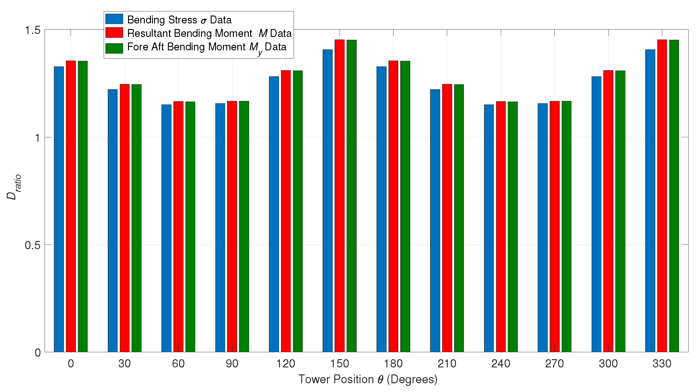
Next, for each value of , corresponding to the tower positions, the fatigue damage from each value is accumulated across all wind speeds, v, using the closed form solution to obtain the damage ratio, , by Equation (14). This damage is referred to as multi-directional damage. Here, the baseline uni-directional damage for evaluation of the damage ratio corresponds to the wind turbine (wind rose) 7 (Figure A4), as also used in Section 2.2.1. In this example, wind rose 1 (Figure A2) is used for taking the joint probability values of mean wind in 30 bins and the wind speed between 4 and 24 m/s in 2 m/s bins. Note that wind rose 1 and 7 belong to the actual turbine across a wind farm. The results of damage ratios on different tower positions are given in Figure 20.
Since tension or compression has not been considered, there is assumed symmetry around the tower, as can be seen in Figure 20. The maximum fatigue damage would lead to the smallest value; therefore, due to the assumed symmetry, this critical point occurs at a tower position, , of 60 and 240 for wind rose 1 (see Figure 20). Figure 20 also demonstrates the underestimation of fatigue damage using the approximations compared to the accurate calculations.
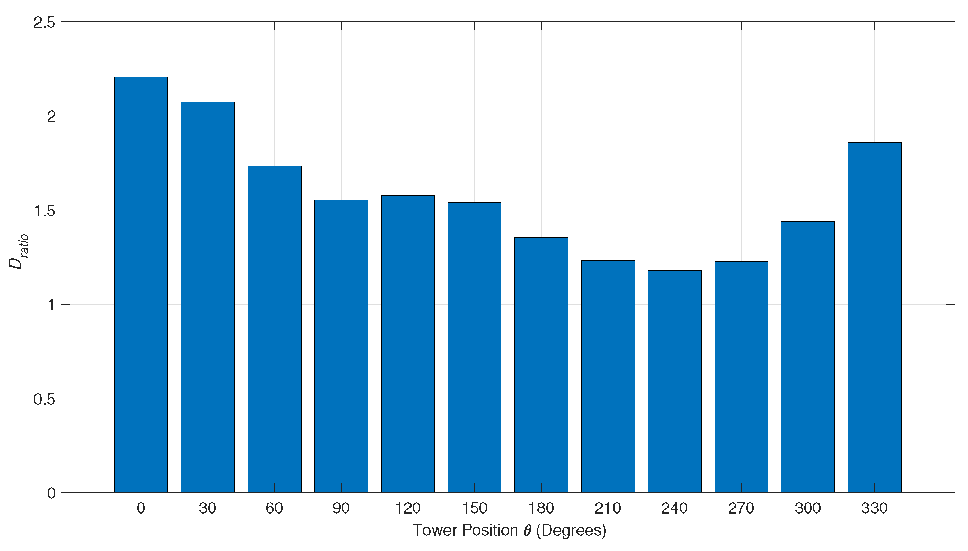
The same procedure is then carried out using bending stress only, but in this case, the uni-directional damage corresponding to wind rose 7 (Figure A4) is calculated with the application of the Goodman’s correction factor, as discussed in Section 2.2.1. The values are taken as the fatigue damage calculated for each tower position, , with the application of the Goodman’s correction factor. The results for wind rose 1 (Figure A2) with the application of the Goodman’s correction factor are shown in Figure 21.
The symmetry noted previously in this section no longer applies, and the damage equivalent load is different at each value. The maximum fatigue damage would again lead to the smallest value; therefore, this critical point occurs at a tower position, , of 240 for wind rose 1 (see Figure 21).
3.3. Wind Turbine Case Study—Scenario 2
As stated previously, it can be the case that only wind roses are available, e.g., from turbine SCADA data. Using a slight modification of Equation (12), an estimation of the directional fatigue damage or damage equivalent load using mean wind speed and mean wind direction probabilities can be made. For this scenario, the results of are replaced with the generic fatigue damage or damage equivalent load, , for each mean wind speed, v, and the cosine term reduced to . The probability values of and are now independent values, therefore demonstrating estimate (iv), as discussed in Section 2.2.1.
In this case, three wind roses shown in Appendix B are used. Wind rose A, (Figure A5) shows a hypothetical equally distributed wind rose. Wind rose B, (Figure A6) and C, (Figure A7) are roughly based on generic wind rose data with prevailing wind directions in higher wind speeds.
Again, to identify the influence of the wind directionality on fatigue damage, it is studied through the calculation of the , as discussed in Section 3.2.2. Therefore, uni-directional damage, and a maximum damage from multi-directional damage need to be calculated again.
3.3.1. Uni-Directional Fatigue Damage
As with scenario 2, the fatigue damage or damage equivalent load, , is multiplied by equal to 1 and uses result set i where and are both 0 . A very similar result to Figure 18 is produced. The damage increases with mean wind speed, v, and there is some fluctuation around mean wind speeds. The proxy Weibull distribution is calculated and multiplied by this fatigue damage. It should be noted that Wind Rose A, the equally distributed wind rose, is only equally distributed in terms of mean wind direction and not mean wind speed; therefore, will still have a proxy Weibull distribution. The final direct damage is calculated by summing the damage across the mean wind speeds. Finally, the results of fatigue damage calculated above are multiplied by the proxy Weibull distribution and the total uni-directional damage calculated by summing the damage across each mean wind speed.
3.3.2. Multi-Directional Fatigue Damage
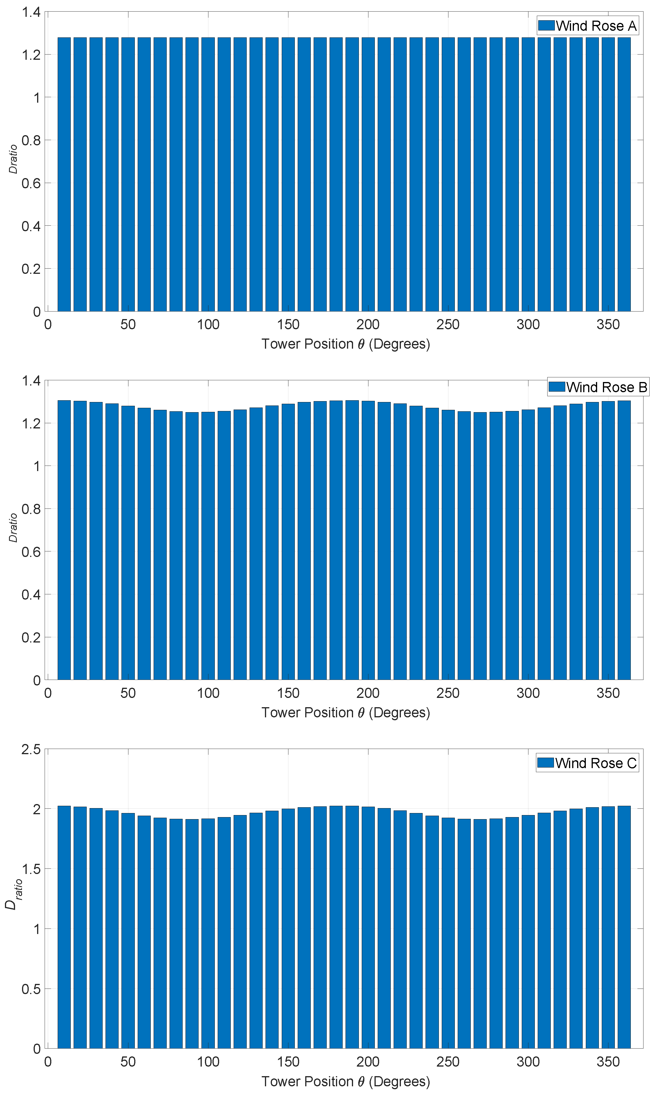
In a similar manner to scenario 2, for each value of the fatigue damage from each value is accumulated across all wind speeds, v, using the modified closed form solution. In order to calculate the , the maximum fatigue damage is taken as the fatigue damage calculated for each tower position, , and is taken as the uni-directional damage calculated for each of the respective wind roses. The results of these calculations using the equally distributed wind rose for the uni-directional wind, are shown in Figure 22.
The assumed symmetry around the tower can again be seen in Figure 22. For wind rose A, the equally distributed wind rose, the value is constant across all tower positions, , as expected due to the equal distribution of wind direction. For wind rose B and C, there is variation in the value. For wind rose B, the critical point with the maximum fatigue damage occurs at a tower position at 80 and 260 and for wind rose C at a tower position of 70 and 250 .
Later, within the subsequent section, the impact of the defined scenarios and their combinations with the sets of estimates i–iv are closely studied for a wind farm case study to evaluate the turbines’ potential for lifetime extension.
4. Wind Farm Case Study
4.1. Data
This section uses the same wind speed data and, hence, bending moment data as discussed in Section 3.1. The wind roses are again those discussed in Section 3.1, which correspond to the individual turbines.
4.2. Case Study Description
The context for this paper considers the practical evaluation of the potential for life extension of turbines in a wind farm when varied levels of data/information on the turbine load and wind are available. Therefore, a case study has been used to demonstrate how the closed form solution can be applied to a range of scenarios. These scenarios were discussed in Section 2.2.1. Estimates (i)–(iii) are suitable for scenarios 1, whereas (iv) is suitable for all scenarios. Although much cruder, (iv) can still provide useful information as to what turbines have the greatest potential. Note that it provides a limit for the maximum life extension relative to uni-directional wind speed but does not take into account whether the conditions for a particular turbine are more or less benign.
In a similar manner to the wind turbine case study in Section 3, it is assumed that the bending moment data are only available for one wind turbine within the wind farm. For Scenario 1, the associated bending stress, , resultant bending moment, M, fore-aft bending moment, and wind rose data are available [15]. The wind farm in which these turbines are operating is located in the Scottish Highlands. To inspect the site-wide variation in the fatigue life analysis results, the turbines are purposely selected from different locations across the farm. All the machine or farm details cannot be disclosed due to confidentiality restrictions, but the essential information for the purpose of the current study is provided in Appendix A with individual turbines’ wind rose data in Appendix B. Firstly, the side-side bending moments, , and fore-aft bending moments for a range of mean wind speeds, v, are used and the wind roses are again those discussed and partially shown in Appendix B.1.
4.3. Case Study Results
The fatigue damage for the first scenario, where only one set of bending moment data was available for one turbine and wind roses were available for all wind turbines under investigation, is calculated using bending stress, , resultant bending moment, M and fore-aft bending moment, using the methodology presented in Section 2 and Section 3.2. This section presents the results for calculating the final values, and ultimately, the lifetime extension potential of the selected wind turbines from the wind farm case study.
The different headings for each set of results and there description is as follows:
- Bending Stress —These results investigate Scenario 1 for estimate (i).
- Bending Stress with Goodman’s correction—These results investigate Scenario 1 for estimate (i) with additional calculations to take into account tension and compression.
- Resultant Bending Moment M—These results investigate Scenario 1 for estimate (ii).
- Fore-aft Bending Moment —These results investigate Scenario 1 for estimate (iii).
- Normalised Wind Rose—These results investigate Scenario 2 for estimate (iv).
- Finite Element Analysis—Results calculated using finite element model for stress analysis are included for comparison and validation of the above sets of results [15].
The absolute had already been established for each tower position, , for each wind rose, as discussed in Section 3.2 and Section 3.3. This process allows the associated with the critical point with the maximum damage to be identified. In all scenarios, the uni-directional damage is taken as the direct damage calculated using wind rose 7 (Figure A4). The uni-directional damage or damage equivalent load for any other turbines could be adopted, however, as long as the uni-directional damage is the same for all turbines for all comparisons.
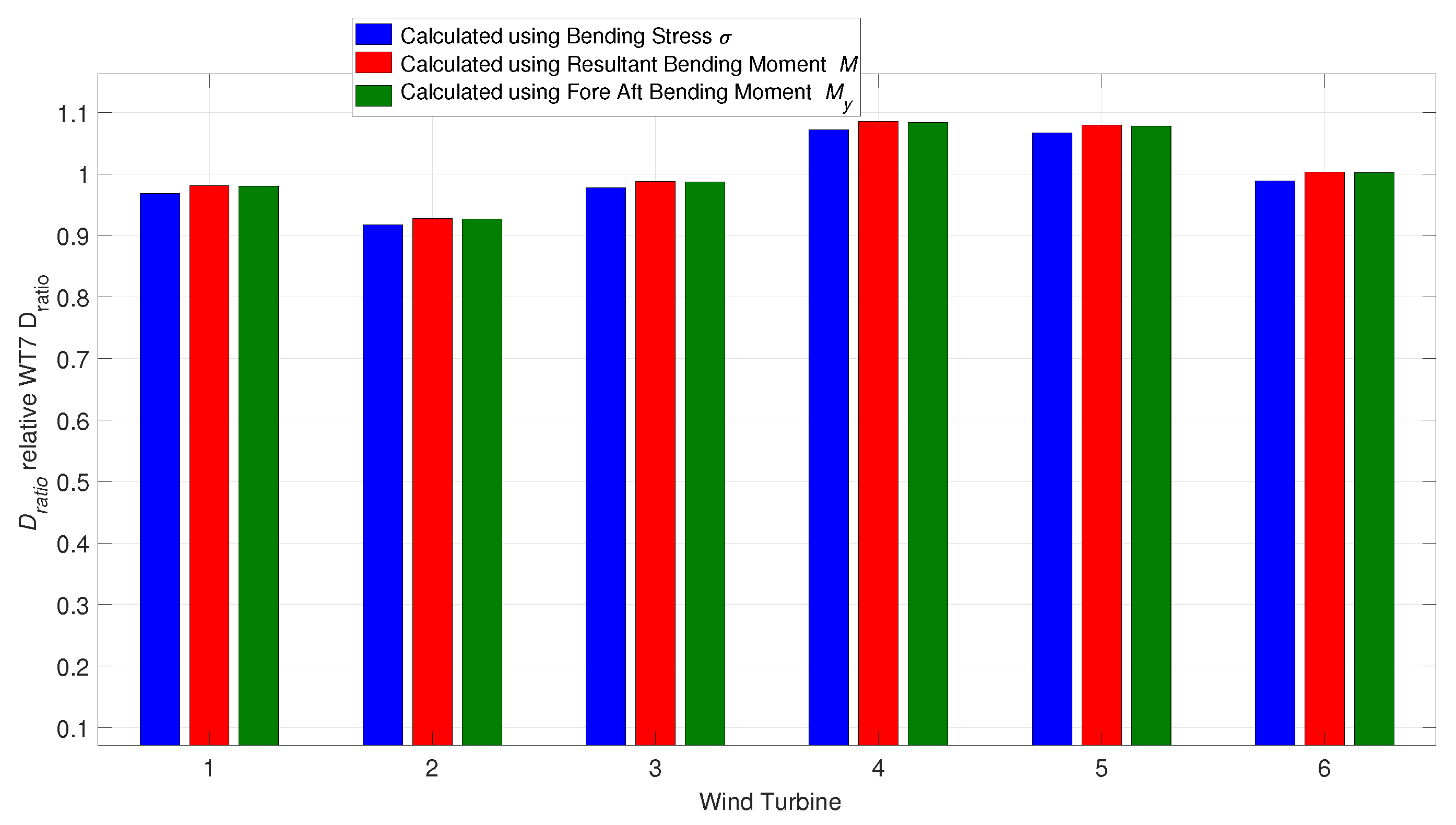
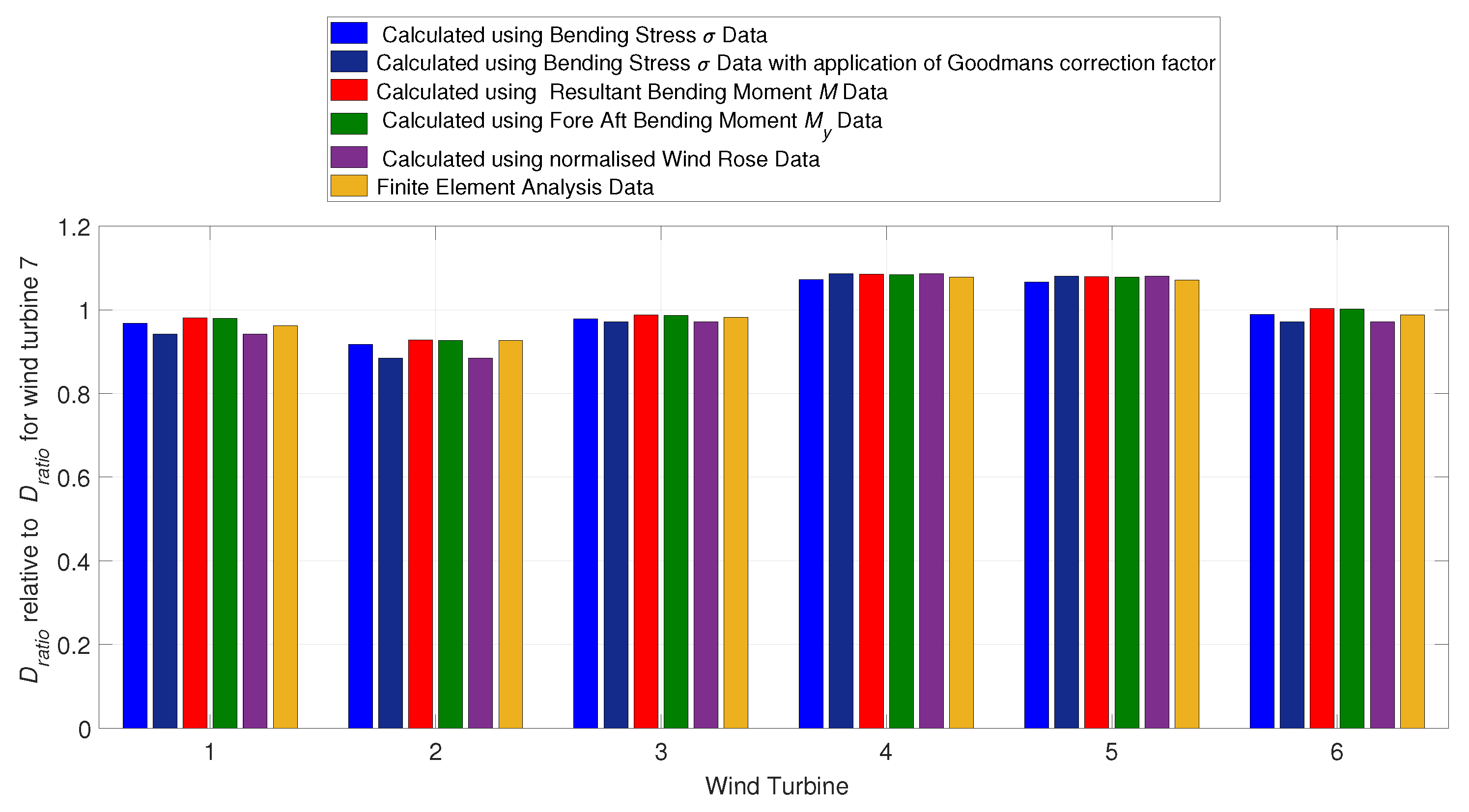
Firstly, the relative results of Scenario 1, using the bending stress, , the resultant bending moment, M, and fore-aft bending moment, , are presented in Figure 23. Note that for ease of comparison, the results have been normalised relative to turbine 7’s bending stress damage. In many cases when investigating wind turbine tower fatigue only fore-aft, , bending moment data is representative for design or control strategy optimisation. Comparison between the results using the bending stress, , the resultant bending moment, M, and fore-aft bending moment, , can indicate whether using just would provide suitable results. Figure 23 shows the normalised values in Scenario 1.
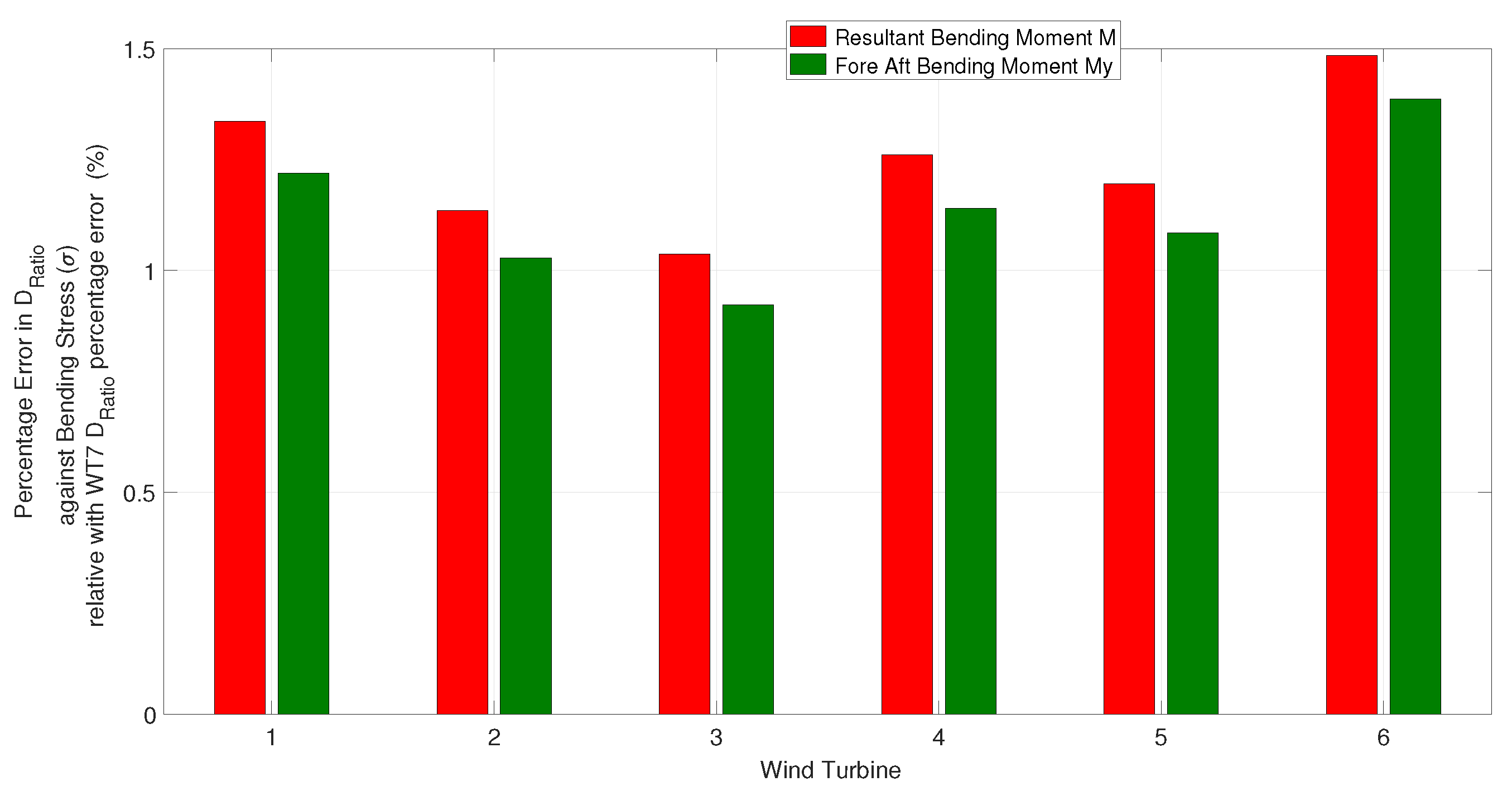
The percentage differences between the estimates for the relative ratio, , using the resultant bending moment, M, and the fore-aft bending moment, , relative to the relative estimates using the bending stress, , are shown in Figure 24.
As can be seen in Figure 23, there is no significant difference between the results calculated using bending stress, , resultant bending moment, M, and fore-aft bending moment, . The percentage differences between normalised results shown in Figure 24 are approximately ranging between 1 and 1.5 % for M and 0.9 and 1.4 for . Both sets of results are expected since the uni-directional damage or DEL is calculated with a fixed value of 0 for both and , and there is very little difference between the normalised uni-directional damage or DEL, as shown in Figure 18. This error is not specific to uni-directional damage, as it also appears in the multi-directional wind damage calculations too.
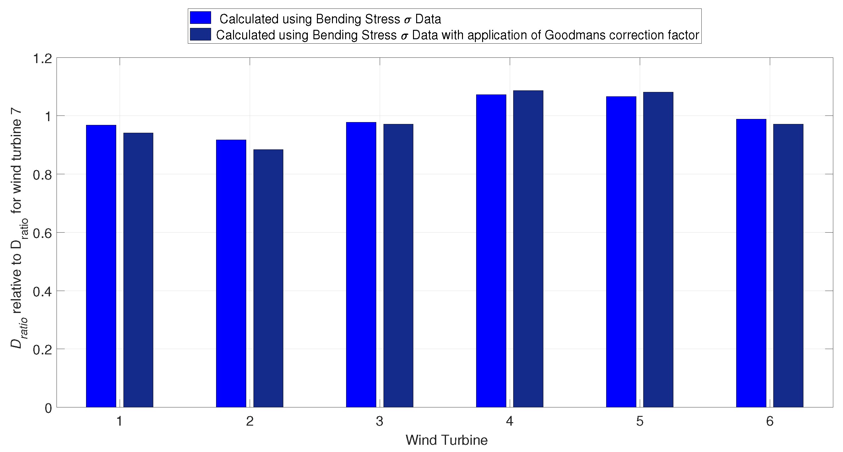
The results for the range of wind turbines using bending stress with and without the application of the Goodman’s correction factor are shown in Figure 25. It indicates that wind turbines 1, 2, 3, 6 have more tensile loads, which leads to higher fatigue damage or DEL since the reduces when Goodman’s mean stress correction is applied. On the other hand, there is the opposite situation for wind turbines 4 and 5. Overall, however, there is very little difference in the results when applying the Goodman’s correction, and similarly, when using resultant bending moment, M, and fore-aft bending moment, , very little difference is expected. Therefore, due to the small difference, the rest of those results were not considered.
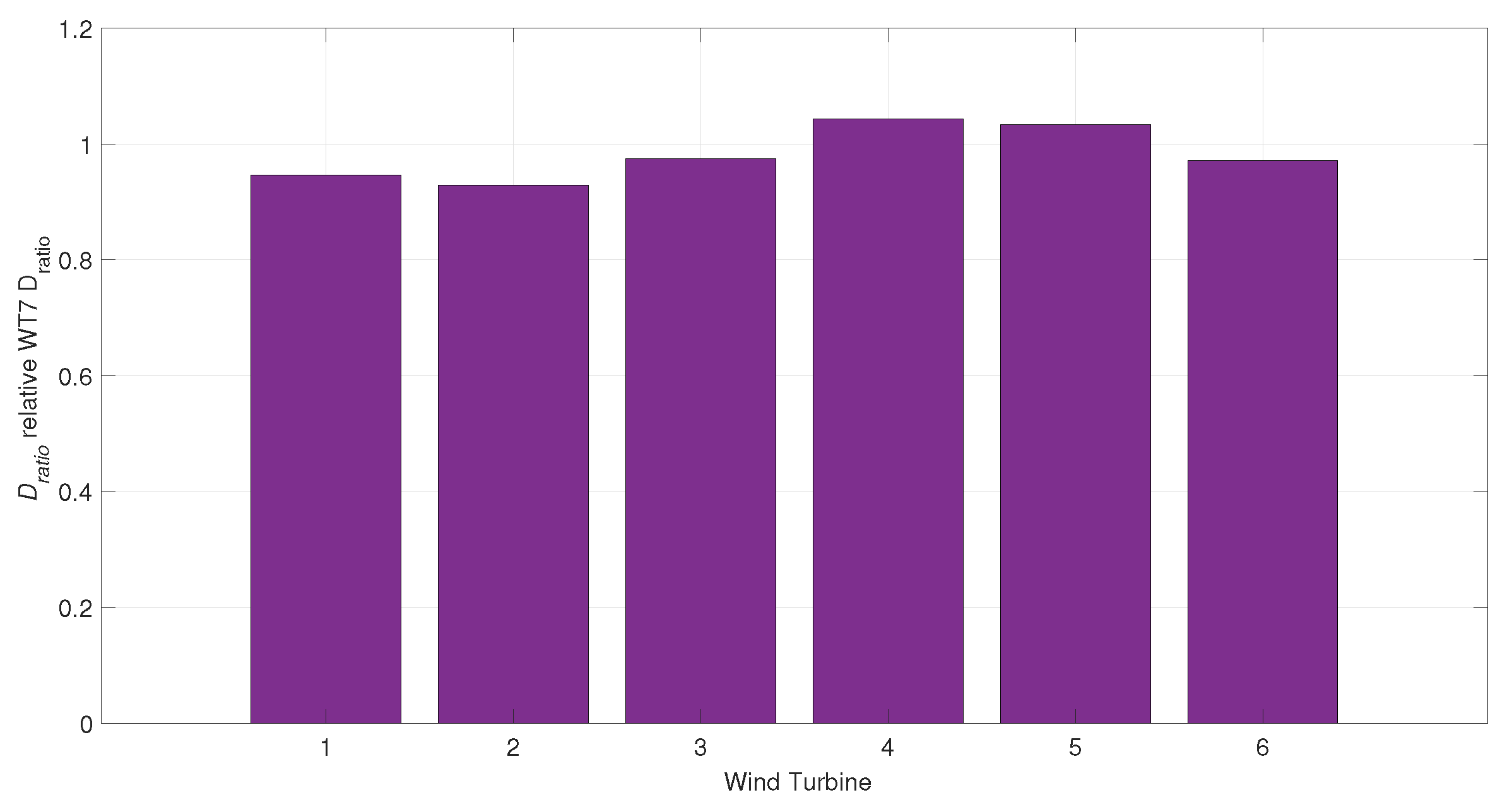
Finally, the results using just the wind rose data are shown in Figure 26. The results shown in Figure 26 indicate that the for wind turbine 2 is the smallest, indicating the largest fatigue damage relative to the ratio for wind turbine 7, and wind turbine 4 has the highest indicating the smallest fatigue damage relative to the ratio for wind turbine 7.
4.4. Comparison and Discussion for Wind Farm Case Study
In order to cross-check the presented damage ration results, a comparison is made between the values for each scenario and the corresponding calculated using the finite element (FE) analysis results by Kazemi Amiri et al. (see [15] for more details on the FE analysis).
The results shown in Figure 27 combine the results from Figure 23, Figure 25 and Figure 26 together with the above-mentioned FE analysis results from [15]. The figure shows that although there are some small variations in the magnitudes, in each case, the trend for is the same. The lowest relative and, therefore, highest relative damage occurs for wind turbine 2, and the highest relative and, therefore, lowest relative damage occurs for wind turbine 4. There is little difference between the results using bending stress, , resultant bending moment, M, and fore-aft bending moment, , and the inclusion of the Goodman’s correction factor has had little impact. The results from the wind rose only scenario are comparable but do include some over- and underestimations due to the intrinsic approximation.
The aim of the investigation is to identify the wind turbines that have the greatest potential for lifetime extension, which can be identified from the trends rather than the specific values. Since the wind rose only case exhibits the same trends, then the wind rose only case can clearly be used as an acceptable indicator of life extension potential once the wind direction effect is taken into account. Additionally, Figure 27 shows that the values for each case are comparable with the finite element analysis results, which successfully demonstrates the results’ cross-check.
4.5. Lifetime Extension Potential
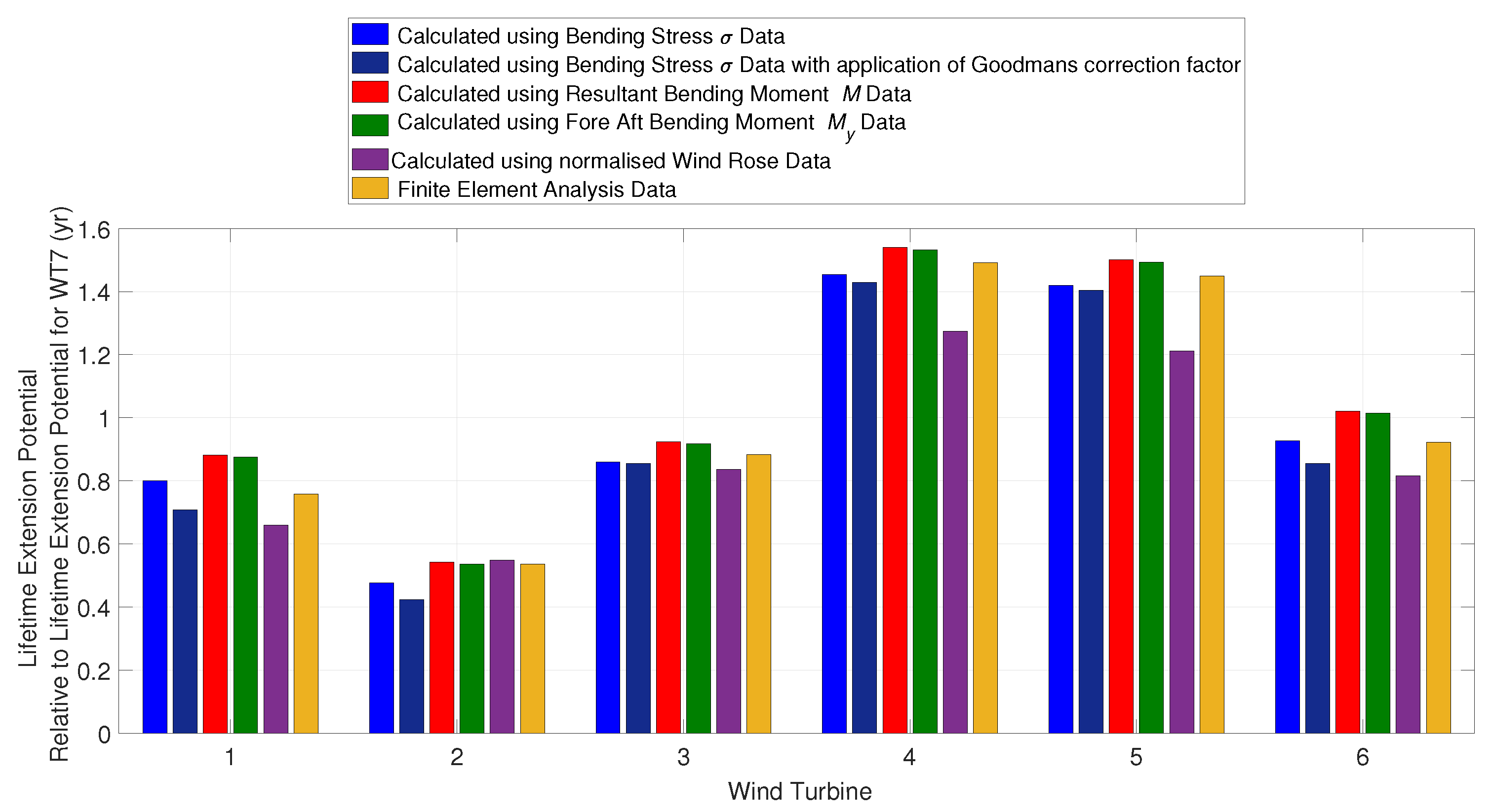
Finally, the turbines’ indicators for lifetime extension potential () are calculated relative to the arbitrary representative turbine’s (number 7) damage using bending stress data and are presented in Figure 28.
As expected, the wind turbines with the lower values have the least potential for lifetime extension whereas those with larger values such as wind turbine 4 have the highest potential for lifetime extension. It is not very sensible to speak about the actual extra life in years, so long as a detailed life extension analysis for turbine 7 has not been performed. However, the relative lifetime extension potential values indicate that for instance, turbine 4 has greater than 1.4 times longer life relative to wind turbine 7’s life determined from its bending stress based on 1 years worth of data. On the other hand, for wind turbine 2, the extended life is less than 60% of that of turbine 7. The lifetime extension potential calculated using just the wind rose data clearly has different values from the results calculated using bending stress, , resultant bending moment, M, and fore-aft bending moment, . The trend is, however, the same, and therefore, an acceptable prediction can be made. Figure 28 also shows the fact that when tensile or compressive loads are considered using the Goodman’s correction factor, this has an impact on the lifetime extension potential, for example, wind turbine 2 identified as having larger tensile damage with higher damage leads to a lower potential for lifetime extension. Nevertheless, it is notable that this impact does not alter the trend of relative lifetime extension potential results across different turbines.
Inspecting Figure 28 clearly indicates that the relative lifetime extension potential values vary more significantly among different sets of estimates than the normalised damage ratios. Although, a good trend of the estimated extended life can be obtained, e.g., from wind roses only. However, the results are based on which mostly show underestimation of the relative potential lifetime extension, significantly deviating from those obtained through other methods for some of the turbine across the farm. Hence, the large variation of the relative potential extended life using different approximations (Table 1) emphasises the fact that the accurate estimation of turbines remaining useful life is crucially important, given the fact the extended life will be just a fraction of the turbine’s design life.
5. Conclusions
A methodology to evaluate the lifetime extension potential of wind turbines has been presented in this paper. The potential for lifetime extension is determined based on the difference between design and site specific loads. More specifically, attention is drawn to the variation of wind direction as an additional source of life extension of turbine towers, which are the key components for preserving the turbines’ structural integrity.
Based on the level of data availability in practice from measured or simulated turbine loads and wind speed data from turbine SCADA, different scenarios in combination with various forms of fatigue damage estimations are proposed. According to the results, the approximate solutions, even the crude one which uses only wind rose data, can adequately determine the life extension potential across the farm. The farm-wide variations of the life extension are dependent on many factors, including the topology variations, shades of neighbouring wind turbines, etc. However, it should be noted that the large variation of the relative potential extended life using different approximations emphasises the importance of the accurate estimation of turbine’s remaining useful life where the extended life will be just a fraction of the turbine’s actual design life. As the main purpose of this paper, according to the presented results and profound discussions, the proposed methodology can be used as a straightforward and computationally efficient tool for the first stage of identifying those wind turbines across a large wind farm that have the largest potential for lifetime extension.
More investigation using different wind farms and more variation across wind roses would be beneficial for further observation of the impact of wind direction and the relative life extension potential variation between different wind turbines. Moreover, further studies in terms of actual bending moment data would also be interesting. These are areas of interest for the authors’ future work.
Author Contributions
Original draft preparation, N.G. and A.M.K.A.; Conceptualisation and methodology development, A.M.K.A. and W.E.L.; Implementation and result analysis, N.G.; Supervision, W.E.L. All authors have read and agreed to the published version of the manuscript.
Funding
This work was partially funded by EPSRC Grant Number: EP/L016680/1 through the Wind and Marine Centre for Doctoral Training, UK.
Institutional Review Board Statement
Not applicable.
Informed Consent Statement
Not applicable.
Data Availability Statement
Not applicable.
Acknowledgments
The authors greatly appreciate the support of SSE and SPR Scottish power through the technology and innovation centre, Glasgow, for the work presented here. Part of this work was funded by EPSRC as shown within funding section through the Wind and Marine Centre for Doctoral Training, UK.
Conflicts of Interest
The authors declare no conflict of interest.
Appendix A. Aeroelastic Model
The required wind turbine loads for tower bending moment data used in the analyses in Section 3 and Section 4 were obtained via simulations using a developed aeroelastic model ([15]) in Bladed software [18]. The model detail is briefly discussed further within this section.
The aeroelastic model of a 2.3 MW three-blade variable speed upwind commercial wind turbine, which is commonly used around the world, is used to simulate the operational loads of the wind turbine. The main parameters for this model are presented in Table A1.

Table A1.
The key parameters of the base aeroelastic model.
| Model Parameter | Value |
|---|---|
| Control | Collective pitch |
| Speed type | Variable |
| Transmission gearbox ratio | 91 |
| Rotor diameter | 101 m |
| Hub height | 73.5 m |
| Cut-in wind speed | 4 m/s |
| Rated wind speed | 10.5 m/s |
| Cut-out wind speed | 25 m/s |
| Rotor speed | 6–16 rpm |
| Design tip speed ratio | 9.5 |
| Rated tip speed | 75 m/s |
| Rotor mass | 60,000 kg |
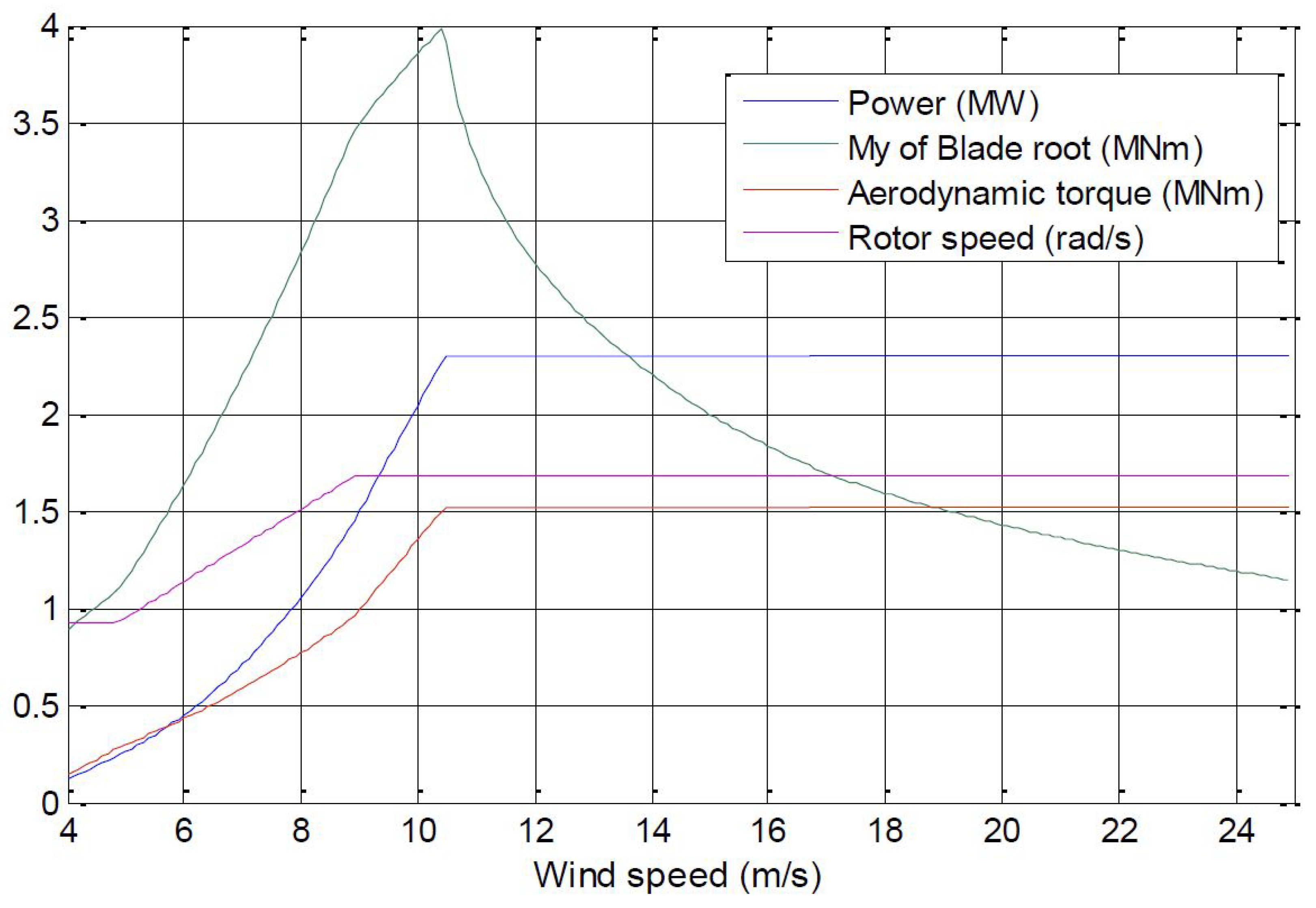
The steady state values for power, aerodynamic torque, rotor speed and flap-wise blade root bending moment are plotted against wind speed in Figure A1 [15]. The aeroelastic model of the wind turbine is constructed by downscaling a generic upwind, variable speed, pitch regulated 3 MW wind turbine model [23], using a similarity scaling rule [24,25,26]. The aerodynamic properties of the down-scaled model are adjusted according to the method reported in [27], where the aerodynamic properties of the blades were calculated by reverse engineering for the existing turbine.
Figure A1.
Variation of general parameters of wind turbine’s base model as a function of mean wind speed in steady-state conditions [15].
Figure A1.
Variation of general parameters of wind turbine’s base model as a function of mean wind speed in steady-state conditions [15].

The aeroelastic model of the turbine is validated against the data provided by the farm owner and used to obtain its operational loads of the existing wind turbine. This approach is common practice where the original aeroelastic model or measurement load data are not available [4]. The normal turbulence model (NTM) of IIB wind class with the corresponding 0.14 reference turbulence intensity and 0.2 wind shear coefficient is employed for normal power production, as recommended by the farm owner, based on the site’s wind properties. On this basis, the design load case DLC 1.2, which characterises the wind turbine loads over its power production range, connected to the grid, was applied as the reference design load over the turbine’s service life. The readers are referred to [15] for more information on the aeroelastic modelling and its validation.
Appendix B. Wind Rose Data
This paper investigates the lifetime extension source that stems from the variation of the mean wind speed direction over the turbine’s service life. For this purpose, a significant amount of wind rose data were deployed, which are subsequently presented in Appendices Appendix B.1 and Appendix B.2.
Appendix B.1. Case Study Wind Roses
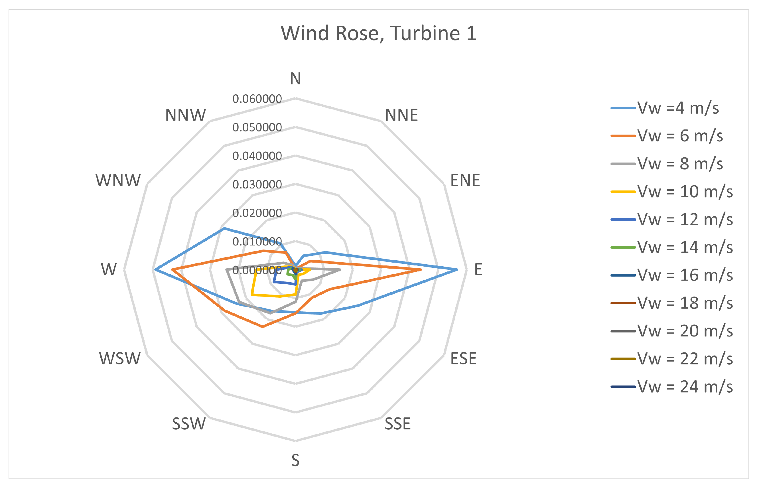
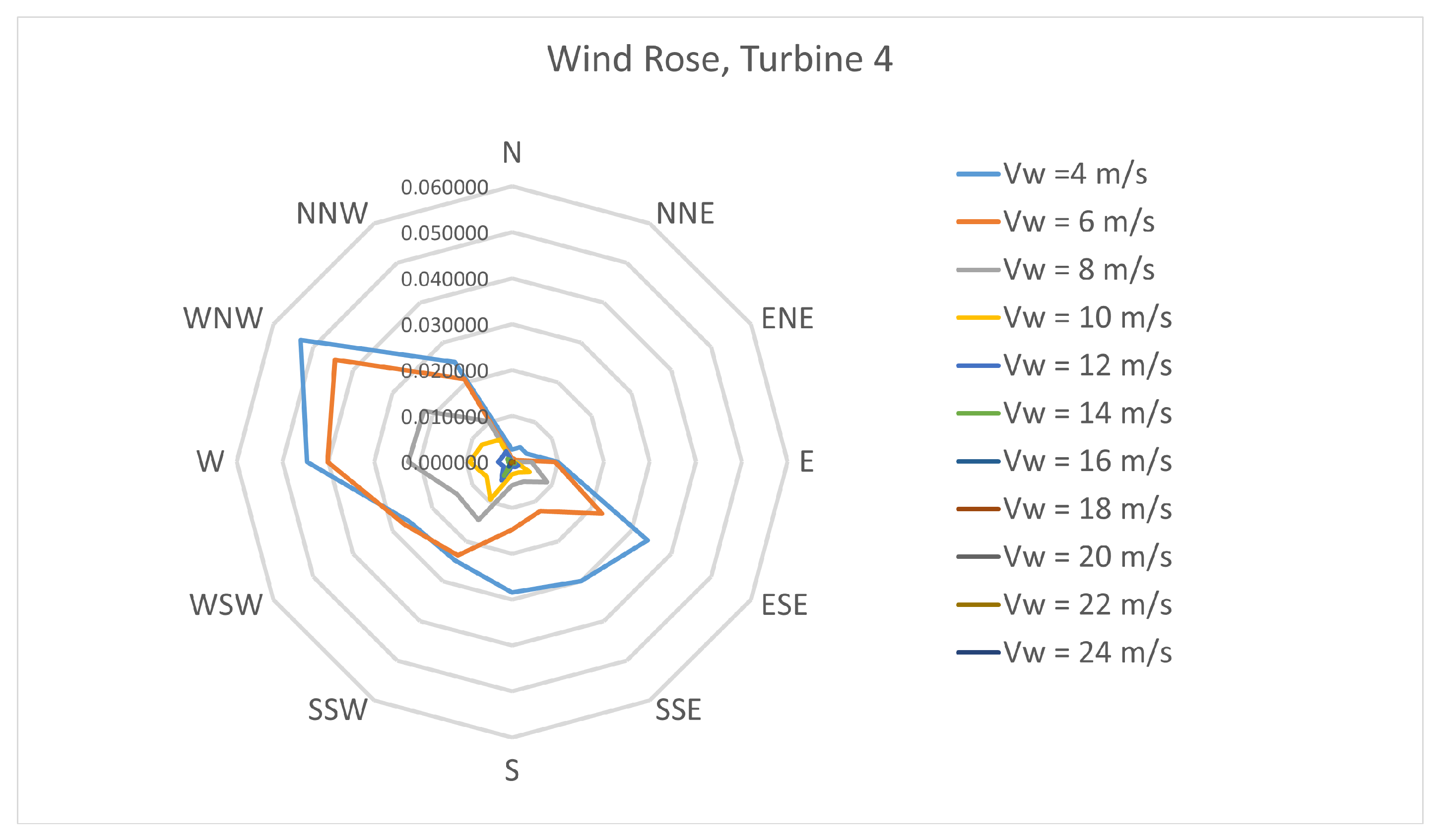
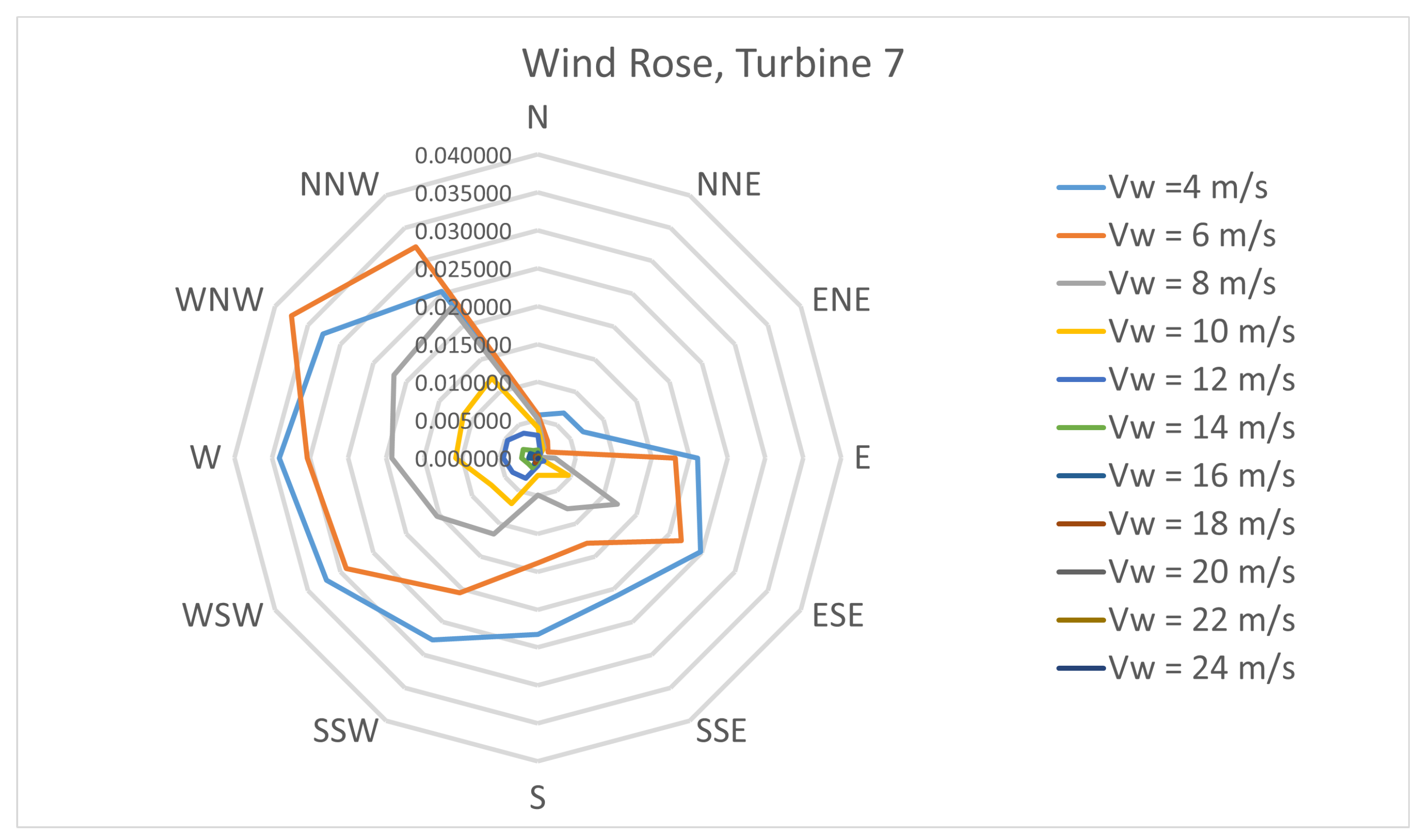
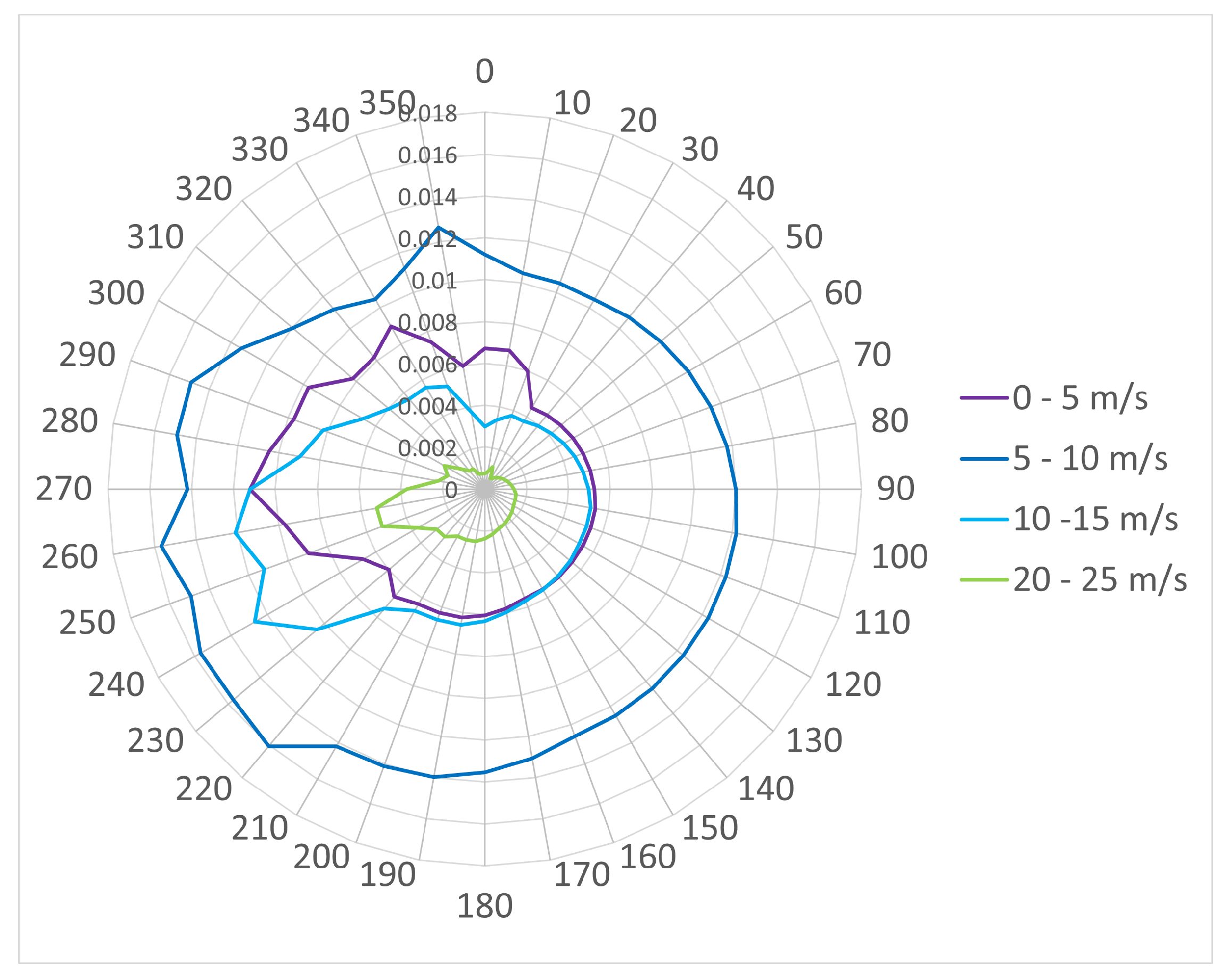
As discussed in Section 3.1 and Section 4.1, a series of wind roses were also required to carry out the analysis defined by the scenarios. SCADA data from seven wind turbines located on the case study wind farm are used for this paper. Three of these wind roses are shown in Figure A2, Figure A3 and Figure A4 as an example.
Figure A2.
Wind Rose 1—wind speed and wind direction probability for wind turbine 1 with prevailing wind direction.
Figure A2.
Wind Rose 1—wind speed and wind direction probability for wind turbine 1 with prevailing wind direction.

Figure A3.
Wind Rose 4—wind speed and wind direction probability for wind turbine 4.

Figure A4.
Wind Rose 7—wind speed and wind direction probability for wind turbine 7.

The wind roses provide the cumulative results of wind direction probabilities in bins of 30 and a range from 0 to 330 . In order to keep things straightforward, the same range and intervals are used for and in the closed-form solutions. Wind rose 1 (Figure A2) and 7 (Figure A4) were used for Scenario 1 within Section 3. The full range of wind roses were used for Section 4 both for Scenarios 1 and 2.
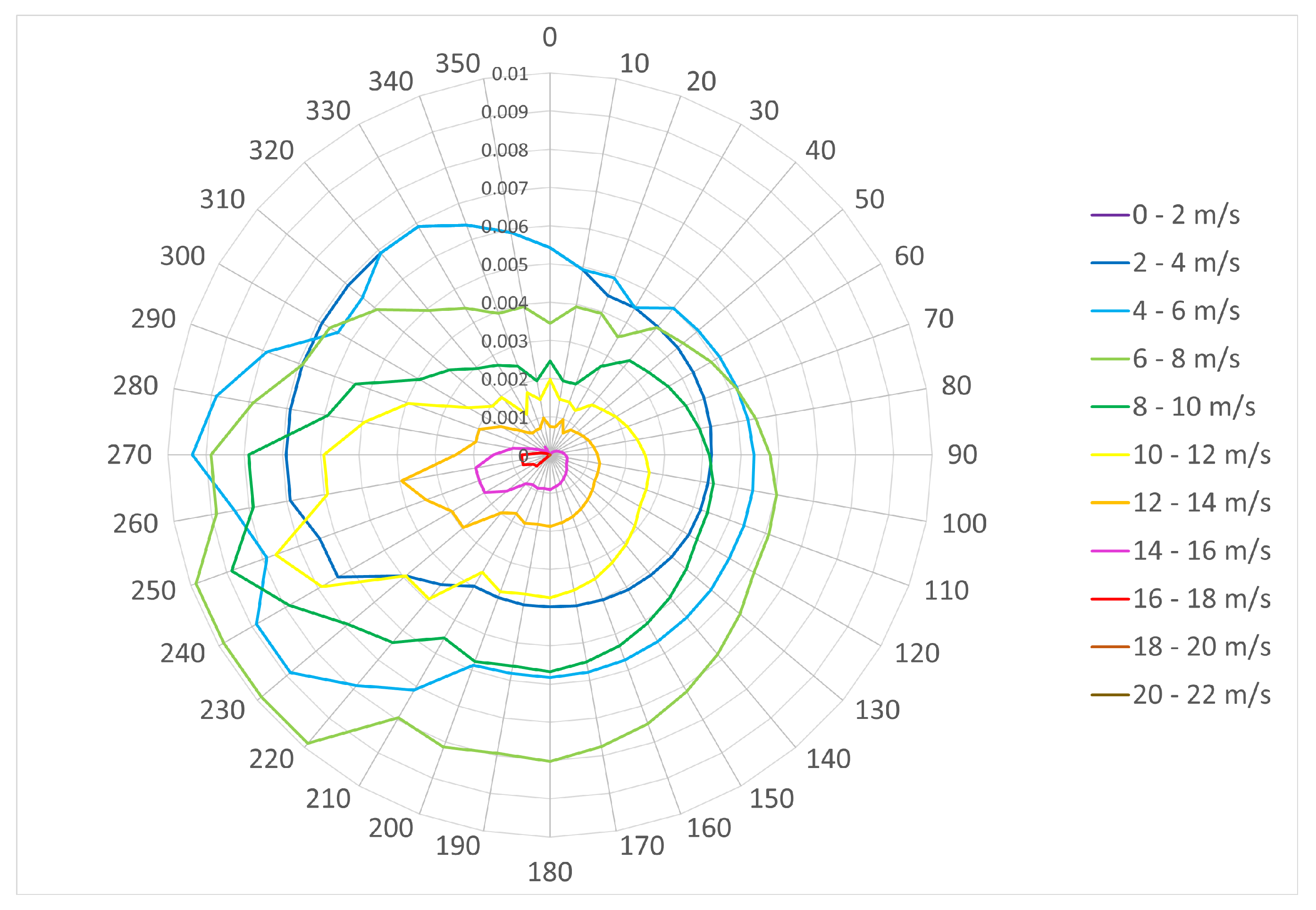
Appendix B.2. Additional Wind Roses
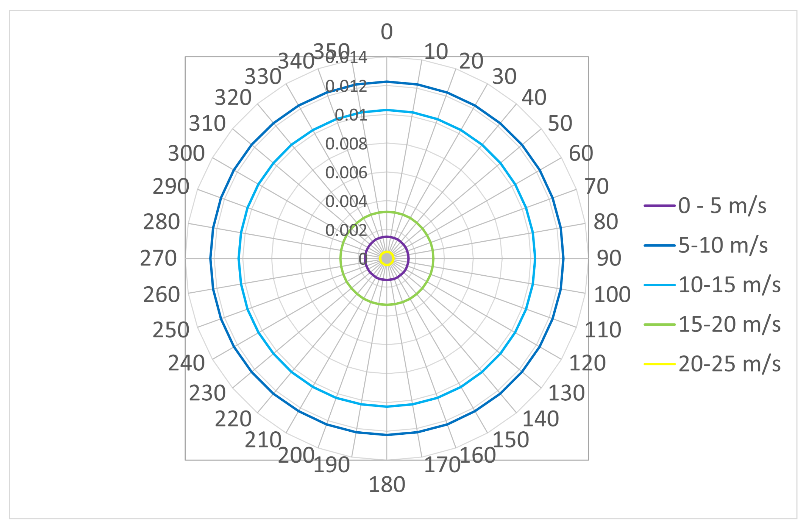
A second set of wind roses were used for Section 3 and Scenario 2. The first shown Figure A5 shows a hypothetical equally distributed wind rose. The second and third wind roses shown in Figure A6 and Figure A7 are extracted by the authors based on the actual but pictorial wind roses, in which the detailed data were not made available. Wind rose A and B have mean wind speed joint probabilities between 0 and 30 m/s within 5 m/s bins and mean wind direction joint probabilities between 0 and 360 in 10 bins. Wind rose C shows the mean wind direction joint probabilities between 0 and 360 in 10 bins, but the mean wind speed range is smaller (0 to 22 m/s) in 2 m/s bins according to the actual wind rose.
Figure A5.
Wind Rose A –An equally distributed wind rose.

Figure A6.
Wind Rose B – with prevailing wind direction.

Figure A7.
Wind Rose C – with prevailing wind direction.

References
- Ziegler, L.; Gonzalez, E.; Rubert, T.; Smolka, U.; Melero, J.J. Lifetime extension of onshore wind turbines: A review covering Germany, Spain, Denmark, and the UK. Renew. Sustain. Energy Rev. 2018, 82 Pt 1, 1261–1271. [Google Scholar] [CrossRef] [Green Version]
- Piel, J.H.; Stetter, C.; Heumann, M.; Westbomke, M.; Breitner, M.H. Lifetime Extension, Repowering or Decommissioning? Decision Support for Operators of Ageing Wind Turbines. J. Phys. Conf. Ser. 2019, 1222, 012033. [Google Scholar] [CrossRef]
- Bouty, C.; Schafhirt, S.; Ziegler, L.; Muskulus, M. Lifetime extension for large offshore wind farms: Is it enough to reassess fatigue for selected design positions? Energy Procedia 2017, 137, 523–530. [Google Scholar] [CrossRef]
- DNV, G.L. DNVGL-ST-0262 Lifetime Extension of Wind Turbines. Available online: https://rules.dnvgl.com/docs/pdf/DNVGL/ST/2016-03/DNVGL-ST-0262.pdf (accessed on 2 July 2019).
- Bureau Veritas. Move Forward with Confidence Guidelines for Wind Turbines Lifetime Extension. Technical Report 9, Bureau Veritas. 2017. Available online: https://www.bureauveritas.com/white-papers/Wind-turbines (accessed on 2 July 2019).
- Megavind. Report from Megavind: Useful Lifetime of a Wind Turbine. Technical Report, Megavind. 2016. Available online: https://megavind.winddenmark.dk/publications/strategy-extending-the-useful-lifetime-of-a-wind-turbine (accessed on 27 April 2022).
- Siemens Gamesa. Life Extension Service I Siemens Gamesa. Available online: https://www.siemensgamesa.com/products-and-services/service-wind/life-extension (accessed on 4 November 2019).
- Nabla Wind Power. Available online: http://www.nablawindpower.com (accessed on 10 January 2020).
- International Electrotechnical Commission. PT 61400-28 Wind Energy Generation Systems—Part 28: Through Life Management and Life Extension of Wind Power Assets. Available online: https://www.iec.ch/dyn/www/f?p=103:14:16178619540621::::FSP_ORG_ID:22048 (accessed on 1 September 2020).
- Ziegler, L.; Muskulus, M. Fatigue reassessment for lifetime extension of offshore wind monopile substructures. J. Phys. Conf. Ser. 2016, 9, 92010. [Google Scholar] [CrossRef]
- Tartt, K.; Nejad, A.; Kazemi Amiri, A.; McDonald, A. On Lifetime Extension of Wind Turbine Drivetrains. In Proceedings of the ASME 2021 40th International Conference on Ocean, OMAE2021, Online, 22–25 June 2021. [Google Scholar]
- International Electrotechnical Commission. IEC 61400-1 Wind Turbine -Part 1- Design Requirements. 2005. Available online: https://webstore.iec.ch/p-preview/info_iec61400-1%7Bed3.0%7Den.pdf (accessed on 1 September 2020).
- Rubert, T.; McMillan, D.; Niewczas, P. A decision support tool to assist with lifetime extension of wind turbines. Renew. Energy 2018, 120, 423–433. [Google Scholar] [CrossRef] [Green Version]
- Ziegler, L.; Cosack, N.; Kolios, A.; Muskulus, M. Structural monitoring for lifetime extension of offshore wind monopiles: Verification of strain-based load extrapolation algorithm. Mar. Struct. 2019, 66, 154–163. [Google Scholar] [CrossRef]
- Amiri, A.K.; Kazacoks, R.; Mcmillan, D.; Feuchtwang, J.; Leithead, W. Farm-wide assessment of wind turbine lifetime extension using detailed tower model and actual operational history. J. Phys. Conf. Ser. 2019, 1222, 012034. [Google Scholar] [CrossRef]
- Natarajan, A.; Pedersen, T.F. Remaining Life Assessment of Offshore Wind Turbines Subject to Curtailment. In Proceedings of the International Offshore and Polar Engineering Conference, Sapporo, Japan, 10–15 June 2018; pp. 527–532. [Google Scholar]
- Slot, R.M.M.; Schwarte, J.; Svenningsen, L.; Sørensen, J.D.; Thøgersen, M.L. Directional Fatigue Accumulation in wind turbine steel towers. J. Phys. Conf. Ser. 2018, 1102, 012017. [Google Scholar] [CrossRef]
- DNV-GL. Bladed, Wind Turbine Design Software, Version 4.8; DNV-GL: Bærum, Norway, 2016. [Google Scholar]
- International Electrotechnical Commission. IEC 61400-13 Wind Turbine Part 13: Measurement of Mechanical Loads. Technical Report, IEC. 2016. Available online: webstore.iec.ch/publication/23971 (accessed on 1 September 2019).
- Veers, P.S. Chapter 5 Fatigue Loading of wind turbines. In Wind Energy Systems: Optimising Design and Construction for Safe and Reliable Operation; Woodhead Publishing Ltd.: Sawston, UK, 2010; pp. 130–158. ISBN 978-18-4569580-4. [Google Scholar] [CrossRef]
- Dowling, N.E. Mechanical Behaviour of Materials; Pearson Education Ltd.: London, UK, 2013; ISBN 978-01-31395-06-0. [Google Scholar]
- Lee, Y.; Pow, J.; Hathaway, R.; Barkey, M. Fatigue Testing and Analysis, Theory and Practice; Butterworth-Heinemann: Oxford, UK, 2004; ISBN 978-0-7506-7719-6. [Google Scholar]
- Kazacoks, R. A Generic Evaluation of Loads in Horizontal Axis Wind Turbines. Ph.D. Thesis, University of Strathclyde, Glasgow, UK, 2017. [Google Scholar]
- Ashuri, T. Beyond Classical Upscaling: Integrated Aeroservoelastic Design and Optimization of Large Offshore Wind Turbines; Wohrman Print Service: Zupthen, The Netherlands, 2012; ISBN 978-94-6203-210-1. [Google Scholar]
- Manwell, J.; McGowan, J.; Rogers, A. Wind Energy Explained; John Wiley & Sons, Ltd.: Chichester, UK, 2002; p. vii 577. [Google Scholar]
- Jamieson, P. Innovation in Wind Turbine Design; John Wiley & Sons, Ltd.: Chichester, UK, 2011; p. 298. ISBN 047-06-99817. [Google Scholar]
- Carlen, I. Aerodynamic Characteristics for the Siemens-2.3-93 Rotor; Technical Report; Siemens: Berlin, Germany, 2012. [Google Scholar]
Figure 1.
Flowchart of lifetime extension potential assessment [15].
Figure 1.
Flowchart of lifetime extension potential assessment [15].

Figure 2.
Wind turbine elevation co-ordinate system [18] (left), the tower co-ordinate system and cross section parameters as defined in this study (right).
Figure 2.
Wind turbine elevation co-ordinate system [18] (left), the tower co-ordinate system and cross section parameters as defined in this study (right).

Figure 3.
Aeroelastic model results for wind speed for a below-rated wind speed of 6 m/s.

Figure 4.
Aeroelastic model results for wind speed for a rated wind speed of 10 m/s.

Figure 5.
Aeroelastic model results for wind speed for an above-rated wind speed of 22 m/s.

Figure 6.
Aeroelastic model results for fluctuating angle between hub thrust and lateral forces for wind speed for a below-rated wind speed of 6 m/s.
Figure 6.
Aeroelastic model results for fluctuating angle between hub thrust and lateral forces for wind speed for a below-rated wind speed of 6 m/s.

Figure 7.
Aeroelastic model results for fluctuating angle between hub thrust and lateral forces for wind speed for a rated wind speed of 10 m/s.
Figure 7.
Aeroelastic model results for fluctuating angle between hub thrust and lateral forces for wind speed for a rated wind speed of 10 m/s.

Figure 8.
Aeroelastic model results for fluctuating angle between hub thrust and lateral forces for an above-rated wind speed of 22 m/s.
Figure 8.
Aeroelastic model results for fluctuating angle between hub thrust and lateral forces for an above-rated wind speed of 22 m/s.

Figure 9.
Deviation for below-rated wind speed (6 m/s).

Figure 10.
Deviation for rated wind speed (10 m/s).

Figure 11.
Deviation for above-rated wind speed (22 m/s).

Figure 12.
Cos term evaluation for a below-rated wind speed (6 m/s) for set , (above) and for set , (below).
Figure 12.
Cos term evaluation for a below-rated wind speed (6 m/s) for set , (above) and for set , (below).

Figure 13.
Cos term evaluation for rated wind speed (10 m/s) for set , (above) and for set , (below).
Figure 13.
Cos term evaluation for rated wind speed (10 m/s) for set , (above) and for set , (below).

Figure 14.
Cos term evaluation for above-rated wind speed (22 m/s) for set with , (above) and for set with , (below).
Figure 14.
Cos term evaluation for above-rated wind speed (22 m/s) for set with , (above) and for set with , (below).

Figure 15.
Histograms of 10 min bending stress , resultant bending moment M, and fore-aft bending moment time series for below-rated mean wind speed (6 m/s), set , (above), set (below).
Figure 15.
Histograms of 10 min bending stress , resultant bending moment M, and fore-aft bending moment time series for below-rated mean wind speed (6 m/s), set , (above), set (below).

Figure 16.
Histograms of 10 min bending stress , resultant bending moment M, and fore-aft bending moment time series for rated mean wind speed (10 m/s), set , (above), set (below).
Figure 16.
Histograms of 10 min bending stress , resultant bending moment M, and fore-aft bending moment time series for rated mean wind speed (10 m/s), set , (above), set (below).

Figure 17.
Histograms of 10 min bending stress , resultant bending moment M, and fore-aft bending moment time series for above-rated mean wind speed (22 m/s) set , (above), set (below).
Figure 17.
Histograms of 10 min bending stress , resultant bending moment M, and fore-aft bending moment time series for above-rated mean wind speed (22 m/s) set , (above), set (below).

Figure 18.
Normalised damage equivalent load associated with uni-directional fatigue damage using 10 min bending stress , resultant bending moment M and fore-aft bending moment time series where and are fixed at 0 (above) and where and are fixed at 60 and 30 , respectively (below).
Figure 18.
Normalised damage equivalent load associated with uni-directional fatigue damage using 10 min bending stress , resultant bending moment M and fore-aft bending moment time series where and are fixed at 0 (above) and where and are fixed at 60 and 30 , respectively (below).

Figure 19.
Comparison of normalised damage equivalent load associated with uni-directional fatigue damage using 10 min bending stress time series with and without Goodman’s correction where and are fixed at 0 .
Figure 19.
Comparison of normalised damage equivalent load associated with uni-directional fatigue damage using 10 min bending stress time series with and without Goodman’s correction where and are fixed at 0 .

Figure 20.
Absolute between uni-directional fatigue damage and fatigue damage at a range of tower positions for wind rose 1.
Figure 20.
Absolute between uni-directional fatigue damage and fatigue damage at a range of tower positions for wind rose 1.

Figure 21.
Absolute between uni-directional fatigue damage and fatigue damage at a range of tower positions for wind rose 1 with the application of the Goodman’s correction factor.
Figure 21.
Absolute between uni-directional fatigue damage and fatigue damage at a range of tower positions for wind rose 1 with the application of the Goodman’s correction factor.

Figure 22.
Absolute between uni-directional fatigue damage and fatigue damage at a range of tower positions for a range of wind roses.
Figure 22.
Absolute between uni-directional fatigue damage and fatigue damage at a range of tower positions for a range of wind roses.

Figure 23.
Normalised calculated using bending stress , resultant bending moment M and fore-aft bending moment for a range of wind turbines.
Figure 23.
Normalised calculated using bending stress , resultant bending moment M and fore-aft bending moment for a range of wind turbines.

Figure 24.
Percentage difference in normalised between resultant bending moment M and fore-aft bending moment and bending stress , for a range of wind turbines.
Figure 24.
Percentage difference in normalised between resultant bending moment M and fore-aft bending moment and bending stress , for a range of wind turbines.

Figure 25.
Normalised using bending stress with and without the application of the Goodman’s correction factor for a range of wind turbines.
Figure 25.
Normalised using bending stress with and without the application of the Goodman’s correction factor for a range of wind turbines.

Figure 26.
Normalised using wind rose data only for a range of wind turbines.

Figure 27.
Normalised results for a range of scenarios compared to relative calculated using finite element analysis for a range of wind turbines.
Figure 27.
Normalised results for a range of scenarios compared to relative calculated using finite element analysis for a range of wind turbines.

Figure 28.
Relative lifetime extension potential for a range of scenarios range of wind turbines.

Table 1.
Farm-wide overview of lifetime potential for case study wind turbines 1 to 6 relative to turbine 7.
Table 1.
Farm-wide overview of lifetime potential for case study wind turbines 1 to 6 relative to turbine 7.
| Lifetime Extension Potential | ||||||
|---|---|---|---|---|---|---|
| Wind Turbine | Bending Stress | Bending Stress with Goodman’s | Resultant Bending Moment M | Fore-Aft Bending Moment | Wind Rose only | FEA |
| Scenario 1, estimate (i) | Scenario 1, estimate (i) | Scenario 1, estimate (ii) | Scenario 1, estimate (iii) | Scenario 2, estimate (iv) | Independent analysis | |
| 1 | 0.800 | 0.708 | 0.882 | 0.875 | 0.659 | 0.757 |
| 2 | 0.477 | 0.424 | 0.543 | 0.537 | 0.549 | 0.536 |
| 3 | 0.861 | 0.856 | 0.924 | 0.917 | 0.836 | 0.883 |
| 4 | 1.455 | 1.430 | 1.540 | 1.532 | 1.275 | 1.491 |
| 5 | 1.420 | 1.404 | 1.500 | 1.493 | 1.212 | 1.449 |
| 6 | 0.928 | 0.856 | 1.020 | 1.014 | 0.816 | 0.923 |
Publisher’s Note: MDPI stays neutral with regard to jurisdictional claims in published maps and institutional affiliations. |
© 2022 by the authors. Licensee MDPI, Basel, Switzerland. This article is an open access article distributed under the terms and conditions of the Creative Commons Attribution (CC BY) license (https://creativecommons.org/licenses/by/4.0/).
Share and Cite
MDPI and ACS Style
Grieve, N.; Kazemi Amiri, A.M.; Leithead, W.E. A Straightforward Approach to Site-Wide Assessment of Wind Turbine Tower Lifetime Extension Potential. Energies 2022, 15, 3380. https://doi.org/10.3390/en15093380
AMA Style
Grieve N, Kazemi Amiri AM, Leithead WE. A Straightforward Approach to Site-Wide Assessment of Wind Turbine Tower Lifetime Extension Potential. Energies. 2022; 15(9):3380. https://doi.org/10.3390/en15093380
Chicago/Turabian StyleGrieve, Nicola, Abbas Mehrad Kazemi Amiri, and William E. Leithead. 2022. "A Straightforward Approach to Site-Wide Assessment of Wind Turbine Tower Lifetime Extension Potential" Energies 15, no. 9: 3380. https://doi.org/10.3390/en15093380
Note that from the first issue of 2016, this journal uses article numbers instead of page numbers. See further details here.