Abstract
The paper aims to propose a method of reconfiguring the train timetable, taking into account minimising the globally consumed energy for traction purposes. This is a very important issue in the context of rising electricity prices, alarming climate changes and the “Fit for 55” policy introduced in Europe. Each unit of energy saved contributes to improving the state of the planet and reducing the negative human impact on it. In this paper, the authors propose a model that, when applied, will reconfigure the timetable in terms of energy intensity and, as a result, reduce the impact of railways on the burden on the environment. It is proposed to introduce an interdependence between trajectories of electrical train movement. This interdependence is to take place so that it is possible to efficiently transfer the energy recovered during the braking of one train to another train, moving on the same section of the railway line and at the same time (i.e., without using energy storage devices). The paper provides a physical background to the considerations—discussing the movement of electric trains in the context of their energy intensity and the possibility of energy recovery; presenting the possibility of interconnecting trains in such a way that the energy from a train that is being braked can be efficiently used by a train that is being accelerated; presenting a method for making the linkages between trains (in the form of an original algorithm resulting from the application of the Delphi method) and implementing them in the timetable. The timetable for the application of the method is real and was obtained from the railway operator in Poland, as a mathematical–physical model describing the trajectory and energy consumption of the original, after which the proposed timetable was verified by running simulations and comparing the energy consumption of the original and the proposed timetable. It turned out that it is possible to achieve a global total energy demand reduction of up to 398 MWh/year. This proves the validity of using the proposed algorithm at the timetabling stage and extending its implementation to the entire network. Furthermore the authors also recognise the tendency of the algorithm to return repeatable solutions, which has the side effect of creating a cyclic timetable. Its implementation in Poland has proved impossible for many years. The application of the proposed method could change this unfavourable situation.
1. Introduction
Rail, especially electric rail, is one of the most environmentally friendly means of transport [1]. It has a low energy intensity per passenger or tonne of freight. It leaves a relatively small carbon footprint. Carbon dioxide emissions are several times lower for rail than for other modes of transport. As a result, rail is promoted by numerous international organisations (including the European Union) as environmentally friendly and part of sustainable development or green mobility policies. The European Union plans to reduce greenhouse gas emissions produced from transport by at least 60% by 2050 in relation to the reference year (1990) [2]. This is part of the “Fit for 55” policy. These characteristics mean that the use of rail for the transport of goods and services is growing and is expected to continue to grow [3]. Any initiative leading to a reduction in the negative impact of human activity on the cleanliness of the planet and its ecosystem is very important in this context. The conscious choice of rail as a mode of transport in itself contributes to improving the state of the environment. However, implementing initiatives to make railways ever more environmentally friendly will further improve the balance of benefits of using electric trains.
Through the economies of scale of such relatively small initiatives in the context of the country as a whole, it is possible to reduce electricity demand to such an extent that it may become unnecessary to maintain, for example, a coal-fired power plant. The closure of such a facility will, by definition, improve the country’s energy mix by reducing the share of conventional energy sources in favour of increasing the share of non- and low-carbon sources.
Moreover, rail can be an important political tool. Sovereign states are often independent in terms of electricity from their neighbours (or work within a closely interconnected system, covering the territory of at least several states—e.g., as in the EU), and can generate it on their own, for their use. However, the use of other sources of power—for example, coal, gas or liquid and gaseous fuels—often entails the need to sign unfavourable agreements with countries from which—for political reasons—one should not cooperate. Reducing the energy intensity of railways may therefore also influence the independence of states by reducing fuel imports from third countries.
Unfortunately, the energy crisis that the world is increasingly struggling with, that has increased fuel prices, is also affecting railways. In this context, it seems reasonable to further reduce the energy intensity of this branch of transport. Additionally, the policy pursued in the context of reducing pollutant emissions necessitates an increase in the energy efficiency of the railway system [4]. Reducing the global energy requirements of railways can be achieved, for example, by making better use of the energy that can be recovered from braked vehicles [5,6,7]. The potential for such action appears to be very significant.
In 2019, passenger trains stopped at stops and railway stations more than 29.3 million times in Poland [8]. This does not include reducing velocity before limits, technical stops, train brakes performed as part of a dynamic brake test, train brakes during service journeys, brakes performed during shunting journeys, brakes due to stops not provided for in the timetable but caused by the traffic situation, and stops and speed reductions of goods trains. In practice, this could mean several hundred million train breaks occurred in just one country. Instead, this energy can be used to power trains at speed or a constant speed. The direct transfer of electrical energy from a braked train to an accelerating train can be achieved without significant interference with the power supply system, provided that the recovered energy is immediately used by another vehicle. It is provided that the recovered energy is immediately used by another vehicle [9,10]. Otherwise, it is necessary to convert DC substations (found in some European countries) to reversible substations that facilitates current flow in both directions. Otherwise, it is required to convert DC substations (DC is using in some European countries) to reversible substations that allow for a current flow in both directions as long as the trains are running within the same supply section. One section usually comprises several kilometres of railway (from 7 to 20 km in the DC power supply [11]), and several trains generally travel within this section.
Because of the facts presented, the issue of reducing the global electricity demand of the railway system is fundamental. However, it is possible to achieve this by transferring the braking energy from one train to other trains while they are accelerating in the same supply section. Such a section is long enough for several trains to run at the same time. Moreover, this approach does not require initiatives to convert hundreds or, in the case of some countries, thousands of kilometers of overhead contact lines and substations along the line. However, it should be borne in mind that the efficiency of such a process is limited and depends, among other things, on the configuration of the trains. The configuration of trains is a direct consequence of the timetable, which determines the occurrence times of the phases of movement for each train. Therefore, to increase the possibility of using the braking energy of one train for the acceleration of other trains, it makes sense to develop a method for reconfiguring the timetable in such a way as to make maximum use of the potentially available energy.
This article proposes a method for reducing the global energy intensity of railways by reconfiguring train schedules. The method’s application consists of postponing some trains or changing the mode of acceleration or braking (by staging the process). It takes into account the available capacity of railway lines.
The proposed method can be defined as an algorithm, which is applied at the stage of preparing the train timetable, after the preliminary arrangement of routes (determined by railway undertakings) and journey hours (based on railway line characteristics and parameters of the trainsets running on it).
The timetable is prepared by the railway line manager based on so-called traction calculations, also quoted in this article. They are made with the use of formulas determined empirically by national institutes engaged with railway research. Such formulae—obtained from the national railway institutes of the countries associated with the UIC (International Union of Railways). have also been converted to an individualised form for each train.
The proposed method was developed using the Delphi method. The method was verified by determining traffic trajectories of particular trains based on the existing and valid timetable announced by the Polish rail infrastructure manager—PKP PLK SA and technical information on train parameters (data from the rolling stock manufacturers). This was performed for one of the railway lines leading from Wrocław (Poland). Then, for the trajectory of train traffic developed in this way and after determining the energy consumption caused by their movement, the proposed method was applied. The results for the unchanged and the changed timetable were then compared with each other. In this way, it was possible to estimate the value of the change in energy intensity. Importantly, this paper discusses the results of applying reconfiguration to only weekday timetables. Due to the similarity of the issue, a detailed presentation of the reconfiguration results for Saturdays and Sundays is not presented. However, these values were included in the final estimation.
The article is structured as follows. Section 2 discusses the views already proposed on the problem of using recovered energy for train acceleration and shows the gap that the proposed method fills. Section 3 discusses the method, including its soundness from a physics point of view and introduces and describes the algorithm. Section 4 discusses the results of the proposed method based on a comparison of the energy consumption results of the non-reconfigured and the reconfigured timetable. The conclusion is given in Section 5.
2. Literature Review
The problem of reducing the energy intensity of the railway system has been recognised in works published so far. The authors have proposed various solutions, looking at reducing the energy demand of electric trains from multiple aspects. The authors propose three basic approaches, including reconstruction of railway lines power supply system (in case of solutions using direct current), optimisation of the trajectory of single train movement, and reconfiguration of timetable.
An in-depth literature review on increasing the energy efficiency of the railway system is presented in the paper [12]. The authors collected 123 literature references regarding ways and methods of energy-efficient railway operation in the case of DC power supply. Additionally, in their work [13], Lin et al. detail dozens of methods for the energy optimisation of train movement, focusing, however, on the possibilities of modifying vehicle trajectories and the applied driving phases.
In terms of power-system modification, one of the solutions to reduce energy consumption is the replacement of the classical DC electric substation with a reversible substation [10]. The authors highlights that this presents the possibility of recovering electrical energy without reconfiguring the timetable, so they do not consider this aspect worth applying. At the same time, they recognise that a timeline that has not been drawn up with energy efficiency in mind—despite its strong traffic determinism—introduces de facto randomness in train stops globally. Petru et al. [14] proposed the use of supercapacitors in metro trains. Arboleya et al. [15] proposed a train that included an onboard hybrid accumulation system used in DC traction networks. In ref. [16], the optimisation of the speed profile during train running was combined with energy storage installation inside the vehicle. In ref. [17], it was reported that it is possible to return electricity to the grid or store it in energy storage tanks (ESS). A hybrid approach is presented in ref. [18]. It is linked to electricity recovery and speed profile optimisation. However, the study only applies to metropolitan railways, which are usually homogeneous (due to the vehicles used).
The metho of reducing the energy intensity of rail transport by optimising the movement of individual trains and improving their trajectories has also been recognised in several works. This is a classic technique that has been used on various railways for several decades. However, the methods are various, but generally—at an earlier or later stage—they come down to a common denominator. In ref. [19], the coasting technique is proposed to improve energy savings in railways. The authors transferred the train control problem into a multi-step decision problem and they introduced the Dynamic Programming method to calculate the energy-efficient driving strategy with the given trip time. Next, they optimised trip times and the headway of trains using the Simulated Annealing algorithm based on the results of the dynamic programming method. The installation of a hardware and software system onboard the train to supervise the electric locomotive’s operation and maximise the runaway time has also been proposed. Another proposal in the field of trajectory modification is provided in ref. [20], which proposes using computer microsimulation (OpenTrack tool) to optimise the trajectory of one train to minimise energy demand. In refs. [21,22], the authors propose the application of the Ant Colony Algorithm to the train scheduling optimization problem. Ref. [21] develops a new algorithm for the train scheduling problem using Ant Colony System (ACS) meta-heuristic, while ref. [22] describes an Ant Colony Optimization (ACO) algorithm for the train routing selection problem (TRSP). A classical approach is represented by ref. [23], which pays attention to the possibility of controlling the energy demand of a train by changing the driving modes. In ref. [24], the authors propose the management of the trajectory of a freight train moving over long sections with a uniform gradient. They note that coasting does not, in all conditions, imply the least energy-intensive option. A classical approach is also proposed in ref. [25]. The authors propose a Simulated Annealing optimisation algorithm that minimises train traction energy, constrained to the existing timetable. A classical approach for modifying motion trajectories is also presented in ref. [26]. However, the authors implement the modification of train movement phases into an autonomous train operation (ATO) system. They improved the multi-objective hybrid optimisation algorithm using a comprehensive learning strategy (ICLHOA).
The literature also recognises the possibility of reducing the energy intensity consumption of railways by making the movement of several vehicles dependent on each other and transferring the energy recovered from breaking one train to another vehicle. Such an approach is presented, among others, in ref. [27], where Bu et al. discuss the use of electric energy recovered from a braking vehicle to an accelerating vehicle with the example of an urban railway network, i.e., with fixed intervals and very homogeneous traffic. A similar approach was proposed in [28]. They proposed the synchronisation of metro train schedules. A particular nuance here is the consideration of two types of moving vehicles. However, the problems related to the occurrence of fixed intervals are characteristic of the cases described in this paper. Pairing trains moving in opposite directions over long sections with a uniform gradient and transferring energy between them was proposed in ref. [29] where authors noticed that a train moving down a hill must be continuously braked to avoid over-speeding.
In contrast, a train moving “uphill” must overcome the additional resistance of the hill. Therefore, they proposed that the braking energy of the descending train should be continuously recovered and used by the accelerating train to overcome the resistance of the hill. This approach—shifting trains in time—is interesting, but the problem is somewhat when implementing a regular railway system. A slightly different strategy is described by Gong et al. [30], as they propose modifying the timetable by extending train stops at stations, which is supposed to synchronise accelerations and decelerations. This, in turn, is supposed to allow the braking energy to be used for the start-up of another train. Peña-Alcaraz et al. [31] also proposed controlling the overlap between the running phases of different trains. However, his approach differs from the work of ref. [20] by preferring the modification of arrival and departure times and not only the control of stopping times. In the context of managing energy links between several trains, interesting thoughts are brought by the work of Bu et al. [32]. The researchers developed a model for designing an energy-efficient timetable that considers the links between adjacent trains under acceleration and deceleration. The global energy efficiency of the system is supposed to be ensured by permissibly varying the speed of the coordinated trains. However, this approach can significantly impact journey times, and therefore rail-line capacity may be reduced.
The following table (Table 1) provides a summary of the articles discussed along with information on the area of rationalisation (optimisation) to minimise the energy intensity of railways by modifying the timetable.

Table 1.
Methods of optimising train schedules to reduce energy intensity.
A review of the state of knowledge confirms the authors’ conviction that the problem of reducing the energy consumption of rail transport is important and topical. Many researchers have looked into this issue and made suggestions on how to make railways even more energy-efficient. There are many views and ideas for action. Some of them concern modifications to the power supply system (changes are necessary in DC power supply systems), others have investigated the possibility of building in devices that could temporarily store excess electrical energy. Concepts are also based on the idea of modifying the trajectory of trains to generate interdependencies between the accelerating train and the braking train. However, these approaches usually concern homogeneous systems (metro, light rail—due to the rolling stock used, long stretches of homogeneous gradient freight line—due to the very long cooperation time of two trains). There are relatively few proposals for methods that take mixed traffic railway lines into account.
3. Methodology
The following section discusses the methodology of the global electricity demand reduction method. In Section 3.1, the physical aspect of recovering electricity and using it for traction purposes (propelling) of another train is presented. Section 3.2 presents and discusses the algorithm that constitutes the method.
The application of the method should be preceded with an analysis of the existing timetable and the determination for it (using the empirical formulae discussed in Section 3.1 of this paper) of the current capacity of the electrical substation as a function of time. This may be a pre-arranged timetable under development, but it may also be, as in the case discussed in this article, a timetable already in force. The next step is to implement the presented reconfiguration algorithm into the base timetable (described in Section 3.2). This will move the trains in relation to a certain time interval to obtain a better energy-efficient timetable. The third step is to perform an analysis of the current capacity for the modified variant. Finally, the energy-consumption status of the timetable for the primary and secondary variants should be compared. The methodology adopted for the application of the proposed algorithm makes it possible to determine the synthetic value of the electricity that can be saved.
3.1. Electricity Demand of the Train
The characteristics of the driving parameters of a railway vehicle can be obtained by solving the equation of the motion of a train [33,34,35,36,37]. The equation of the motion of a train is based on Newton’s second law of dynamics. A second-order differential equation describes it:
where F is the resultant force (depend on velocity v and displacement x), m the mass, k the coefficient of swirling mass, time (t). The resultant force depends on tractive effort (Z), resistance effort of train movement (W), braking force (B) and resistance resulting from the route of the railway line (I). These forces—depending on the driving mode—occur in different configurations. Forces: tractive (Z) resistance (W) and braking (B) also depends on the velocity of the moving train (v). Resistance resulting from the route of the railway line depends on displacement. These forces shall be applied depending on the train mode [31,32,33,34].
The current (In) drawn from the overhead line by the electric train is proportional to the power (P) and inversely proportional to the voltage (U):
The magnitude of current consumption recorded in an electrical substation is higher than that derived from the solved equation of train movement. This is due to current transmission losses and the inefficiency of technical equipment, especially traction motors, and other consumers of energy on the train, i.e., air conditioning, heating, lighting, passenger information systems, brake compressor drive, propulsion control system, etc. It is, therefore, necessary to account for these factors when determining the actual load on an electrical substation (Ient). For this purpose, the value specified by Equation (2) has to be corrected:
where η1 is the efficiency of contact line (0.91); η2 is the efficiency, counting aberrant movement work (0.98); η3 is the efficiency of the electricity substation (0.94) [33,35]. is the current drawn by other consumers, such as lighting, air conditioning, heating, passenger information system and connected passengers’ devices. The values given above are averages taken globally for the entire electric traction at 3 kV DC. Railway administrations adopt—from experience—values similar to those shown above. In practice, electric traction efficiency values are provided in ranges of a few per cent [33].
We also know that:
where F means acceleration force.
The formula can define the work (W) performed by the i-th train:
After the transformation of Equations (3) and (5) and subrogation of Equations (1) and (4), the formula for i-th train work can be obtained:
In order to reduce the energy demand of the whole railway system, the total energy intensity (TEI) of the trains running on a given section of line will be verified:
Reducing the railway system’s total energy demand may involve transferring the energy recovered during vehicle braking to another train. In this case, it is necessary to consider the efficiency of the system for recovering braked energy and the efficiency of transferring this energy to another train. This approach is more convenient than using the value of the current flowing from the train being braked to the accelerating train or the power that can be transferred between the previously mentioned trains. The method for minimising energy demand for all trains on a railway line is described in detail in Section 3.2.
The amount of current drawn by a train and the momentary ability to transfer energy to another vehicle is determined by the driving mode the train is in.
The train may be accelerating, it may be moving at a constant speed, it may be running with the traction motors switched off (coasting), or it may be braking. In the acceleration mode, the driving force Z(v) at the wheels of the train has to overcome the values of resistance to motion W(v) and resistance to climb I(x). Such a train will draw its electrical energy from the overhead contact line.
A train moving at a constant speed must balance the value of the resistance acting on it; therefore, the value of the acceleration force must be equal to 0. Such a train can be both accelerated and braked (when the values of the locomotive resistances are negative and overcome the importance of the specific resistances). The train can run in coast-down mode. Then, the electric motors are switched off and the resultant acceleration force F(v,x) depends only on the resistance. The last mode is the braking mode, where the train speed is reduced due to braking. In this mode, energy recovery is possible. The driving modes are presented graphically in Figure 1.
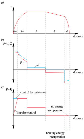
Figure 1.
Four train-running modes: 1a—starting (according to the constant acceleration curve), 1b—acceleration (according to the course of the hyperbola of continuous power), 2—running at a constant speed, 3—running from coasting, 4—braking. (a) Velocity versus distance graph; (b) acceleration and acceleration force (red line) and tractive effort (blue line) versus distance graph; and (c) power and energy of running train with impulse (red on first movement phase) and resistance (blue) control or (in phase 4) braking energy with recuperation (green) and without recovery (red).
According to research, it is possible to transfer around 70% of braking energy to another train. The highest values obtained fluctuated around 73% [17].
The abovementioned factors provide an idea of the possible actions that can be taken in modifying the trajectory of one train in order to couple it with that of another. It is possible to control the movement trajectory in such a way related not only to the phases of movement, i.e., so that the acceleration of one train and braking of the other train coincide, but it is also possible, for example, to introduce a phase of running at a constant speed between two stages of acceleration. It is relatively plausible to break a train in several steps. Table 2 lists the possible actions for interdependent train paths depending on the need to use the contagious energy.
Table 2.
List of possible measures within the framework of a reconfiguration of the timetable, taking into account increased energy efficiency of the railways.
Figure 2 gives an idea of how trains can depend on each other to reduce energy intensity.
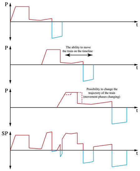
Figure 2.
The gist of the issue.
The top three figures show the power consumption of different trains as a function of time. The bottom figure is the sum of these values. The situation is presented as it was, without considering the application of the method. In addition, the central figures graphically present how changes in train trajectories will be implemented.
3.2. The Algorithm
The developed algorithm considers the limitations that exist in the given supply section (e.g., speed limits, track infrastructure and traffic routing) and the rules resulting from the timetable assumptions in the area of the commercial offer. This means that it is possible to change the timetable, but the individual departure times from individual stations must be within the specified time intervals defined in the commercial offer. The operation of the algorithm is presented in Figure 3.
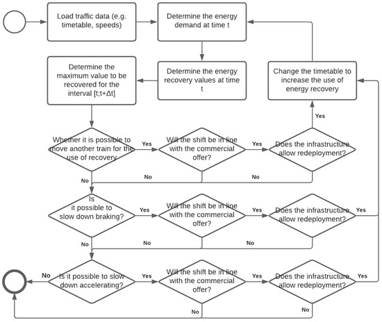
Figure 3.
A timetable reconfiguration algorithm that takes into account the increased level of consumption of recovered electricity.
In the first step of the algorithm, information in the area of infrastructure restrictions (speed, traffic methods, the energy consumption of vehicles, etc.) and the planned timetable and regulations within the commercial offer (time intervals of permissible deviations from the assumed schedule) are read in. In a second step, the traction characteristics of the individual trains are used to determine the electricity demand as a function of time for the substation under consideration. In the next step, the planned energy recovery (based on braking characteristics) is determined as a function of time. Then, for an assumed time interval of length Δt, the time interval [t; t + Δt] for the maximum operation is determined. Furthermore, the movement of trains can sometimes be carried out without interfering with the timetable because of the possibility of using time reserves already accounted for at the stage of construction of the original railway operating schedule. However, this is only possible when the train is running as scheduled. For such a time interval, to the feasibility of shifting a train that is accelerating is verified (it has a greater energy demand represented by greater power consumption and consequently—a more significant current), because of limitations of its commercial offer (if it will be following the carrier’s assumption). If such an operation is possible, it is checked whether it is possible to realise a journey on the analysed section with regard to infrastructure limitations. If it is possible, the change in the timetable is implemented and the planned energy demand and the energy recovery value are determined again. If a change cannot be made, it is checked if it is possible to make changes to the energy recovery function, e.g., by slowing down the brakes (divided into phases). Such an operation will reduce the instantaneous energy recovered, but overall it will remain at a similar level—it will be spread over time. In this case, if such a prolongation of braking is in accordance with the commercial offer and if it is feasible on the infrastructure section are also checked (if it will affect the system’s immunity to disturbances). If such an operation is possible, a braking deceleration is scheduled in the timetable in order for another train to use the energy recovered from the extended braking. In case such an operation does not make sense, the last step of the algorithm is implemented, i.e., checking if it is possible to slow down the acceleration (which will change the characteristics of the electric-energy consumption). Whether the gradual deceleration is compatible with the assumptions of the carrier and if the infrastructure is available for the proposed change are also verified. If so, a train is introduced, which accelerates up to a specific assumed moment (i.e., the moment when the other train ceases to be a source of energy) and then travels at a constant speed until another train in a given supply section begins to brake. At this point, the train travelling at a continuous speed starts to accelerate. After the operation, the revised timetable is saved, and the energy demand and recovery at time t are redetermined. The timetable reconfiguration ends when no shifting procedures can be performed on any train and when the energy-recovery value after the change does not increase.
The use of such an algorithm allows for the rationalisation of the global electricity demand in several ways. The algorithm makes it possible to make changes not only in terms of changing the trajectory of trains, but also allows trains to be moved in time. Such functionality brings an additional benefit, linked only indirectly to the electricity demand to power the trains. The algorithm will return a similar result for similar traffic situations occurring during the day. This means, for example, that trains running in opposite directions will always be shifted in time to the same dependence of the trajectory of the first train on the trajectory of the second train. Additionally, if such situations are repeated during the day—the algorithm will return the same result. As a result, the proposed algorithm will spontaneously tend to introduce a cyclic timetable. Using such an algorithm in Poland—a country in which attempts to introduce cyclic timetable on railways have failed for many years—would accelerate a transition to the cyclic timetable.
4. Results and Discussion
In this part of the paper, the proposed method will be verified. Section 4.1 discusses the boundary conditions of the task. Section 4.2 presents the results of testing the non-reconfigured schedule. Section 4.3 presents the results of the proposed algorithm and Section 4.4 of this thesis compares the distribution before and after reconfiguration.
It should be noted that—due to the multitude of calculations and results—the authors decided to show only a part of the calculations in this article.
The method was applied de facto for the following three train timetables: for weekdays (highest agglomeration traffic load, large number of regional and fast trains), Saturdays (lowest traffic) and Sundays and holidays (low share of agglomeration traffic, large number of regional and fast trains).
However, this paper only presents the results of the proposed method for the working timetable in detail, only for the hours 3:00 p.m. to 6:00 p.m. Nevertheless, the results for the other timetable hours and the other days are included in the comparison at the end of the chapter.
4.1. Case Study Boundary Conditions
In order to verify the method, a global energy intensity analysis was conducted before and after applying the proposed algorithm for a railway line with mixed traffic. For this purpose, a part of a route leading from Wrocław Główny towards Katowice (Poland) was used. This line combines the running of agglomeration transport within an urban centre of almost one million inhabitants, but at the same time is one of the most important interregional trunk routes in the country. In addition, there is occasional freight traffic on this line—although there is a parallel line dedicated to freight, so freight trains on this line make little use of it. A timetable that included trains with the parameters in Table 3 was analysed. Five of the supply sections with the most heavily loaded in rush hours (between 3:00 p.m. and 6:00 p.m.) in terms of traffic were selected. The selected sections are located closest to Wrocław.
Table 3.
Main characteristics of trains running on the railway line.
The parameters of the rail vehicles defined above and the mapping of the railway line provided a satisfactory result for the reproduction of the existing timetable. The results obtained from the theoretical runs—after adding the time reserves according to the regulations and after taking into account the duration of stops at passenger stops and stations—coincide with the times specified in the actual timetable.
4.2. Energy System Load Analysis before Timetable Reconfiguration
The simulation results that identify the situations that could be affected by the method proposed in this paper are presented in Figure 4. Due to the diversity of the data, only the results for one power section are shown as a representation. Negative values represent the current that can be transferred from a braked vehicle to other trains, after considering the energy-recovery efficiency, according to ref. [17]. The authors use current (instead of power) in their analyses due to its convenient form to convert the value into a parameter of electric current pacing.
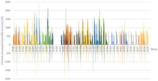
Figure 4.
Extract from the results obtained for the timetable simulation in the variant before reconfiguration.
A graph showing the global power consumption measured at the electrical substation (for non-negative values) and the recoverable power is presented below in Figure 5. The values have been ranked from highest to lowest. As this is a P(t) diagram, the area under the curve indicates the total electric power demand of the trains travelling along the section of the railway line under consideration.
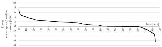
Figure 5.
Power consumption/possible recovery in the variant before reconfiguration.
The basic data characterising this option are summarised in Table 4 below.
Table 4.
Characteristics of variant before timetable reconfiguration.
Data prepared in this way allows for a further comparison between the variant before and after the reconfiguration of the train timetable.
4.3. Application of the Proposed Algorithm
The next step of the procedure is to apply the reconfiguration algorithm. To better explain the operation of the algorithm, the authors extensively discuss the results of introducing changes in the case of four traffic situations. At the same time, an analysis similar to that for the variant before reconfiguration was performed.
During the analysis of the traffic diagram for the mentioned sections of the railway line, several traffic situations were perceived which could potentially be rationalised in terms of reducing energy intensity. The application of the method proposed by the authors will be considered for four sample cases (which become scenarios) shown in Figure 6.
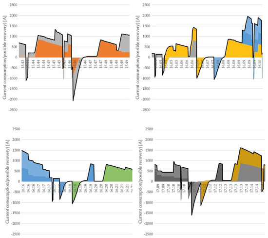
Figure 6.
Extract from the results obtained for the timetable simulation.
In scenario one, there are two trains within the limits of the supply section: a long-distance (orange) and a local (grey). The vehicles have overlapping times where braking occurs. Scenario two assumes the occurrence of a maximum of three trains in the supply section. However, four crossings are recorded in five minutes, including two passenger trains (yellow and light blue), one long-distance (dark blue) and one freight (grey). The next traffic situation identified, defined as scenario three, determines the occurrence of three trains, of a long-distance train stopping (dark blue), a freight train crossing the railway line in gear (light blue) and a local train (green). Scenario four involves up to three trains at a time, all of which are passenger trains. The black line indicates the energy balance for each time t. If the balance is negative, it is possible to give up energy at any time. If the balance is positive, there is the possibility to take up braking energy. The scenarios depicted graphically reveal the numerous occurrences of situations in which the braking of a single trainset takes place within a short time interval, often during one, two or three minutes. In detail, the effects of the algorithm are summarised in Table 5.
Table 5.
Results of the algorithm for the four revealed scenarios.
In the case of scenario one, the application of the method that is the subject of this article provided as a solution the shifting of the local train 94 s later and the slowing down of the braking process at its initial stage. Scenario two, after energy rationalisation, changed in such a way that the freight train was shifted by 21 s (shift to a later hour). The algorithm thus ensured that the energy recovered from breaking the local train, marked in yellow, was used. What is more, the algorithm also resulted in the long-distance train being postponed by 42 s. This ensures that the braking energy of this train can be recovered to accelerate the local (yellow) train. For scenario 3, the effect of the algorithm is to postpone the green train by 32 s. This action ensures that the braking energy of this train is used to accelerate the long-distance train. The most evident rescheduling occurs in scenario 4, where the algorithm proposes bringing the dark grey train (local train 1) 44 s forward (to accumulate energy demand with the brown train) and the light grey train (local train 2) 2 min 16 s forward, to allow the braking energy to be used to accelerate the other two trains (local trains 1 and 3).
Running the algorithm for just the four traffic situations indicated savings of 64.65 kWh. The average use of energy recoverable by the algorithm was 92.05%.
Below is a graph (Figure 7) showing the power consumption for modal loads occurring for the post reconfiguration option.
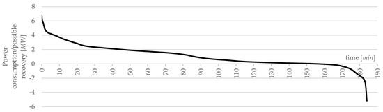
Figure 7.
Power consumption/possible recovery in the variant after reconfiguration by the proposed algorithm.
As in the case of the variant, before the proposed method was applied, the data obtained were collected in the form of a table (Table 6).
Table 6.
Characteristics of variant after timetable reconfiguration.
4.4. Comparison of Variants
Only by comparing the two options can it be established whether the use of the proposed method is justified. The table below (Table 7) performs such a comparison.
Table 7.
Comparison of the variants before and after reconfiguration by the proposed method.
It is clear from the data presented that it is reasonable to apply this reconfiguration method. It was found that it is possible to achieve a global energy demand reduction of up to about 398 MWh/year. However, this is a value determined not only for a specific time of day and only for the working timetables, but for the entire line, the entire good and each day of the week (distinguishing between weekdays, Saturdays and Sundays and holidays). The authors see further room for the development of the proposed method, including a consideration of issues related to the occurrence of traffic disruptions (train delays).
5. Conclusions
Researchers in various countries have addressed the problem of ensuring railways become more energy efficient. They have proposed different methods of reducing energy intensity in their work. However, the current state of knowledge did not take into account the preparation of a way based on algorithmics. A method that would combine—through algorithmics—the possibility of transferring the energy recovered during the braking of one train set to the power supply of accelerating trains with the possibility of manipulating—within the available time reserves—the trajectory of vehicle movement.
This work presents a method by which the global demand for electricity from railways can be influenced by designing timetables in a way that takes this aspect into account. The right decisions, adopted by applying the proposed method while still in the construction phase of the railway working plan, can contribute to achieving tangible benefits that are very much in keeping with the challenges posed by modern times. The authors recognise that there is room for further algorithm development to further improve the method. Disturbing traffic, for example, can be taken into account.
The authors point out the benefits of their proposed method not only in terms of reducing the energy intensity of rail transport. They also point out that the proposed algorithm returns timetables in such a form that it is possible to build cyclic timetables more easily.
Author Contributions
Conceptualisation, A.K. and S.H.; methodology, A.K. and S.H.; software, S.H.; validation, A.K.; formal analysis, A.K.; investigation, S.H.; resources, S.H.; data curation, S.H.; writing—original draft preparation, A.K. and S.H.; writing—review and editing, A.K.; visualisation, S.H.; supervision, A.K.; project administration, A.K.; funding acquisition, A.K. All authors have read and agreed to the published version of the manuscript.
Funding
This research received no external funding.
Institutional Review Board Statement
Not applicable.
Informed Consent Statement
Not applicable.
Data Availability Statement
Data are contained within the article.
Conflicts of Interest
The authors declare no conflict of interest.
References
- Heinold, A. Comparing emission estimation models for rail freight transportation. Transp. Res. Part D Transp. Environ. 2020, 86, 102468. [Google Scholar] [CrossRef]
- European Parliament and Council. Directive 2014/94/EU of the European Parliament and of the Council of 22 October 2014 on the Deployment of Alternative Fuels Infrastructure; European Parliament and Council: Brussels, Belgium, 2021. [Google Scholar]
- International Energy Agency. The Future of Rail: Opportunities for Energy and the Environment. 2019. Available online: https://www.iea.org/reports/the-future-of-rail (accessed on 22 November 2021).
- European Commission. 144 Wight Paper: Roadmap to a Single European Transport Area—Towards a Competitive and Resource Efficient Transport System; European Commission: Brussels, Belgium, 2011. [Google Scholar]
- Wang, P.; Goverde, R. Multi-train trajectory optimisation for energy efficiency and delay recovery on single-track railway lines. Transp. Res. Part B Methodol. 2017, 105, 340–361. [Google Scholar] [CrossRef]
- Vaneeckhaute, C.; Remigi, E.; Tack, F.M.G.; Meers, E.; Belia, E.; Vanrolleghem, P.A. Optimising the configuration of integrated nutrient and energy recovery treatment trains: A new application of global sensitivity analysis to the generic nutrient recovery model (NRM) library. Bioresour. Technol. 2018, 269, 375–383. [Google Scholar] [CrossRef] [PubMed]
- De Martinis, V.; Gallo, M. Models and Methods to Optimise Train Speed Profiles with and without Energy Recovery Systems: A Suburban Test Case. Procedia Soc. Behav. Sci. 2013, 87, 222–233. [Google Scholar] [CrossRef][Green Version]
- Polish Railway Transport Agency (Urząd Transportu Kolejowego). Passenger Exchange in 2019, Operation of Railways in the Voivodeships. Available online: https://utk.gov.pl/pl/dokumenty-i-formularze/opracowania-urzedu-tran/16623,Wymiana-pasazerska-w-2019-r.html (accessed on 10 December 2021).
- Khodaparastan, M.; Mohamed, A.A.; Brandauer, W. Recuperation of Re-generative Braking Energy in Electric Rail Transit Systems. IEEE Trans. Intell. Transp. Syst. 2019, 20, 2831–2847. [Google Scholar] [CrossRef]
- Cascetta, F.; Cipolletta, G.; Femine, A.D.; Fernández, J.Q.; Gallo, D.; Giordano, D.; Signorino, D. Impact of a reversible substation on energy recovery experienced onboard a train. Measurement 2021, 183, 109793. [Google Scholar] [CrossRef]
- Żurek, Z.H.; Duka, P. Obciążalność Prądowa Sieci Trakcyjnej Systemu 3kV w Świetle Zwiększania Mocy i Prędkości. Pr. Nauk. Politech. Warsz. Transp. 2017, 119, 529–539. [Google Scholar]
- Popescu, M.; Bitoleanu, A. A Review of the Energy Efficiency Improvement in DC Railway Systems. Energies 2019, 12, 1092. [Google Scholar] [CrossRef]
- Lin, X.; Wang, Q.; Wang, P.; Sun, P.; Feng, X. The Energy-Efficient Operation Problem of a Freight Train Considering Long-Distance Steep Downhill Sections. Energies 2017, 10, 794. [Google Scholar] [CrossRef]
- Radu, P.V.; Szelag, A.; Steczek, M. On-Board Energy Storage Devices with Supercapacitors for Metro Trains—Case Study Analysis of Application Effectiveness. Energies 2019, 12, 1291. [Google Scholar] [CrossRef]
- Arboleya, P.; El-Sayed, I.; Mohamed, B.; Mayet, C. Modeling, Simulation and Analysis of On-Board Hybrid Energy Storage Systems for Railway Applications. Energies 2019, 12, 2199. [Google Scholar] [CrossRef]
- Hillmansen, S.; Ellis, R. Electric railway traction systems and techniques for energy saving. In Proceedings of the IET 13th Professional Development Course on Electric Traction System, London, UK, 3–6 November 2014. [Google Scholar]
- Cipolletta, G.; Delle Femine, A.; Gallo, D.; Luiso, M.; Landi, C. Design of a Stationary Energy Recovery System in Rail Transport. Energies 2021, 14, 2560. [Google Scholar] [CrossRef]
- Dominguez, M.; Fernández-Cardador, A.; Cucala, A.P.; Pecharroman, R.R. Energy Savings in Metropolitan Railway Substations Through Regenerative Energy Recovery and Optimal Design of ATO Speed Profiles. IEEE Trans. Autom. Sci. Eng. 2012, 9, 496–504. [Google Scholar] [CrossRef]
- Su, S.; Wang, X.; Cao, Y.; Yin, J. An Energy-Efficient Train Operation Approach by Integrating the Metro Timetabling and Eco-Driving. IEEE Trans. Intell. Transp. Syst. 2020, 21, 4252–4268. [Google Scholar] [CrossRef]
- Morea, D.; Elia, S.; Boccaletti, C.; Buonadonna, P. Improvement of Energy Savings in Electric Railways Using Coasting Technique. Energies 2021, 14, 8120. [Google Scholar] [CrossRef]
- Ghoseiri, K. A New Idea for Train Scheduling Using Ant Colony Optimization. WIT Trans. Built Environ. 2006, 8, 9. [Google Scholar]
- Samà, M.; D’Ariano, A.; Pacciarelli, D.; Pellegrini, P.; Rodriques, J. Ant colony optimization for train routing selection: Operational vs tactical application. In Proceedings of the 5th IEEE International Conference on Models and Technologies for Intelligent Transportation Systems (MT-ITS), Naples, Italy, 26–28 June 2017; Volume 5, pp. 297–302. [Google Scholar]
- Montrone, T.; Pellegrini, P.; Nobili, P.; Longo, G. Energy consumption minimisation in Railway Planning. In Proceedings of the IEEE 16th International Conference on Environment and Electrical Engineering (EEEIC), Florence, Italy, 7–10 June 2016. [Google Scholar]
- Lu, Q.; He, B.; Wu, M.; Zhang, Z.; Luo, J.; Zhang, Y.; He, R.; Wang, K. Establishment and Analysis of Energy Consumption Model of Heavy-Haul Train on Large Long Slope. Energies 2018, 11, 965. [Google Scholar] [CrossRef]
- Rocha, A.; Araújo, A.; Carvalho, A.; Sepulveda, J. A New Approach for Real Time Train Energy Efficiency Optimization. Energies 2018, 11, 2660. [Google Scholar] [CrossRef]
- Wang, L.; Wang, X.; Liu, K.; Sheng, Z. Multi-Objective Hybrid Optimization Algorithm Using a Comprehensive Learning Strategy for Automatic Train Operation. Energies 2019, 12, 1882. [Google Scholar] [CrossRef]
- Bu, B.; Qin, G.; Li, L.; Li, G. An Energy Efficient Train Dispatch and Control Integrated Method in Urban Rail Transit. Energies 2018, 11, 1248. [Google Scholar] [CrossRef]
- Fernández-Rodríguez, A.; Fernández-Cardador, A.; Cucala, A.P.; Falvo, M.C. Energy Efficiency and Integration of Urban Electrical Transport Systems: EVs and Metro-Trains of Two Real European Lines. Energies 2019, 12, 366. [Google Scholar] [CrossRef]
- Chen, E.; Bu, B.; Sun, W. An Energy-Efficient Operation Approach Based on the Utilisation of Regenerative Braking Energy among Trains. In Proceedings of the IEEE International Conference on Intelligent Transportation Systems, Las Palmas, Spain, 15–18 September 2015; pp. 2606–2611. [Google Scholar]
- Gong, C.; Zhang, S.; Zhang, F.; Jiang, J.; Wang, X. An integrated energy-efficient operation methodology for metro systems based on a real case of Shanghai metro line one. Energies 2014, 7, 7305–7329. [Google Scholar] [CrossRef]
- Peña-Alcaraz, M.; Fernández, A.; Cucala, A.P.; Ramos, A.; Pecharromán, R.R. Optimal underground timetable design based on power flow for maximizing the use of regenerative-braking energy. Proc. Inst. Mech. Eng. Part F 2012, 226, 397–408. [Google Scholar] [CrossRef]
- Bu, B.; Ding, Y.; Li, C.; Mao, X. Research on integration of train control and train scheduling. J. China Railw. Soc. 2013, 35, 64–71. [Google Scholar]
- Madej, J. Teoria Ruchu Pojazdów Szynowych; Oficyna Wydawnicza Politechniki Warszawskiej: Warsaw, Poland, 2012. [Google Scholar]
- Kwaśnikowski, J. Elementy Teorii Ruchu i Racjonalizacja Prowadzenia Pociągu; Wydawnictwo Naukowe Instytutu Technologii Eksploatacji: Radom, Poland, 2013. [Google Scholar]
- Chwieduk, A.; Dyr, T. Projektowanie Ruchu Pociągów; Zakład Poligraficzny Politechniki Radomskiej: Radom, Poland, 1997. [Google Scholar]
- Wyrzykowski, W. Ruch Kolejowy; Wydawnictwa Komunikacji: Sulejówek, Poland, 1951. [Google Scholar]
- PKP Polskie Linie Kolejowe SA. Instrukcja o Rozkładzie Jazdy Pociągów (Ir-11); PKP Polskie Linie Kolejowe Institution: Warsaw, Poland, 2015. [Google Scholar]
Publisher’s Note: MDPI stays neutral with regard to jurisdictional claims in published maps and institutional affiliations. |
© 2022 by the authors. Licensee MDPI, Basel, Switzerland. This article is an open access article distributed under the terms and conditions of the Creative Commons Attribution (CC BY) license (https://creativecommons.org/licenses/by/4.0/).