Article

Using Transfer Learning to Build Physics-Informed Machine Learning Models for Improved Wind Farm Monitoring

by
Laura Schröder
1,*,
Nikolay Krasimirov Dimitrov
1,
David Robert Verelst
1 and
John Aasted Sørensen
2
1
DTU Wind Energy, Technical University of Denmark, 4000 Roskilde, Denmark
2
DTU Engineering Technology, Technical University of Denmark, 2750 Ballerup, Denmark
*
Author to whom correspondence should be addressed.
Energies 2022, 15(2), 558; https://doi.org/10.3390/en15020558
Submission received: 19 October 2021 / Revised: 23 December 2021 / Accepted: 4 January 2022 / Published: 13 January 2022
(This article belongs to the Collection Women's Research in Wind and Ocean Energy)

Abstract

:
This paper introduces a novel, transfer-learning-based approach to include physics into data-driven normal behavior monitoring models which are used for detecting turbine anomalies. For this purpose, a normal behavior model is pretrained on a large simulation database and is recalibrated on the available SCADA data via transfer learning. For two methods, a feed-forward artificial neural network (ANN) and an autoencoder, it is investigated under which conditions it can be helpful to include simulations into SCADA-based monitoring systems. The results show that when only one month of SCADA data is available, both the prediction accuracy as well as the prediction robustness of an ANN are significantly improved by adding physics constraints from a pretrained model. As the autoencoder reconstructs the power from itself, it is already able to accurately model the normal behavior power. Therefore, including simulations into the model does not improve its prediction performance and robustness significantly. The validation of the physics-informed ANN on one month of raw SCADA data shows that it is able to successfully detect a recorded blade angle anomaly with an improved precision due to fewer false positives compared to its purely SCADA data-based counterpart.

1. Introduction

Wind power remains one of the fastest growing renewable energy sources with a global installed wind power capacity of 744 GW by the end of 2020 [1]. With the continued trend of the growing wind turbine (WT) size and their deployment in offshore environments, it becomes increasingly important to reduce the operation and maintenance (O&M) costs by optimizing O&M activities. In this context, monitoring and predicting the turbine performance plays an important role for enabling the implementation of predictive maintenance strategies. Studies have shown that underperformance, e.g., due to pitch faults or gearbox faults, can lead to significant losses in the revenues [2]. It is therefore important for the operators to deploy intelligent monitoring of the wind turbines health state, termed condition monitoring (CM), to reduce unscheduled downtime and thus operational costs of wind energy [3]. The aim of CM is to detect deviations from the normal operational behavior indicating a developing fault. This requires detailed knowledge of the system, which is often not available. Traditional dedicated condition monitoring systems (CMS) are mostly based on extra measurements (e.g., vibration measurements, strain measurements, thermography and acoustic emissions) which makes them costly since they require the installation of extra sensors.
However, utility-scale turbines are typically equipped with a standard supervisory control and data acquisition (SCADA) system. Using the SCADA data for condition monitoring purposes has become more and more popular as it presents a low-cost alternative to the CMS solutions. An extensive review of the various approaches which have already proved successful in detecting anomalies using the turbine data can be found in [4].
Most of recent research focuses on normal behavior modeling (NBM) in which a model is trained to predict a specific output signal using historic SCADA data from periods where the turbine is considered to operate under healthy conditions. After the training phase, the model can be applied to estimate the output signal. The residual of the modeled minus the measured variable serves as indicator for an anomaly from normal operation. The important advantages of the purely data-driven NBM method are that no prior knowledge about the signal behavior is needed [3] and monitoring the residual for anomaly detection is mostly decoupled from the turbines operational mode [5].
Models based on machine learning methods, especially artificial neural networks (ANN) have shown good anomaly detection abilities [4]. However, the disadvantage of such black-box models is that they are difficult to interpret and require a large amount of data. Furthermore, the training of purely data-driven models can be affected by noise of measurements, and although it seems to perform well on training and test data, it might lead to poor generalization outside the available data. With the recent trend of increased computing power, it becomes feasible to combine physics with ML in different ways, which is recognized as the term “theory-guided data science”, “physics-guided machine learning” or also “physics-informed machine learning”. Including physics information into ML detection models may enable learning generalizable patterns without overfitting.
In [6], the authors present an extensive taxonomy overview of the different ways knowledge can be included in a machine learning system. Due to the reasons mentioned above, there is a lot of interest by both research and industry in the wind sector to build more robust models by leveraging physics-informed machine learning. However, there is only little research on such physics-informed ML techniques applied to wind turbine CM: For an automatic diagnosis of the observed residual patterns in the NBM procedure, expert knowledge can be incorporated by using fuzzy inference systems based on a set of if-then rules, as shown in [3,7,8]. In [9], a physics-informed Gaussian process approach is developed that can be used for detecting power grid faults. For the application of damage modeling, a physics-informed neural network is built based on repeating cells of recurrent neural networks (RNNs) in [10,11].

1.1. Objective

However, these approaches have not been applied to the commonly used NBM. Especially, in situations where SCADA data are scarce or noisy, it might not be enough to build a well-performing NBM based solely on measurement data. Therefore, this study investigates the potential of augmenting SCADA data with aeroelastic simulations for building NBM models of wind turbines in a wind farm by means of a knowledge transfer technique called transfer learning. The hypothesis to be tested is on whether including physics constraints in this way improve the performance of the normal behavior model and its corresponding anomaly detection when having a limited amount of SCADA data. The model improvement is measured by the following performance metrics:
  • Sample efficiency (i.e., how much data are needed to reach a certain prediction accuracy)
  • Robustness (i.e., how much the prediction error varies)
  • Ability to detect anomalies (i.e., precision and recall)

1.2. Paper Outline

The remainder of the article is structured as follows: In Section 2, the concept of the proposed method for including physics knowledge into a deep-learning-based normal behavior model is described. Two different methods for augmenting SCADA data with simulations, as well as their usage for anomaly detection, are explained. In Section 3, the described concept is applied to the SCADA data from an offshore wind farm. The resulting model performances are shown for different amounts of SCADA data used and different amounts of knowledge transferred. These results are compared against their purely data-driven counterparts. Moreover, the residual analysis of the models applied to raw SCADA data for anomaly detection is presented. Section 4 compares the presented methods and discusses its limitations, i.e., under which specific conditions is augmenting data-driven monitoring models with simulations beneficial for a turbine operator. Furthermore, the impact on the suggested approach on the anomaly detection ability is discussed. In Section 5, the conclusions of this study are drawn, and future work is suggested.

2. Materials and Methods

The normal behavior model monitors the SCADA data via a set of input signals and is built using the following steps: (1) data preparation, (2) model training and model evaluation and (3) residual analysis. In the first step, the SCADA data are preprocessed and filtered to select a subset which represents normal WT operations without faults. If alarm logs of the SCADA system are available, they can be used for flagging any observation deviating from normal operation, i.e., faulty, transient, curtailed, etc. A regression model is then trained and evaluated on the normal behavior SCADA data. After the training phase, the evaluated model is applied to new raw SCADA data to estimate the to-be-monitored output signal. The estimated output is compared against the actual measured signal, and the residual pattern is analyzed in order to detect anomalies. Typically, this involves setting a threshold which, if exceeded, would indicate an anomaly.

2.1. Transfer Learning for NBM

The aim of transfer learning is to improve the performance of a target learner on a target domain D T by transferring knowledge contained in a different but related source domain D s [12,13] (see Figure 1). A recent comprehensive review on transfer learning can be found in [13].
The SCADA database used for building the normal behavior monitoring model represents our target domain data D T = { X T , P T ( X T ) } with a feature space X T and a distribution P T ( X T ) , whereas a large simulation database serves as the source domain data D S = { X s , P S ( X S ) } with a corresponding feature space X S and distribution P S ( X S ) .
A source model trained on a large number of aeroelastic simulations is assumed to capture the main physics behavior of the turbine operation under the simulated conditions. As the turbines’ measurement data are limited, the idea is to introduce physics constraints by using the knowledge obtained in the pretrained source model to improve the performance of the target model.

2.2. Feature Selection

This study focuses on a turbine which is located in an offshore wind farm. Since the turbine operates under the influence from the wakes of neighboring turbines, features capturing these influences need to be used in the model. As the electrical power P is the main characteristic for describing the overall operation of a WT, it is used as output of the normal behavior model in this study. Only inputs that are available in both measurement and simulation data are used for modeling the power of a turbine in a wind farm. Based on a previous study [14], the selected input variables are the wind speed u, the wind speed standard deviation σ u , the row spacing R D , wake incidence angle γ and number of disturbing turbines N r o w s :
X m o d e l = [ u , σ u , R D , γ , N r o w s ]
The wake experienced by the monitored turbine can be characterized by the latter three variables ( R D , γ , N r o w s ). This is based on its relative position towards the other wake sources within the wind farm. More details on the input selection can be read in [14].

2.3. Creation of Source Data (Simulation)

The simulation database is created by carrying out a 30,000 point Monte Carlo (MC) simulation with samples drawn from the joint probability distribution of the defined input variable space X s i m . Selecting this input variable space is an important step in the creation of the simulation data. The choice of input variables and their probability distributions is based on the intention to cover a wide range of environmental conditions that are representative for the wind farm used in this study. Further details about the input variable distributions and their boundary functions can be found in a previous study by the authors in which the database has been created [15].
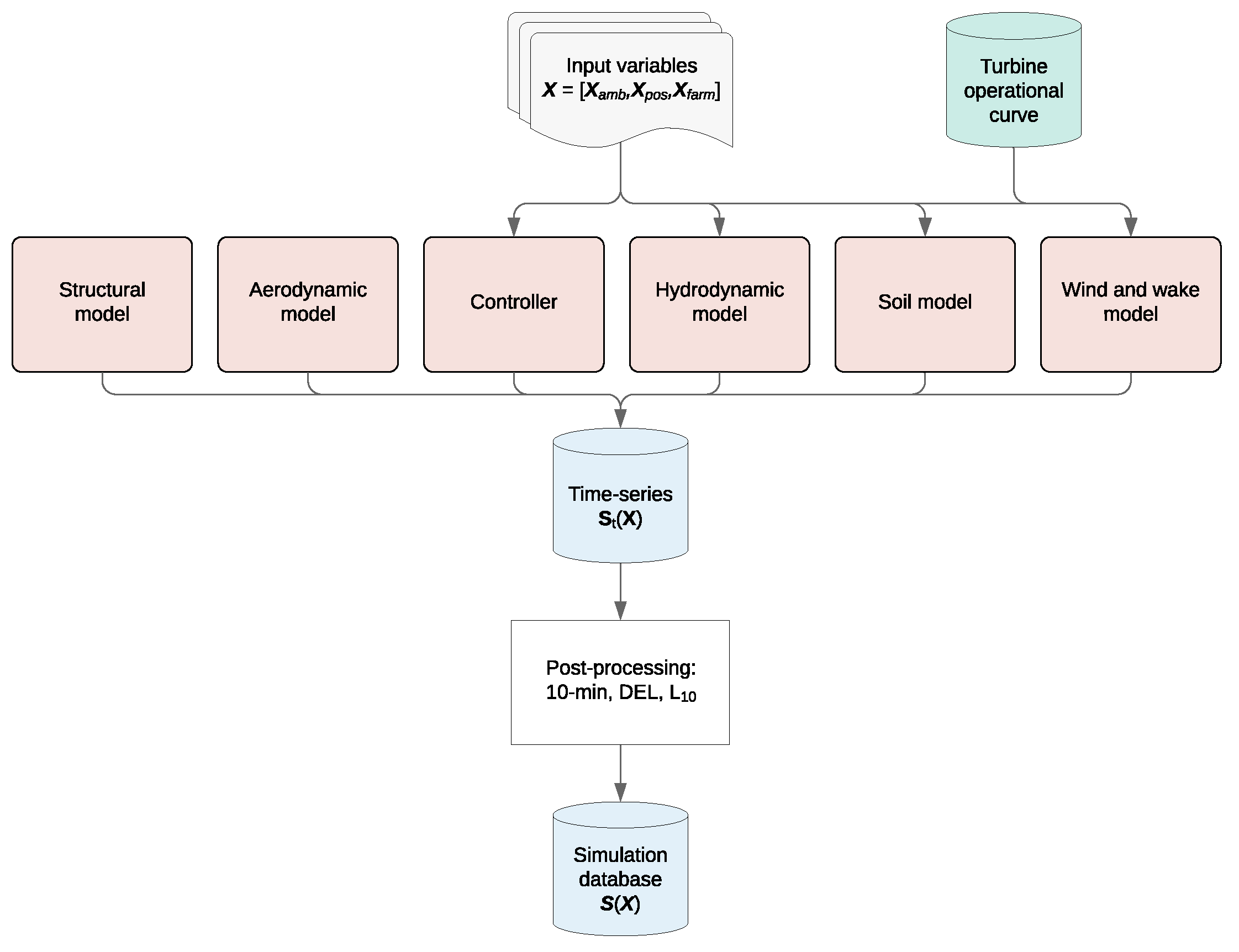
Figure 2 presents the set of models that are required to run aeroelastic time series simulations S t ( X ) on the 30,000 input samples. In order to model the turbine response to the wind inflow conditions, a structural, aerodynamic, and controller model is required. For offshore turbines, additional models accounting for the hydrodynamic and soil forces are to be considered as well. In this study, the aeroelastic tool HAWC2 [16,17] is used to simulate a turbine under normal operating conditions. This means that the simulations are carried out for normal power production (i.e., not for start-up or shutdown behavior and without faults) for wind speeds in the entire operational range of the turbine. The stochastic part of the wind is modeled using the Mann spectral turbulence generator [18]. In this way, time series that are generated for the same conditions are different for each realization. This variability causes uncertainty in the turbine performance. However, the uncertainty for the performance estimation through the variability of the wind is reduced by using a large Monte Carlo sample [15]. The dynamic wake meandering (DWM) model [19] is used for simulating the wake effects from multiple wake sources N r o w s .
Finally, the time series simulations S t ( X ) are postprocessed in order to calculate the 10 min statistics. The interested reader can find further details about the method and specific simulation set up in [15]. The database is openly available in https://doi.org/10.11583/DTU.12245978 (accessed on 10 January 2022).

2.4. Method 1: Artificial Neural Network (Parameter Transfer)

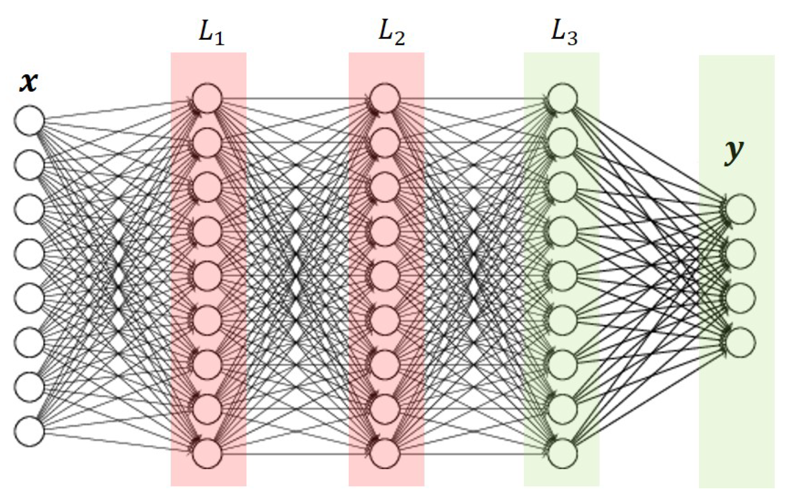
The first method used for training a normal behavior regression model is an artificial neural network (ANN). The ANN is selected due to its high potential for delivering fast and accurate predictions for a variety of applications, such as demonstrated in previous studies [5,20,21]. As illustrated in Figure 3, an ANN consists of a number of neurons which are organized in layers L. Its simplest form is a multilayer perceptron (MLP), in which the input vector x is processed forward through the hidden layers to calculate and output vector y . Figure 3 shows a network with three hidden layers and input and output vectors as used in this study.
At each neuron j, the n-dimensional input is processed with a linear transfer function:
a j = i = 1 n w j i x i + w j 0
with the weight parameter w i and the bias parameter w 0 . The result a j is then passed through a nonlinear activation function:
z j = h ( a j )
The output z j of neuron j then serves as input to the neurons of the following layer until the output layer is reached. The parameters of the network are trained using a back-propagation algorithm and an optimization algorithm that minimizes a loss function. In this case, a least-squares cost function is used to minimize the loss:
L o s s ( w ) = 1 2 f ( x , W ) y ( x ) 2
In order to add physics constraints into the training of a normal behavior network, a network that is pretrained on the source data (simulations) is used as a starting point for the new training task on the SCADA data. For the latter, the weight parameters of the first n f i x e d layers are kept constant such that only parameters of the remaining layers are adjusted during the retraining phase on the SCADA data.

2.5. Method 2: Stacked Denoising Autoencoder (Subspace Transfer)

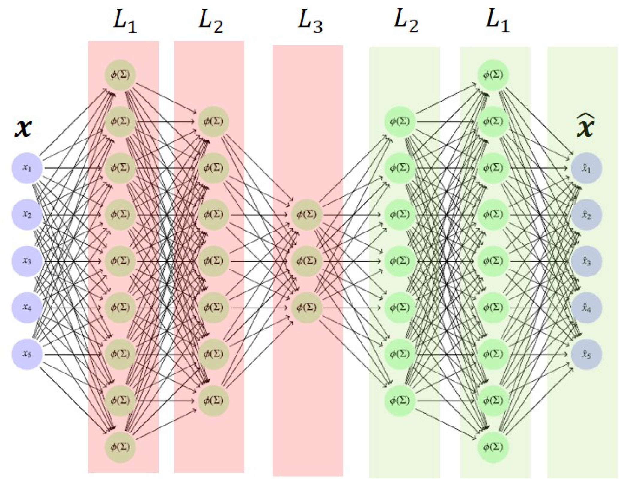
Secondly, an autoencoder (AE) is used as an alternative method for building a normal behavior model of the power. Previous studies have highlighted the promising use of denoising autoencoders for fault detection purposes with its advantages of strong learning abilities together with the decreased risk of overfitting [22,23]. A basic AE is a feed-forward neural network with one hidden layer, also called code layer, and the output vector being equal to the input vector. An AE is composed of an encoder function h = f ( x ) , which maps the input vector x to the code, and a decoder function x ^ = g ( h ) , mapping the code back to a reconstruction of the input x ^ . When multiple AE layers are stacked to form a deep learning network it is called a stacked auto encoder (SAE). Figure 4 shows an example of such a stacked autoencoder with the code layer L 3 and the remaining hidden layers L 1 and L 2 . By setting the size of the code layer to be smaller than the input dimension, the network is forced to model a compressed, lower-dimensional latent subspace Z. To make sure that the network does not simply reproduce the input signal, Gaussian noise is added to the input. This modified version of the AE is called a stacked denoising autoencoder (SDAE). Several studies used AEs as a regression model for WT monitoring [22,23].
Similarly to the above-described ANN knowledge transfer, a SDAE network is trained on the simulation data and retrained on SCADA data while keeping the parameters of the first n f i x e d layers constant. When keeping all layers up to the code layer fixed (see Figure 4), the hypothesis is that the subspace Z learned on the simulations helps the model to better learn the target task on the SCADA data.

2.6. Anomaly Detection

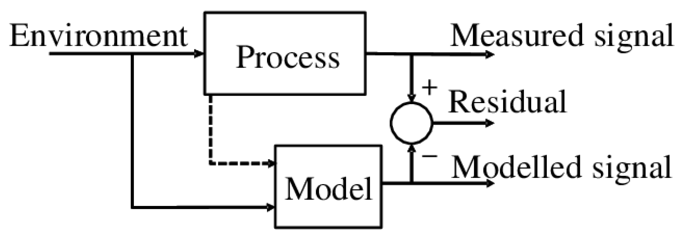
After training and evaluating the normal behavior models, they are applied to the raw SCADA data to estimate the power output. As presented in Figure 5, the power estimation y ^ is compared with the actual measured power y by calculating the residual ϵ :
ϵ = y ^ y
Large deviations between the measured and the modeled signal indicate abnormal behavior. When analyzing the residual for the detection, it is crucial to consider information about the uncertainty of the model estimates. The underlying assumption of anomaly detection is that normal observations are present in high probability regions and anomalies in low-probability regions of a stochastic model [3]. Therefore, the distribution of the power residuals during the testing phase of the normal behavior model are used for setting normal thresholds. Assuming that the testing residuals ϵ t e s t are normally distributed, the upper and lower control limits (CL) are calculated using the following equation based on [24]:
C L = μ t e s t ± η σ t e s t n
with the average prediction error μ t e s t , the standard deviation of prediction errors σ t e s t , and the number of observations n used for testing. The constant η is manually tuned in order to attain the confidence interval that avoids sensitivity toward data variations. A residual of the predictions on new SCADA observations that surpasses the control limits is assumed to have low probability based on the trained normal behavior model and is therefore detected as an abnormal observation.
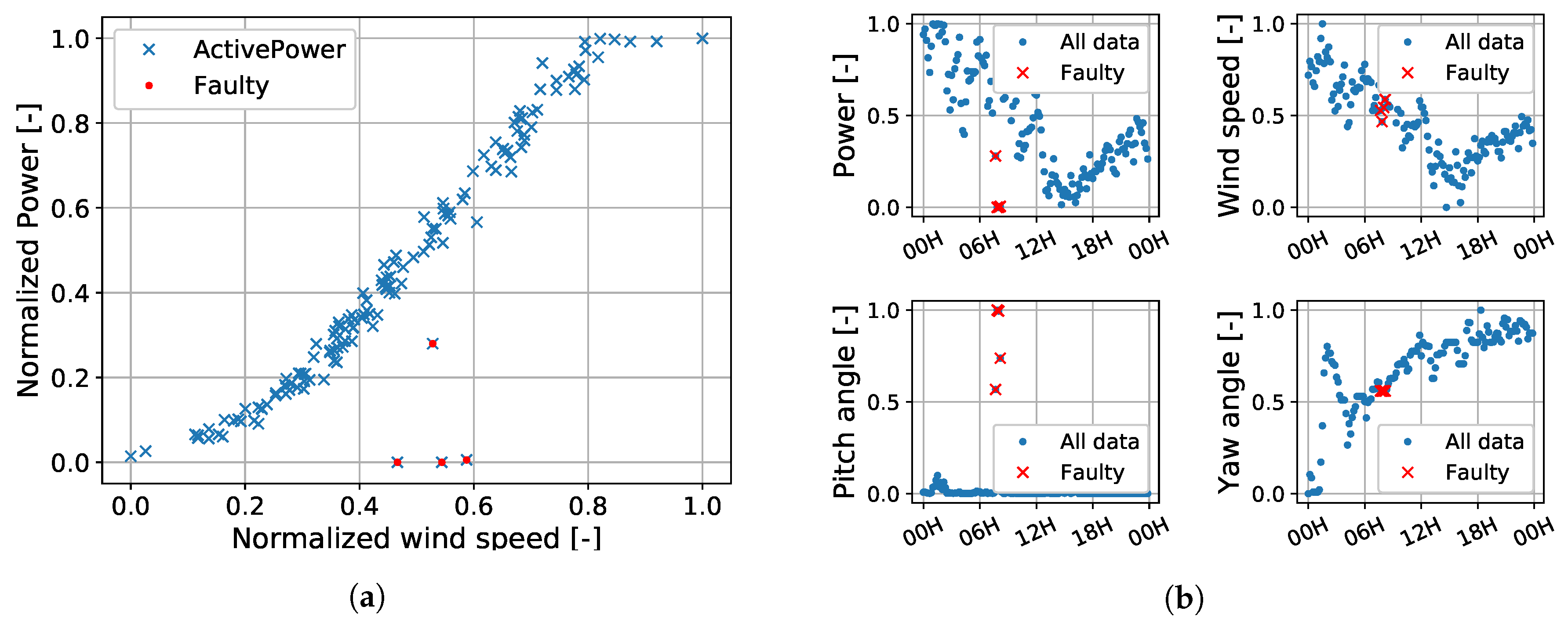
The detection ability of the normal behavior models was tested on one month of raw SCADA data (1 May to 31 May 2016). During this period, the SCADA system recorded an implausible blade angle on 21 May 2016 for a duration of 31 min. Figure 6 shows the power curve and time-series measurements of power, wind speed, pitch angle and rotor speed for the time window in which the alarm occurred. The signals are normalized by their maximum value.
To evaluate the performance of the anomaly detection system, the precision and recall are calculated. The precision of a binary classifier measures the probability that the detected anomaly is an actual anomaly and is defined as follows:
P r e c i s i o n = # T r u e P o s i t i v e s # T r u e P o s i t i v e s + # F a l s e P o s i t i v e s
The recall on the other hand, also known as sensitivity, indicates how well the system is able to find anomalies:
R e c a l l = # T r u e P o s i t i v e s # T r u e P o s i t i v e s + # F a l s e N e g a t i v e s
These performance metrics depend on how the normal threshold is defined. A low threshold results in a high recall where a large fraction of anomalies are detected; however, with a lower precision, more normal observations are flagged as an anomaly. A too high threshold gives the opposite result [22]. Therefore, setting a suitable threshold is a crucial task for building an anomaly detection system.

3. Results

3.1. Data Preparation

The SCADA data from an offshore wind farm with 305 MW turbines are available for the period from July 2011 to May 2017 with a sampling rate of 10 min. Furthermore, alarm logs of the SCADA system are available for the period from June 2012 to June 2017. The results are presented for a turbine located at the eastern border of the wind farm. With southwestern prevailing wind direction, the WT is mainly exposed to wake effects from three to four upstream turbines. This turbine is selected since it has one of the lowest downtime and lowest fault frequency within the wind farm and therefore contains a large amount of SCADA data for building a normal behavior model. Nevertheless, visualizations of the SCADA data and alarm logs show indications of underperformance issues for testing the monitoring models.
The alarms are processed and categorized into the component related subsystem following the reviewed taxonomy of modernized WT [25]. Only alarms that the authors consider as indications of a fault or problem are considered. The majority of the critical alarms are related to the rotor and blade subsystem. To the authors knowledge, the turbine did not experience any main bearing or gearbox failure for the recorded time.

3.2. SCADA Data (Target Domain)

The SCADA signals are synchronized and filtered to normal behavior. Firstly, all observations that are flagged as curtailed, not operating, transient or faulty by the SCADA system are discarded. Secondly, the OpenOA toolkit developed at NREL [26] is applied.

3.3. Simulation Data (Source Domain)

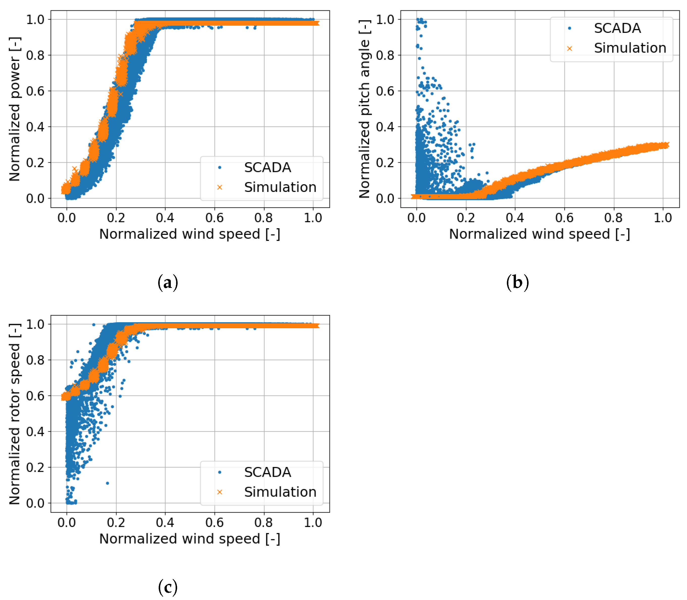
The source data are simulated as described in Section 2.3. The simulations are carried out using the NREL offshore 5MW reference turbine with a jacket structure model [27]. Figure 7 shows a comparison of the simulation results against the SCADA signals power, pitch angle and rotor speed with respect to the wind speed.

3.4. Model Performance Evaluation

In order to analyze the impact of augmenting simulations into the SCADA data under different data availabilities, the target normal behavior models were trained and tested using 1, 3, 6, 9 and 12 months of data, respectively. The available data were shuffled, and each model was trained on 80% of the data, whereas its prediction performance was tested on the remaining 20% of the data to avoid overfitting. Firstly, the data was shuffled, and each model was trained on 80% of the data and tested on the remaining 20% of data to avoid overfitting. This was performed within a five-fold crossvalidation for estimating the generalization error such that all of the available data points have been used for training once. The variation of the generalization error is an indicator for how robust the model performance with different training/test splits. Secondly, in order to properly compare the model performances with different amounts of training sizes, a model was trained completely on 1, 3, 6, 9 and 12 months of data and tested on the same subsequent 3 month period. Here, the prediction performance of each model set up was evaluated on three iterations in order to account for the performance variations due to randomness in the ANN (i.e., initialization).
For the performance evaluation, the coefficient of determination ( R 2 ) and the percentage of normalized root mean squared error (NRMSE) were calculated using the following equations:
R 2 = 1 S S r e s S S t o t = 1 i = 1 n ( y y ^ ) 2 i = 1 n ( y y ¯ ) 2
NRMSE [ % ] = 1 P r a t e d i = 1 n ( y ^ y ) 2 n · 100
with the mean of measured power y ¯ , rated power of the turbine P r a t e d and number of test observations n. The R 2 value represents how much variability of the output has been accounted for with the sum of squares of residuals S S r e s and the total sum of squares S S t o t , which is proportional to the variance of the data.
Both ANN and SDAE methods are implemented using the Sequential class of the Python deep-learning-library Keras, since the Sequential class allows one to keep selected parameters fixed during the retraining of the network.

3.5. Artificial Neural Network (Parameter Transfer)

After hyperparameter tuning, the most suitable network architecture for a SCADA-based ANN consists of three hidden layers with 25 neurons in each layer. The network is trained using the Adam optimization algorithm with a learning rate of 0.7 and a batch size of 400. A regularization factor of 0.001 is used to avoiding overfitting.
The source model is trained with 400 epochs on the complete simulation database. Figure 8 and Figure 9 show the model performance of the source model on the test data. The coefficient of determination of the predictions from the source model is 0.995, and the NRMSE is 2.35%.
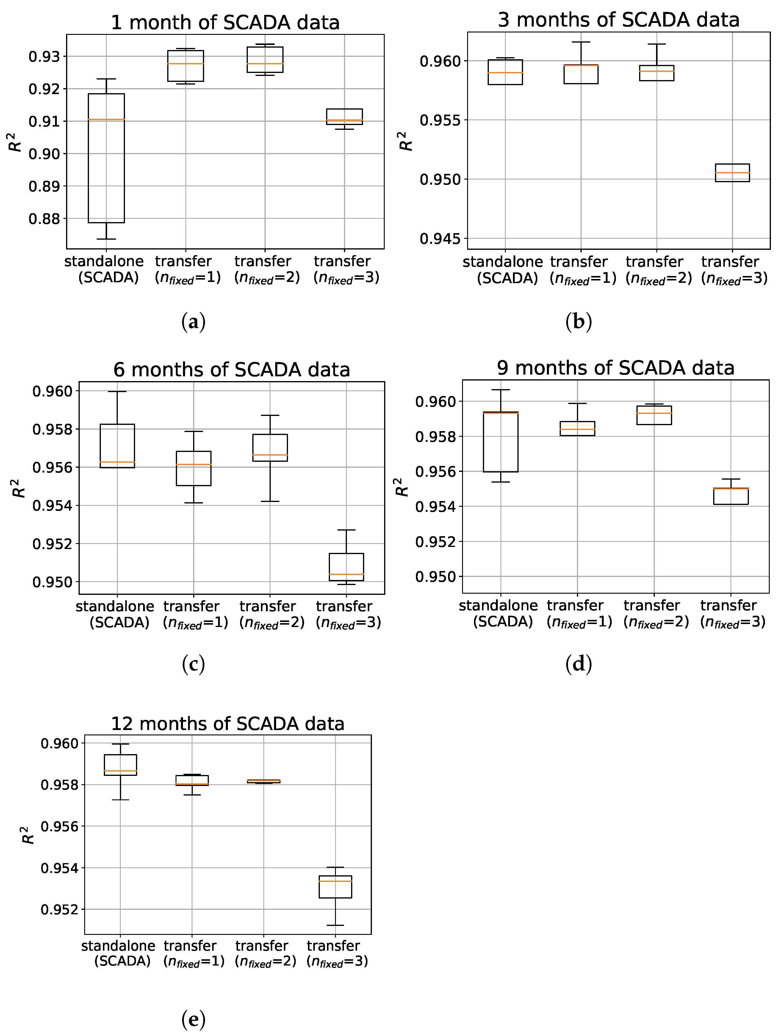
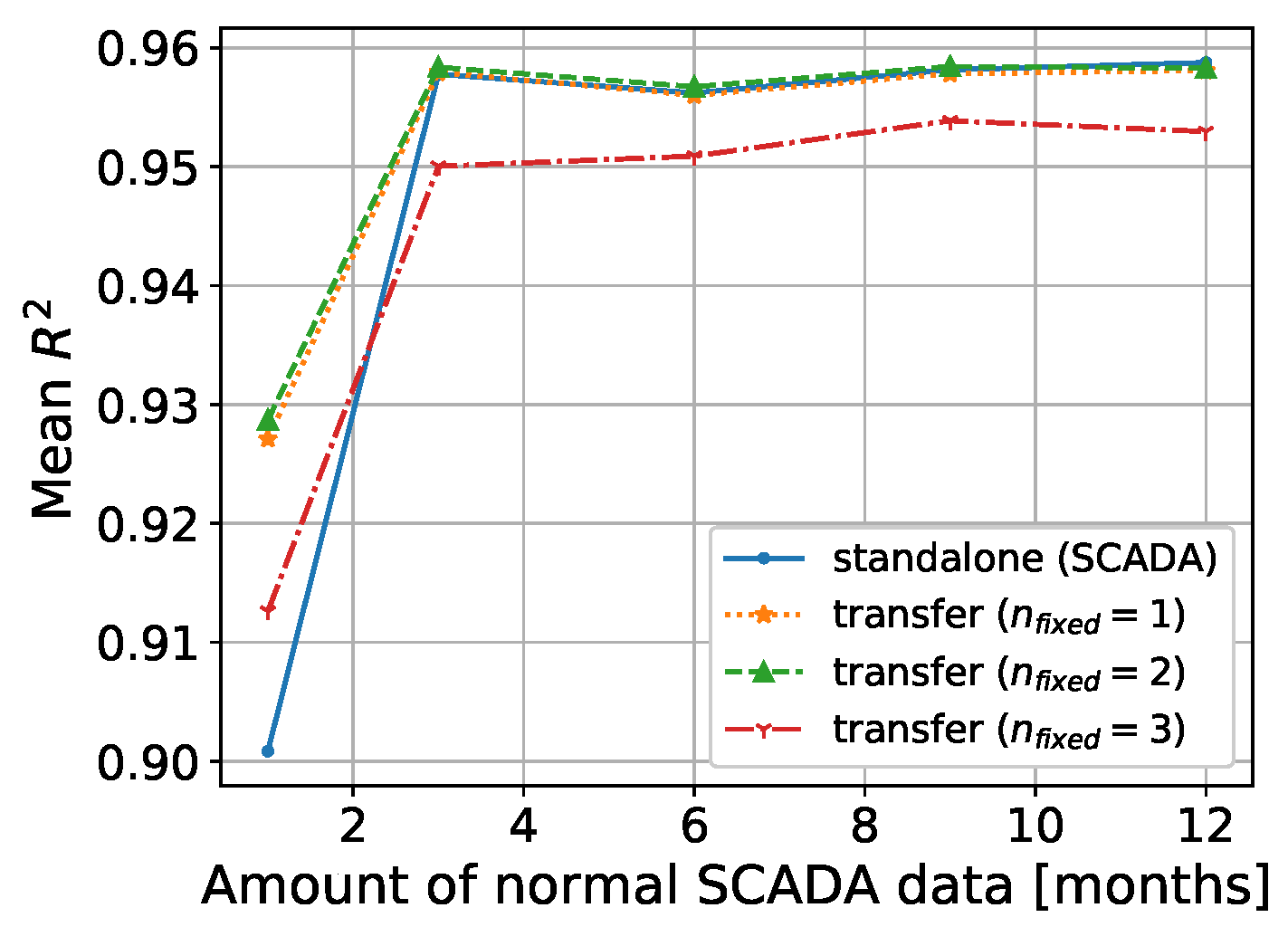
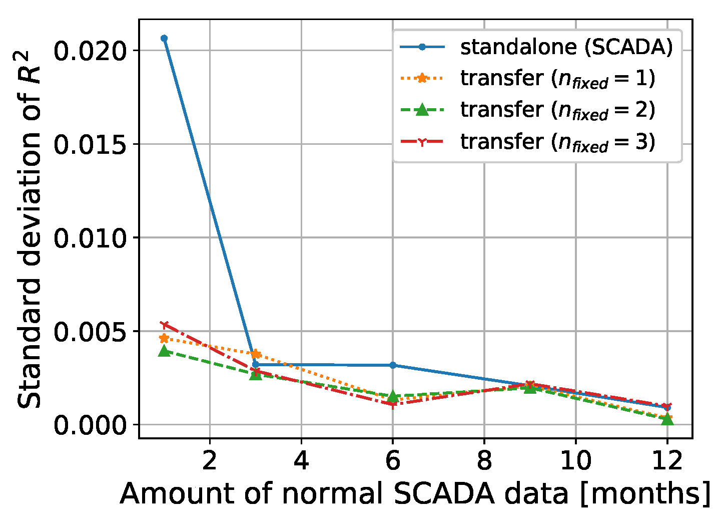
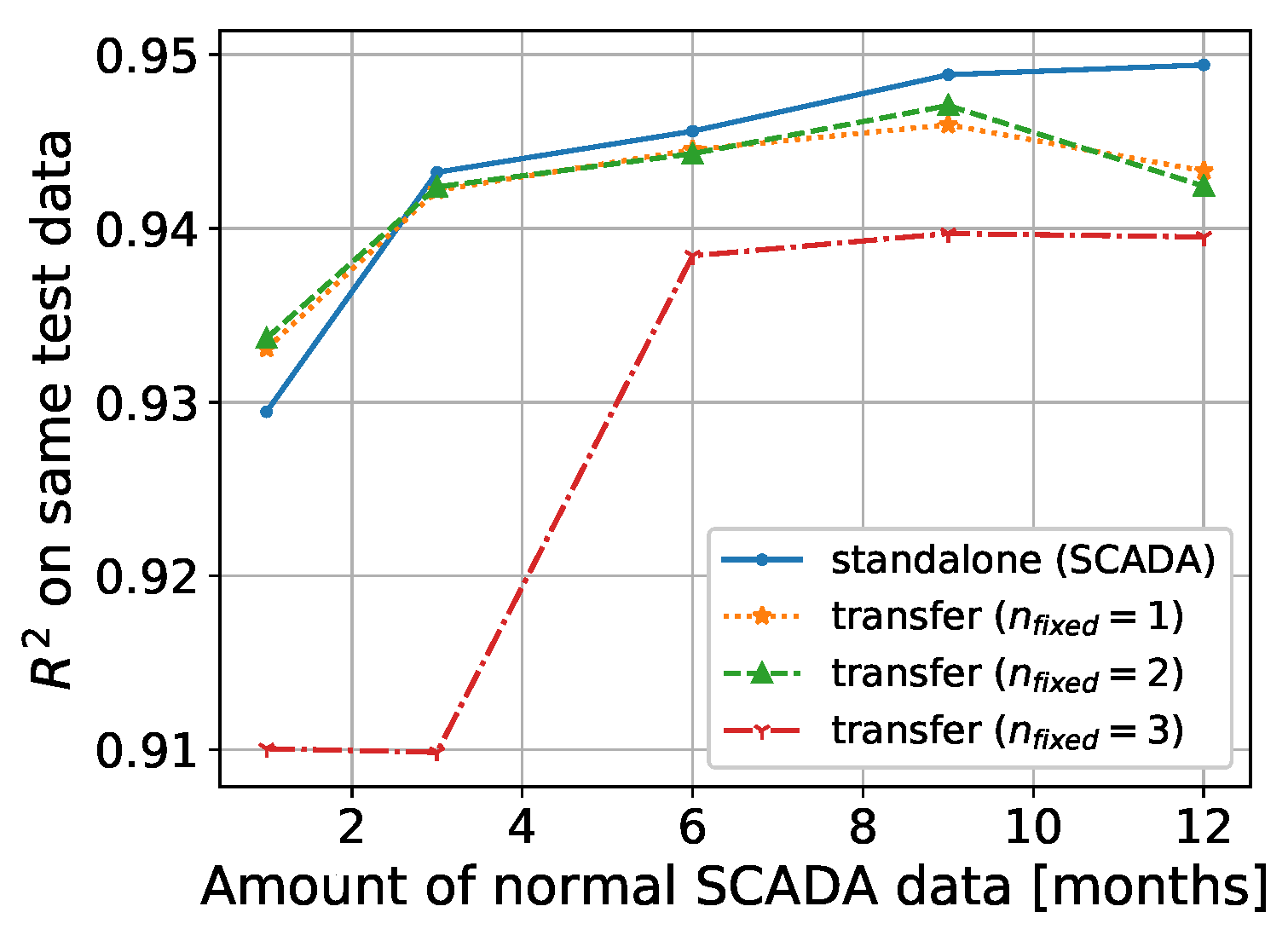
The target model is trained for five different data scales (1, 3, 6, 9 and 12 months) and four different parameter transfer scales (no parameter transfer, from one to three layers transferred from source model) resulting in 20 different model set ups. The resulting prediction accuracy of these models on the test set are presented in Figure 10. Each boxplot presents the distribution of R 2 values of the five model iterations within the five-fold crossvalidation. For the transfer learning ( 4 n f i x e d ) layers of the source model were retrained on the SCADA data with 100 epochs. The NRMSE distributions of the models are not shown since they follow a similar pattern as the R 2 values. The mean and standard deviation of the prediction accuracy of each model is shown with respect to the amount of SCADA data used for the training in Figure 11 and Figure 12 and Table 1. Finally, a comparison of the model performances tested on the same 3 months period is shown in Figure 13.

3.6. Autoencoder (Subspace Transfer)

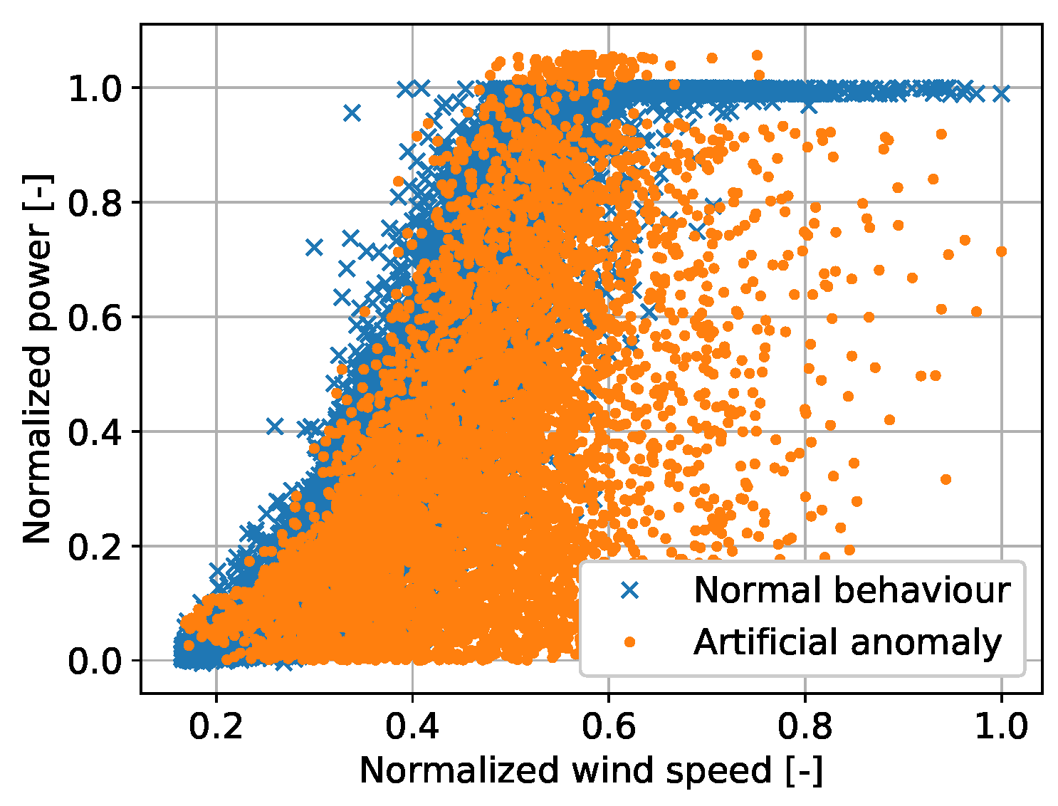
The hyperparameter tuning of the autoencoder requires more effort compared to the previous ANN since we need to make sure that autoencoder also works on detecting anomalies and does not simply reconstruct power by using the power solely. Therefore, its ability to detect anomalies on a validation data set with artificially introduced anomalies was also considered during the tuning process. An artificial validation data set was constructed based on 3 months of normal filtered SCADA data P n o r m a l , by including 43% of abnormal observations P a b n o r m a l , of which 10% represent an abnormal increase in power between 100 and 300 kW, and the remaining 90% represent a 300–500 kW increase in power (see Figure 14). These power differences were created by randomly sampling from an uniform distribution.
The fine-tuned model consists of three mirrored hidden layers with 25, 15 and 5 neurons in layer L 1 , L 2 and L 3 respectively. As a result of the hyperparameter tuning, the input was standardized and a Gaussian noise with a standard deviation of 0.1, and a noise factor of 0.5 was added. The training was conducted with the AdaDelta optimizer using a learning rate of 0.001, 600 epochs and a batch size of 400. The weights were initialized using a glorot uniform distribution, and a relu function was used as activation function for the hidden layers, and a linear function was used as activation function for the output layer.
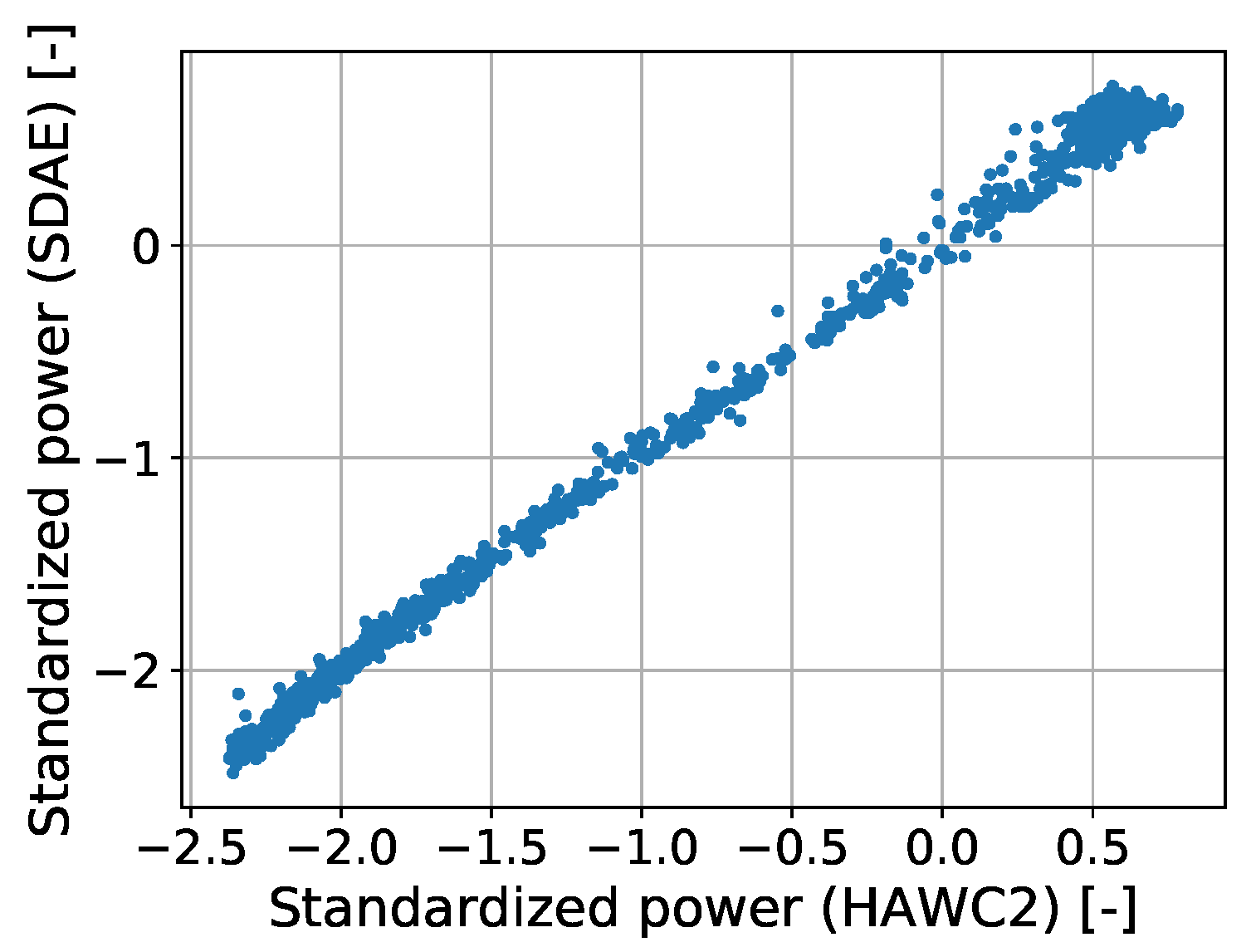
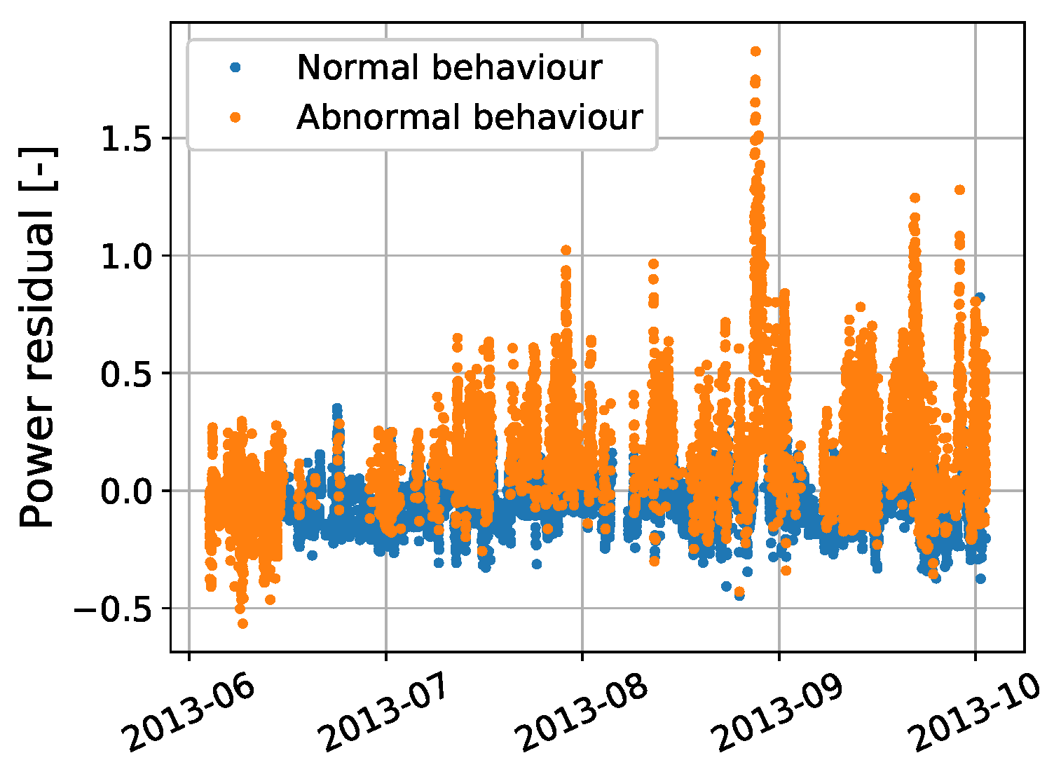
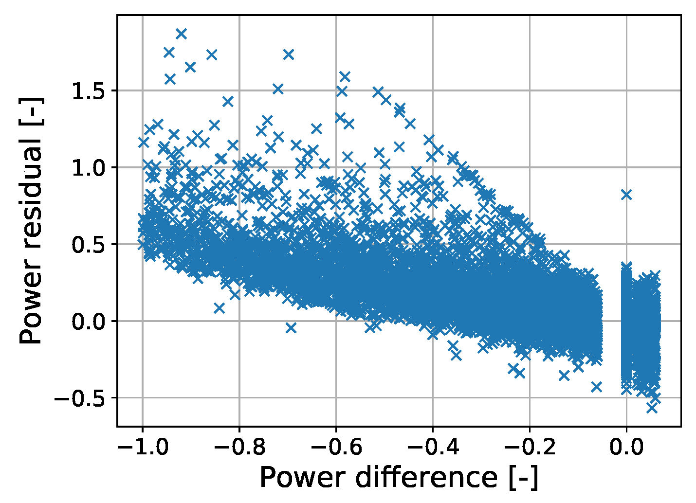
Figure 15 and Figure 16 show the prediction performance of the source model. The source model reconstructs the simulations of the test set with a R 2 value of 0.997 and NRMSE of 0.012‱. Figure 17 shows the reconstruction error of the source model when it is applied to the SCADA data with artificially introduced anomalies. In Figure 18, the reconstruction error is presented with respect to the abnormal power difference.
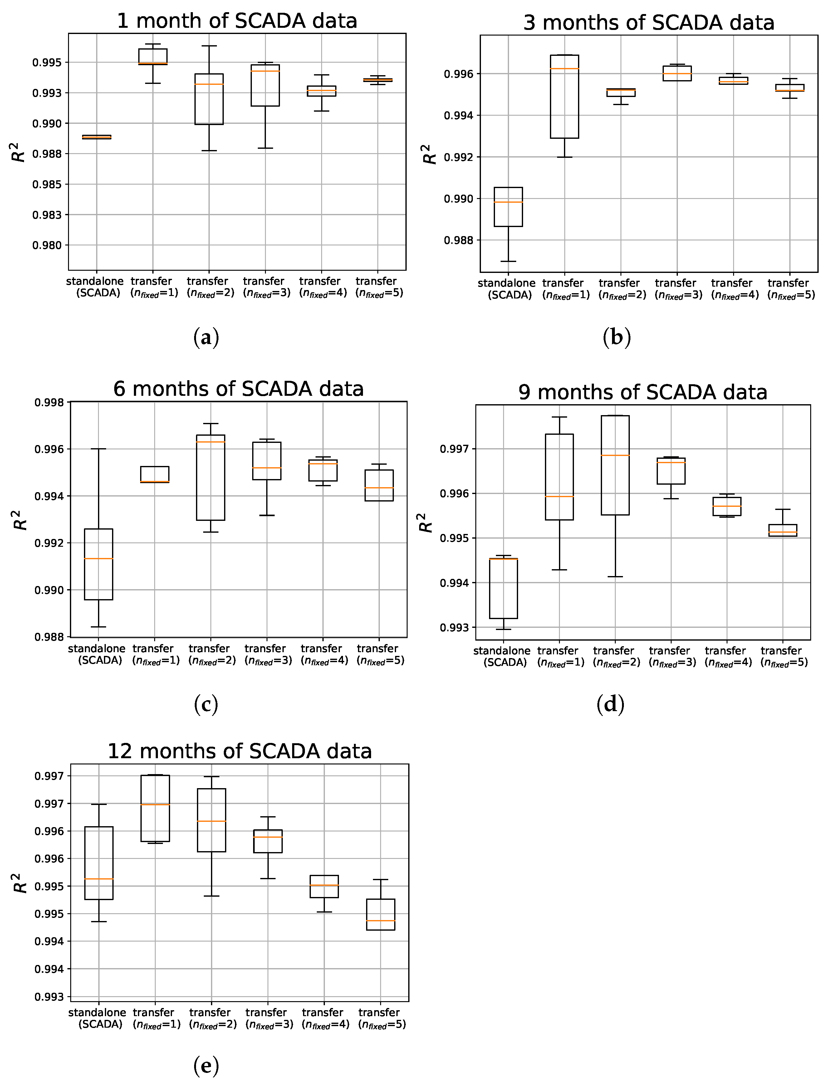
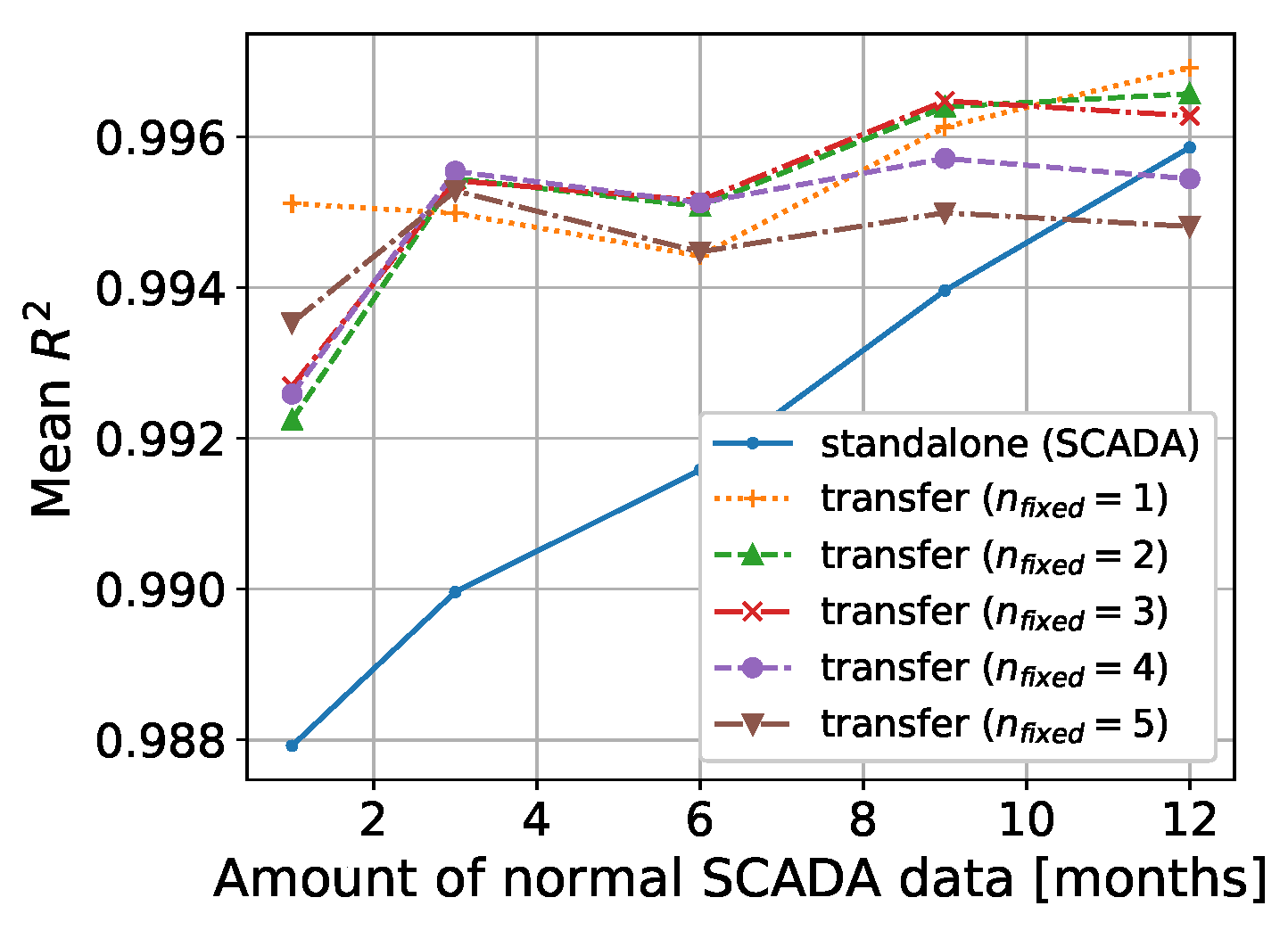
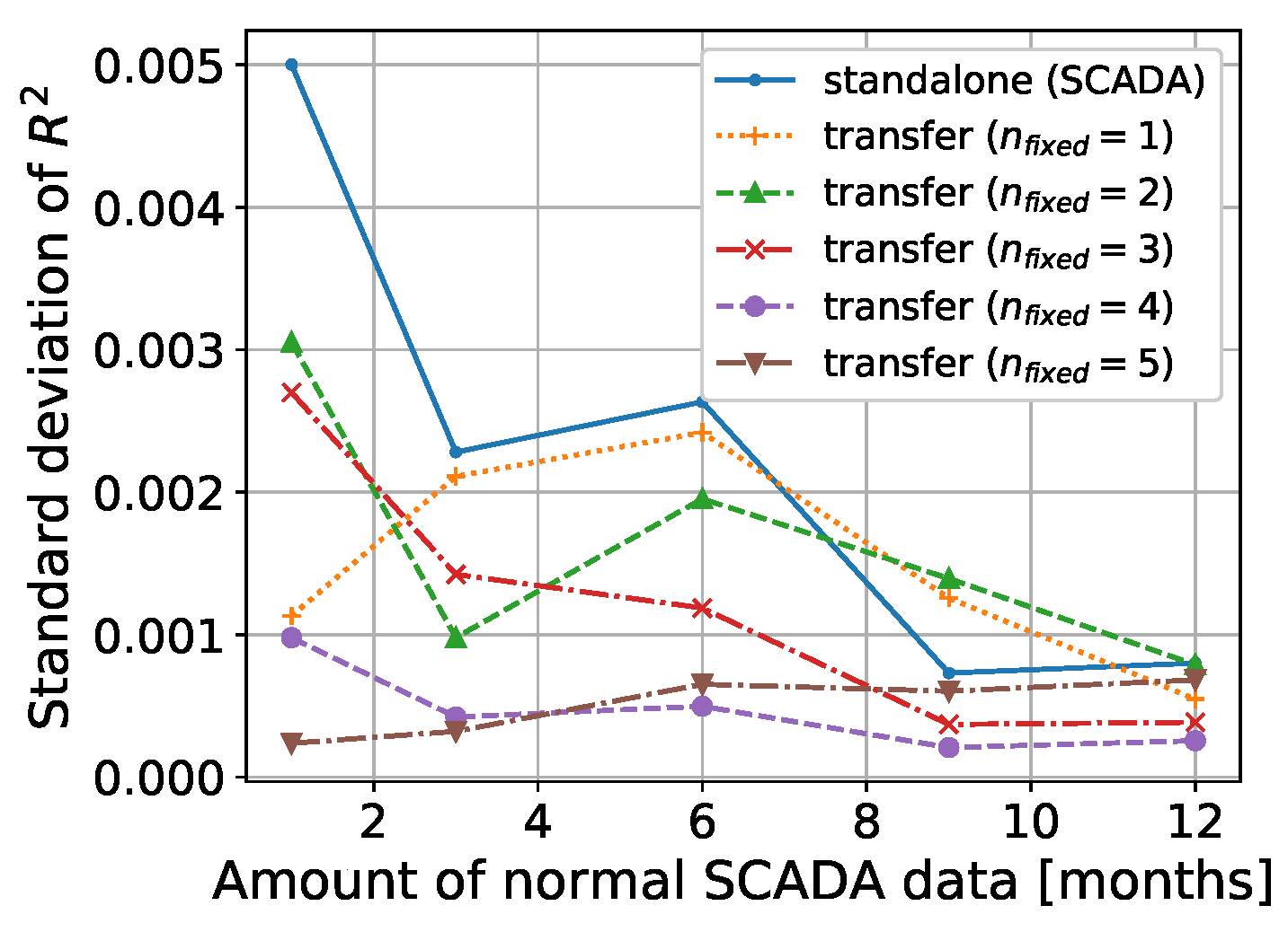
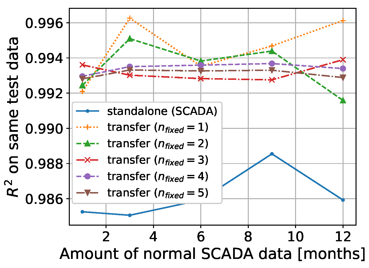
For the transfer learning, the last one and up to five layers of the source model were retrained on the SCADA data using 100 epochs. The prediction accuracy of the autoencoder on the test set is presented in Figure 19 with each boxplot presenting the distribution of R 2 values of each five-fold crossvalidation. Furthermore, the average accuracy metrics of the models are shown in Table 2. Figure 20 and Figure 21 illustrate the mean and standard deviation of the models for different amounts of SCADA data with respect to the amount of SCADA data used for the training. Similar as for the ANN, Figure 22 shows the model performances using the same 3 months test data.

3.7. Anomaly Detection

The ANN shows the largest increase in prediction performance when physics constraints are added to its training. Therefore, the comparison of the detection ability between a standalone SCADA model and physics-informed model is presented in this section for the ANN model. The results are demonstrated for the specific use case when having one month of SCADA data available, as this shows the biggest potential for augmenting the model with aeroelastic simulations. The models with the highest prediction accuracy on the training set were selected. For the transfer learning model, this means an ANN that is pretrained on simulations and recalibrated using one month of SCADA data with keeping the first two hidden layers fixed.
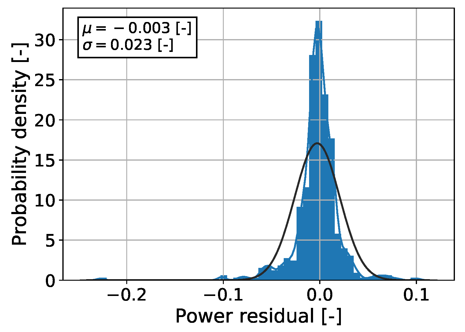
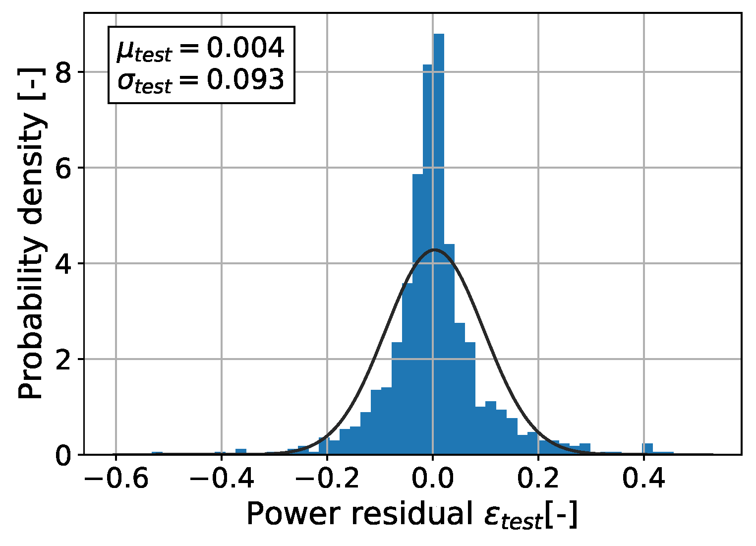
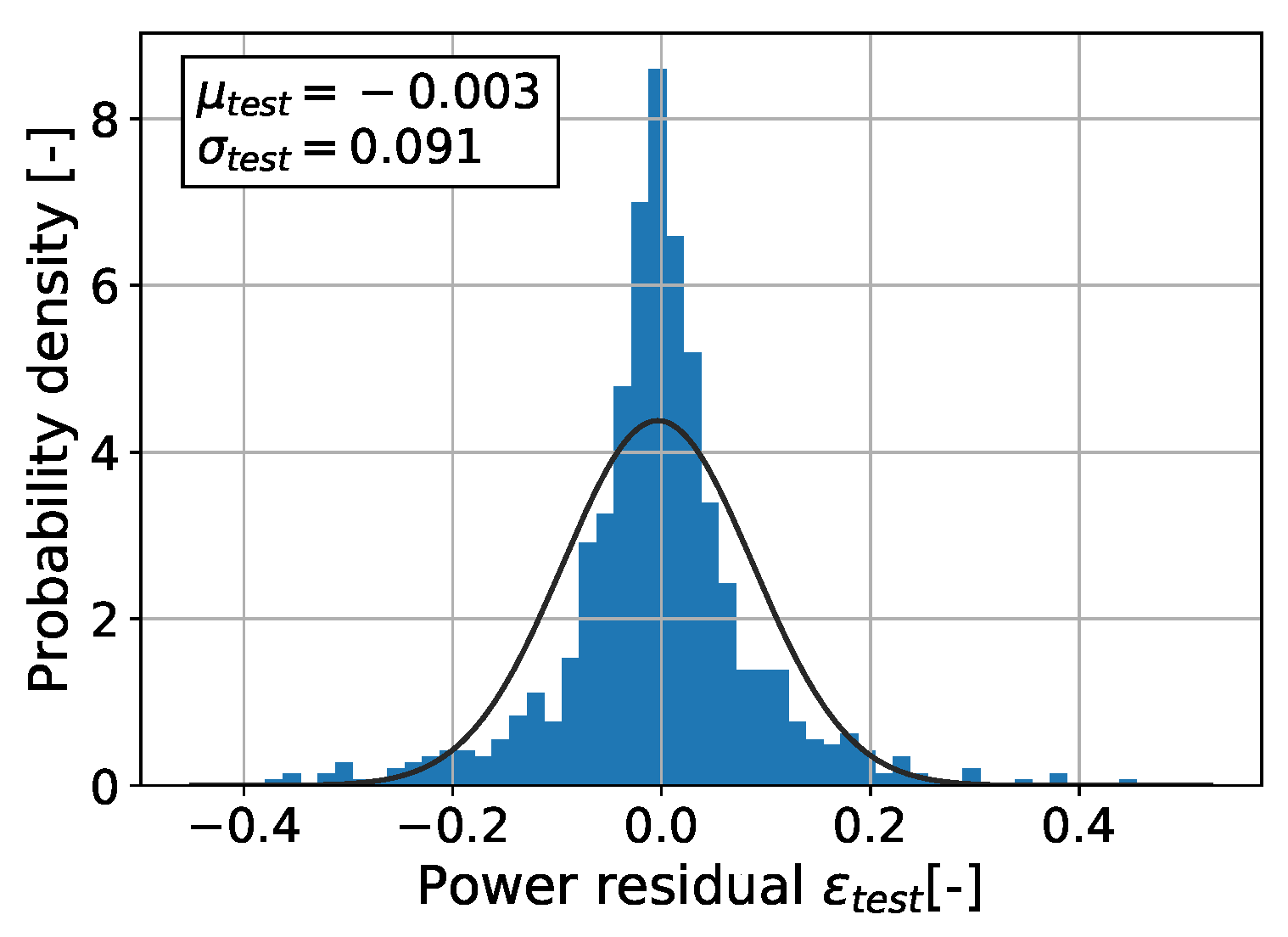
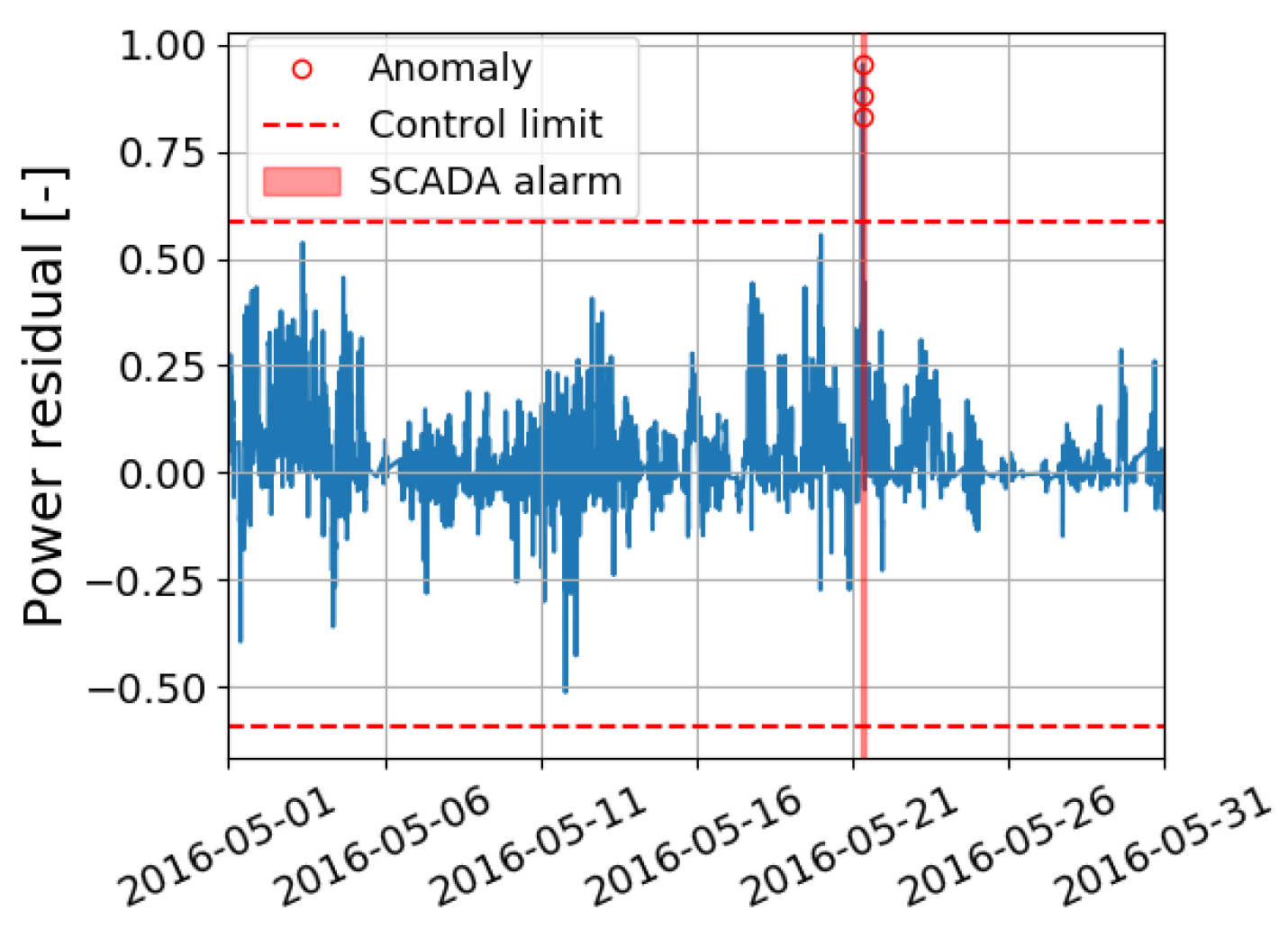
The power measurements and estimates were scaled using a min-max normalization, and the prediction residuals and corresponding control limits for each model were calculated using Equations (5) and (6). Figure 23 and Figure 24 show the distributions of the testing residuals ϵ on the normal SCADA data, including a fitted normal distribution. The selected model trained purely on SCADA data predicts the power with a R 2 value of 0.924, and the physics-informed model with a R 2 value of 0.933. Finally, Figure 25 and Figure 26 show the residuals of the model predictions on raw SCADA data for the selected period of May 2016. The time frame in which a known case of ’implausible blade angle’ was recorded by the SCADA system is marked red. The implemented monitoring system indicated several potential issues (red circles); however, the SCADA-based model without transfer learning also results in false positives. The calculated performance metrics for the precision and recall of both detection models are presented in Table 3. A precision of 100% in this case means that all observations that are classified as potential issue by the model are indeed faulty observations.

4. Discussion

The results show that the sample efficiency of a SCADA-based ANN can be significantly improved by pretraining it on a large aeroelastic simulation database. In the case when only one month of measurement data are available, the model prediction error is reduced by a NRMSE reduction of 1.64% (see Figure 11). Furthermore, the decreased standard deviation of the model accuracy for repeated model calibrations from σ ( R 2 ) = 0.02 to σ ( R 2 ) = 0.003 (see Figure 12) shows that the predictions become more robust when the suggested transfer learning method is applied. However, both in terms of the model accuracy as well as its robustness, it can be seen that the more SCADA data available for building a monitoring model, the less improvement can be achieved. The optimal learning transfer of the ANN with three hidden layers is to keep the first two layers from the source model fixed. Keeping all hidden layers fixed and only retraining the output layer on the SCADA data, on the other hand, results in a negative learning transfer, i.e., a decreased model performance compared to the standalone SCADA-based ANN. In this case the physics constraints seem to be to large for improving the target learning task of the normal power estimation. The prediction accuracy of the models compared on the same 3 months test period in Figure 10 shows slightly different results since only one fixed training period is used as compared the crossvalidation method mentioned above. However, the results confirm as well an increased accuracy when keeping up to two layers fixed and decreased performance when all hidden layers are fixed.
The model evaluation of the SDAE on the other hand shows that it already is able to accurately reconstruct the power with a R 2 value of 0.99 when only using the SCADA data for its training even for small amounts of available SCADA data (see Figure 19). The likely reason for this high accuracy is that by definition, the autoencoder uses the power signal as input to reconstruct itself. Due to this high accuracy, the application of transfer learning only improves the prediction accuracy and the model robustness on an insignificantly small scale, as it can be seen in Figure 20, Figure 21 and Figure 22. The validation of the SDAE on the data set with artificially introduced anomalies shows that it is possible to differentiate between abnormal and normal data with the help of the reconstruction error. However, a good prediction performance of the normal power does not inherently result in a better anomaly detection. The anomaly detection was only tested for the ANN-based model, since the ANN shows the largest improvements when physics constraints are added to the training.
Figure 25 and Figure 26 show that the recorded blade angle anomaly can successfully be detected by both the SCADA standalone ANN as well as the physics-informed ANN. As mentioned in Section 2, it is crucial for a good monitoring system to reduce the number of false positives. By including simulations into the model, the number of false positives could be reduced, and with it, the precision of the system improved from 50% to 100%. It should be noted that this validation study solely serves as a simple illustration to show what impact the suggested physics-informed ML approach could have on the anomaly detection ability of the monitoring system. The calculated precision and recall values, however, should be interpreted with caution since they are demonstrated only on a one month period and are strongly dependent on the threshold settings, which are defined during the model training based on the residual distributions. Furthermore, the classification of the raw SCADA observations to normal and abnormal operation is based on the limited information of the turbines system that the authors obtained from the SCADA alarms.
In general, the implications of augmenting SCADA-based monitoring models with the simulated data depends on various factors during the modeling process: Firstly, the simulation settings should be selected in order to model the turbine as representative as possible under the given environmental conditions. Here, uncertainties of the simulations might arise from the variable space definitions, environmental input selection and the wake model used [15]. Secondly, the aeroelastic model itself inhibits strengths and weaknesses in modeling the physical system of the turbine physics. One strength is its capability in modeling the rotor dynamics. Hence, adding aeroelastic simulations into SCADA-based monitoring systems can be especially beneficial for detecting anomalies related to the rotor. Another advantage of using aeroelastic simulations is that additional outputs, which are not available in the SCADA data, can be added to a multioutput model. However, this would require adjustments to the transfer learning method and is not the scope of this paper, since the authors do not have access to data for testing the results. A disadvantage of using simulations is that temperatures are not modeled in HAWC2; hence, for detecting anomalies that are detectable by rising temperatures, such as gearbox or bearing failures, the suggested procedure might not improve the monitoring system. Despite these above-described uncertainties and data limitations, the comparison of the simulations with the SCADA measurements Figure 7 shows that the simulations capture the measured behavior relatively well. A smaller rated wind speed and slightly different rotor speed curve can be noted. The reason for this deviation is that the actual industrial controller of the turbine is not available for this study. Finally, the performance of the normal behavior model is largely dependent on the filtering of the data to normal behavior as well as how an anomaly is defined, i.e., on the threshold setting.

5. Conclusions and Future Work

This paper introduces a novel approach to include physics into data-driven normal behavior monitoring models for detecting turbine anomalies by means of transfer learning. For this purpose, a normal behavior model was pretrained on a large simulation database and recalibrated on the available SCADA data via transfer learning. For two methods, an ANN and an autencoder, it was investigated under which conditions it can be helpful to include simulations into SCADA-based monitoring systems. The results show that when only one month of SCADA data is available, both the model accuracy as well as the model robustness of an ANN is significantly improved by adding physics constraints from a pretrained model. The model prediction error NRMSE is reduced by 1.64%, while the standard deviation of the model accuracy for repeated model calibrations is reduced from σ ( R 2 ) = 0.02 to σ ( R 2 ) = 0.003. The optimal amount of knowledge transfer in this set up is to keep two of the three hidden layers from the pretrained model fixed and recalibrate the third hidden and the output layer on the SCADA data. Keeping all hidden layers fixed would result in a negative learning transfer. As the autoencoder reconstructs the power from itself, it is already able to accurately model the normal behavior power. Therefore, including simulations into the model does not improve its prediction performance and robustness significantly. The validation of the physics-informed ANN on one month of raw SCADA data shows that it is able to successfully detect the recorded blade angle anomaly with an precision improvement from 50% to 100%, i.e., less false positives compared to its purely SCADA data-based counterpart.
In order to analyze the full implications of augmenting simulations into the data-driven model, future work should focus on a full validation study including further different anomaly cases as well as to test whether the autoencoder has improved its detection ability. Furthermore, since building an accurate aeroelastic model of a specific turbine requires the effort and expertise of the system, it would be interesting to investigate how the level of accuracy of the aeroelastic model influences the final monitoring performance. Finally, for detecting anomalies, a constant residual distribution with respect to the wind speed is assumed for calculating the normal threshold. However, more advanced techniques for calculating confidence intervals that take into account the heteroscedasticity of the residuals and for interpreting the residual patterns can be used. In the end, for the continuation of the research, the effectiveness of the proposed method can be compared against other data enrichment techniques which are based only on measured data.

Author Contributions

Conceptualization, L.S.; methodology, L.S.; software, L.S.; validation, L.S.; formal analysis, L.S.; investigation, L.S.; data curation, L.S.; writing—original draft preparation, L.S.; writing—review and editing, L.S., N.K.D., D.R.V. and J.A.S.; visualization, L.S.; supervision, N.K.D., D.R.V. and J.A.S. All authors have read and agreed to the published version of the manuscript.

Funding

This research received no external funding.

Institutional Review Board Statement

Not applicable.

Informed Consent Statement

Not applicable.

Data Availability Statement

The HAWC2 simulation data set used in this study can be found at https://doi.org/10.11583/DTU.12245978 (accessed on 10 January 2022).

Conflicts of Interest

The authors declare no conflict of interest.

References

  1. WWEA. Worldwide Wind Capacity Reaches 744 Gigawatts. Germany. 2021. Available online: https://wwindea.org/worldwide-wind-capacity-reaches-744-gigawatts/ (accessed on 10 January 2021).
  2. Stetco, A.; Dinmohammadi, F.; Zhao, X.; Robu, V.; Flynn, D.; Barnes, M.; Keane, J.; Nenadic, G. Machine learning methods for wind turbine condition monitoring: A review. Renew. Energy 2019, 133, 620–635. [Google Scholar] [CrossRef]
  3. Schlechtingen, M.; Santos, I.F.; Achiche, S. Wind turbine condition monitoring based on SCADA data using normal behavior models. Part 1: System description. Appl. Soft Comput. 2013, 13, 259–270. [Google Scholar] [CrossRef]
  4. Tautz-Weinert, J.; Watson, S.J. Using SCADA data for wind turbine condition monitoring—A review. IET Renew. Power Gener. 2016, 11, 382–394. [Google Scholar] [CrossRef] [Green Version]
  5. Zaher, A.; McArthur, S.; Infield, D.; Patel, Y. Online wind turbine fault detection through automated SCADA data analysis. Wind. Energy Int. J. Prog. Appl. Wind. Power Convers. Technol. 2009, 12, 574–593. [Google Scholar] [CrossRef]
  6. Von Rueden, L.; Mayer, S.; Garcke, J.; Bauckhage, C.; Schuecker, J. Informed machine learning–towards a taxonomy of explicit integration of knowledge into machine learning. Learning 2019, 18, 19–20. [Google Scholar]
  7. Garcia, M.C.; Sanz-Bobi, M.A.; Del Pico, J. SIMAP: Intelligent System for Predictive Maintenance: Application to the health condition monitoring of a windturbine gearbox. Comput. Ind. 2006, 57, 552–568. [Google Scholar] [CrossRef]
  8. Cross, P.; Ma, X. Model-based and fuzzy logic approaches to condition monitoring of operational wind turbines. Int. J. Autom. Comput. 2015, 12, 25–34. [Google Scholar] [CrossRef] [Green Version]
  9. Tipireddy, R.; Tartakovsky, A. Physics-informed Machine Learning Method for Forecasting and Uncertainty Quantification of Partially Observed and Unobserved States in Power Grids. arXiv 2018, arXiv:1806.10990. [Google Scholar]
  10. Nascimento, R.G.; Viana, F.A. Fleet prognosis with physics-informed recurrent neural networks. arXiv 2019, arXiv:1901.05512. [Google Scholar]
  11. Yucesan, Y.A.; Viana, F.A. Wind Turbine Main Bearing Fatigue Life Estimation with Physics-informed Neural Networks. In Proceedings of the Annual Conference of the PHM Society, Scottsdale, AZ, USA, 23 September 2019; Volume 11. [Google Scholar]
  12. Pan, S.J.; Yang, Q. A survey on transfer learning. IEEE Trans. Knowl. Data Eng. 2009, 22, 1345–1359. [Google Scholar] [CrossRef]
  13. Zhuang, F.; Qi, Z.; Duan, K.; Xi, D.; Zhu, Y.; Zhu, H.; Xiong, H.; He, Q. A comprehensive survey on transfer learning. Proc. IEEE 2020, 109, 43–76. [Google Scholar] [CrossRef]
  14. Dimitrov, N. Surrogate models for parameterized representation of wake-induced loads in wind farms. Wind. Energy 2019, 22, 1371–1389. [Google Scholar] [CrossRef]
  15. Schröder, L.; Dimitrov, N.K.; Verelst, D.R. A surrogate model approach for associating wind farm load variations with turbine failures. Wind. Energy Sci. 2020, 5, 1007–1022. [Google Scholar] [CrossRef]
  16. Larsen, T.J.; Hansen, A.M. How 2 HAWC2, the user’s manual. Target 2019, 2, 2. [Google Scholar]
  17. Madsen, H.A.; Larsen, T.J.; Pirrung, G.R.; Li, A.; Zahle, F. Implementation of the blade element momentum model on a polar grid and its aeroelastic load impact. Wind. Energy Sci. 2020, 5, 1–27. [Google Scholar] [CrossRef] [Green Version]
  18. Mann, J. Wind field simulation. Probabilistic Eng. Mech. 1998, 13, 269–282. [Google Scholar] [CrossRef]
  19. Larsen, G.C.; Madsen, H.A.; Thomsen, K.; Larsen, T.J. Wake meandering: A pragmatic approach. Wind. Energy Int. J. Prog. Appl. Wind. Power Convers. Technol. 2008, 11, 377–395. [Google Scholar] [CrossRef]
  20. Schlechtingen, M.; Santos, I.F. Comparative analysis of neural network and regression based condition monitoring approaches for wind turbine fault detection. Mech. Syst. Signal Process. 2011, 25, 1849–1875. [Google Scholar] [CrossRef] [Green Version]
  21. Schröder, L.; Dimitrov, N.K.; Verelst, D.R.; Sørensen, J.A. Wind turbine site-specific load estimation using artificial neural networks calibrated by means of high-fidelity load simulations. J. Phys. Conf. Ser. 2018, 1037, 062027. [Google Scholar] [CrossRef]
  22. Renström, N.; Bangalore, P.; Highcock, E. System-wide anomaly detection in wind turbines using deep autoencoders. Renew. Energy 2020, 157, 647–659. [Google Scholar] [CrossRef]
  23. Chen, J.; Li, J.; Chen, W.; Wang, Y.; Jiang, T. Anomaly detection for wind turbines based on the reconstruction of condition parameters using stacked denoising autoencoders. Renew. Energy 2020, 147, 1469–1480. [Google Scholar] [CrossRef]
  24. Kusiak, A.; Zheng, H.; Song, Z. Models for monitoring wind farm power. Renew. Energy 2009, 34, 583–590. [Google Scholar] [CrossRef]
  25. Reder, M.D.; Gonzalez, E.; Melero, J.J. Wind turbine failures-tackling current problems in failure data analysis. J. Phys. Conf. Ser. 2016, 753, 072027. [Google Scholar] [CrossRef]
  26. Optis, M.; Perr-Sauer, J.; Philips, C.; Craig, A.E.; Lee, J.C.; Kemper, T.; Sheng, S.; Simley, E.; Williams, L.; Lunacek, M.; et al. OpenOA: An Open-Source Code Base for Operational Analysis of Wind Power Plants. Wind Energ. Sci. 2019, 10, 1–14. [Google Scholar] [CrossRef]
  27. Vorpahl, F.; Popko, W.; Kaufer, D. Description of a Basic Model of the “UpWind Reference Jacket” for Code Comparison in the OC4 Project under IEA Wind Annex XXX; Fraunhofer Institute for Wind Energy and Energy System Technology (IWES): Bremerhaven, Germany, 2011. [Google Scholar]
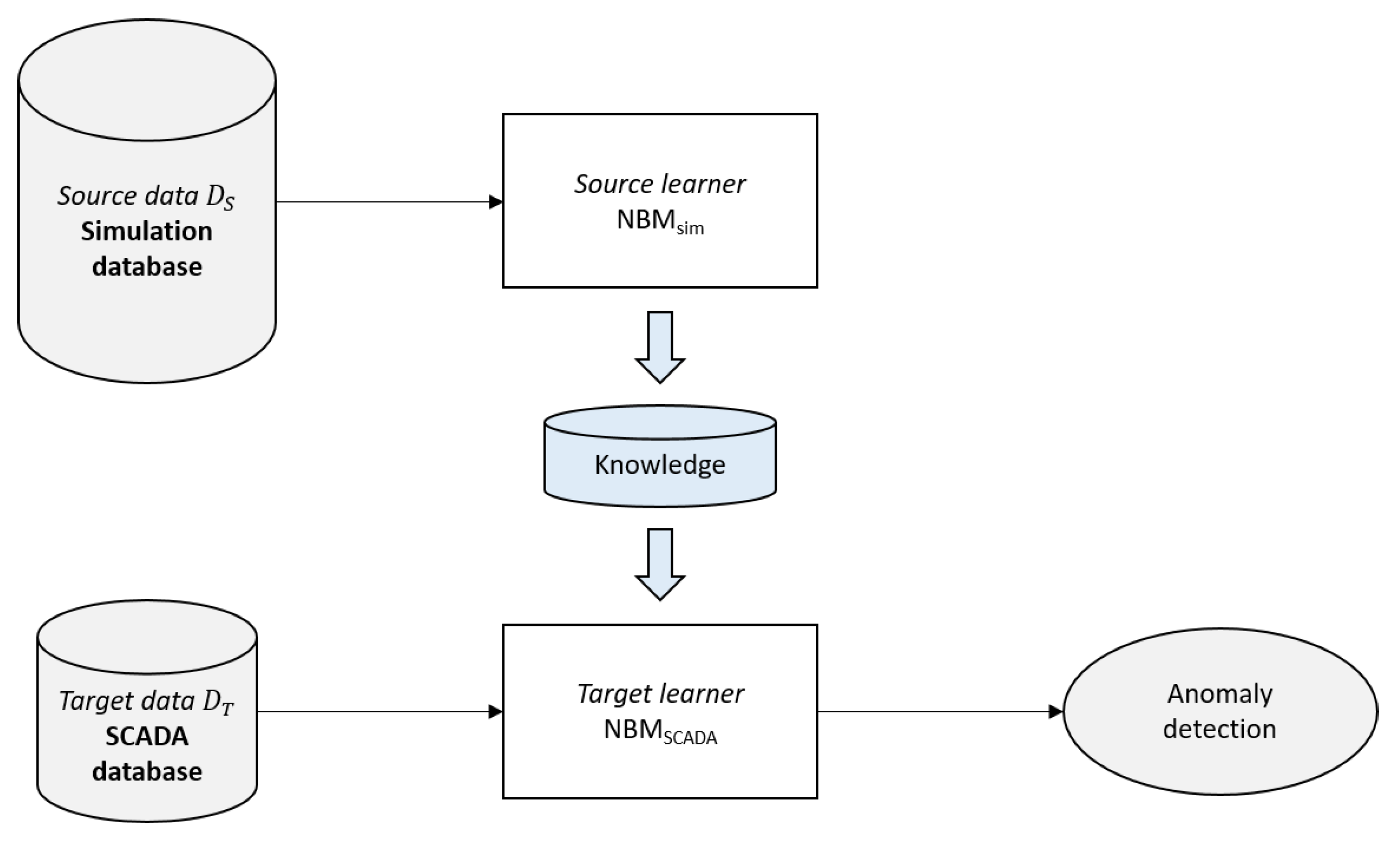
Figure 1. Schematic illustration of knowledge transfer for monitoring wind turbines using simulations and measured SCADA data.
Energies 15 00558 g001
Figure 2. Process of aero-servo-hydro-elastic simulations using sampled input variables. The figure is taken from [15] which is distributed under CC BY 4.0 License. Details of the license are available at https://creativecommons.org/licenses/by/4.0/ (8 July 2021).
Energies 15 00558 g002
Figure 3. Schematic illustration of ANN architecture with parameter transfer. Parameters from the first two layers are fixed (red), while last two layers are retrained on the target data (green).
Energies 15 00558 g003
Figure 4. Schematic illustration of architecture of an autoencoder with subspace transfer. Parameters from the first two layers are fixed (red), while last two layers are retrained on the target data (green).
Energies 15 00558 g004
Figure 5. Schematic illustration of anomaly detection. Reproduced from [4] which is distributed under CC BY-NC-ND 4.0 Licence. Details of the license are available at https://creativecommons.org/licenses/by-nc-nd/4.0/ 8 July 2021.
Energies 15 00558 g005
Figure 6. Power curve (a) and time series of power, wind speed, pitch angle and yaw angle (b) from SCADA measurements for a time period where a problem with blade angle has occurred.
Energies 15 00558 g006
Figure 7. Comparison of measured and simulated data used for building a normal behavior model including (a) power, (b) pitch angle and (c) rotor speed with respect to the wind speed.
Energies 15 00558 g007
Figure 8. Normalized power estimated by ANN on test set of source data with respect to normalized power simulations.
Energies 15 00558 g008
Figure 9. Normalized power estimated by ANNon test setwith respect to normalized power simulations.
Energies 15 00558 g009
Figure 10. ANN target model performance on different amounts of normal SCADA data and knowledge transfers. Each boxplot represents the R 2 distribution of the models trained within the five-fold crossvalidation. The target models are trained using 1 month (a), 3 months (b), 6 months (c), 9 months (d), and 12 months (e) of normal SCADA data.
Energies 15 00558 g010
Figure 11. Average R 2 value for ANN for different amounts of training data and knowledge transfers.
Energies 15 00558 g011
Figure 12. Standard deviation of R 2 value for ANN for different amounts of training data and knowledge transfers.
Energies 15 00558 g012
Figure 13. R 2 value for ANN for different amounts of training data and knowledge transfers tested on same 3 months test data.
Energies 15 00558 g013
Figure 14. Data set with artificially introduced anomalies for hyperparameter tuning of autoencoder model.
Energies 15 00558 g014
Figure 15. Standardized power estimated by SDAE on test set with respect to normalized power simulations.
Energies 15 00558 g015
Figure 16. Normalized power estimated by SDAE on test set with respect to normalized power simulations.
Energies 15 00558 g016
Figure 17. Reconstruction error of SDAE on normal operating data (blue) and artificially introduced anomalies (orange).
Energies 15 00558 g017
Figure 18. Reconstruction error of SDAE with respect to normalized power deviation P a b n o r m a l P n o r m a l .
Energies 15 00558 g018
Figure 19. Autoencoder target model performance on different amounts of normal SCADA data and knowledge transfers. Each boxplot represents the R 2 distribution of the models trained within the five-fold crossvalidation. The target models are trained using 1 month (a), 3 months (b), 6 months (c), 9 months (d) and 12 months (e) of normal SCADA data.
Energies 15 00558 g019
Figure 20. Average R 2 value for SDAE for different amounts of training data and knowledge transfers.
Energies 15 00558 g020
Figure 21. Standard deviation of R 2 value for SDAE for different amounts of training data and knowledge transfers.
Energies 15 00558 g021
Figure 22. R 2 value for SDAE for different amounts of training data and knowledge transfers tested on same 3 months test data.
Energies 15 00558 g022
Figure 23. Probability density function of testing residuals including normal distribution fit for standalone SCADA model.
Energies 15 00558 g023
Figure 24. Probability density function of testing residuals including normal distribution fit for transfer learning model.
Energies 15 00558 g024
Figure 25. Power residuals of standalone SCADA model applied to raw SCADA data of May 2016.
Energies 15 00558 g025
Figure 26. Power residuals of transfer learning model applied to raw SCADA data of May 2016.
Energies 15 00558 g026
Table 1. Prediction performance of ANN for different amounts of training data and knowledge transfers.
Mean R 2 Mean NRMSE (%)
136912136912
SCADA0.9010.9580.9560.9580.95911.067.587.447.577.45
n f i x e d = 10.9270.9580.9560.9580.9589.537.567.477.617.51
n f i x e d = 20.9290.9580.9570.9580.9589.427.537.407.557.50
n f i x e d = 30.9130.9500.9510.9540.95310.438.257.897.957.96
Table 2. Prediction performance of SDAE for different amounts of training data and knowledge transfers.
R 2 NRMSE (‱)
136912136912
standalone0.9880.9900.9920.9940.9960.020.020.020.020.01
n f i x e d = 10.9950.9950.9940.9960.9970.020.020.020.010.01
n f i x e d = 20.9920.9950.9950.9960.9970.020.020.020.010.01
n f i x e d = 30.9930.9950.9950.9970.9960.020.020.020.010.01
n f i x e d = 40.9930.9960.9950.9960.9950.020.020.020.020.02
n f i x e d = 50.9940.9950.9950.9950.9950.020.020.020.020.02
Table 3. Detection performance of standalone SCADA-based ANN and transfer learning ANN on one month of raw SCADA data.
SCADA Stanrdalone ANNTransfer Learning ANN
Precision50%100%
Recall100%100%
Publisher’s Note: MDPI stays neutral with regard to jurisdictional claims in published maps and institutional affiliations.