
A Stochastic Petri Net Model for O&M Planning of Floating Offshore Wind Turbines


1
Department of Energy and Power, Cranfield University, College Road, Bedfordshire MK43 0AL, UK
2
Mechanical Engineering Group, School of Engineering, University of Kent, Canterbury CT2 7NT, UK
3
The Bartlett Centre for Advanced Spatial Analysis (CASA), University College London (UCL), Gower Street, London WC1E 6BTL, UK
*
Author to whom correspondence should be addressed.
Energies 2021, 14(4), 1134; https://doi.org/10.3390/en14041134
Submission received: 29 January 2021
/
Revised: 12 February 2021
/
Accepted: 18 February 2021
/
Published: 20 February 2021
(This article belongs to the Special Issue Lifetime Extension of Wind Turbines and Wind Farms)
Abstract
:With increasing deployment of offshore wind farms further from shore and in deeper waters, the efficient and effective planning of operation and maintenance (O&M) activities has received considerable attention from wind energy developers and operators in recent years. The O&M planning of offshore wind farms is a complicated task, as it depends on many factors such as asset degradation rates, availability of resources required to perform maintenance tasks (e.g., transport vessels, service crew, spare parts, and special tools) as well as the uncertainties associated with weather and climate variability. A brief review of the literature shows that a lot of research has been conducted on optimizing the O&M schedules for fixed-bottom offshore wind turbines; however, the literature for O&M planning of floating wind farms is too limited. This paper presents a stochastic Petri network (SPN) model for O&M planning of floating offshore wind turbines (FOWTs) and their support structure components, including floating platform, moorings and anchoring system. The proposed model incorporates all interrelationships between different factors influencing O&M planning of FOWTs, including deterioration and renewal process of components within the system. Relevant data such as failure rate, mean-time-to-failure (MTTF), degradation rate, etc. are collected from the literature as well as wind energy industry databases, and then the model is tested on an NREL 5 MW reference wind turbine system mounted on an OC3-Hywind spar buoy floating platform. The results indicate that our proposed model can significantly contribute to the reduction of O&M costs in the floating offshore wind sector.
1. Introduction
The wind energy industry is expanding its frontiers throughout the world, and wind power is gradually taking over the market from fossil fuels. According to statistics from WindEurope, the total installed capacity of wind power in the European Union (EU) had reached 205 gigawatts (GW) by the end of 2019. This capacity generated 417 terawatt hours (TWh) of electricity, covering around 15% of the EU’s electricity consumption in 2019 [1]. The European Commission (EC) has recognized wind energy development, in particular offshore wind power, as one of the strategic priorities for a low-carbon future [2,3].
Offshore wind is the future of wind energy in the UK, and the government has recently set out commitments to ensure that offshore wind will power every home in the country by 2030. This boosts the government’s previous offshore wind target from 30 GW to 40 GW [4]. According to the Crown Estate’s report [5], the UK currently has the largest operational capacity of offshore wind in Europe, representing 45% of the total installed capacity. This was achieved by installing more than 1764 MW offshore wind power by the UK (out of a total 3627 MW in Europe) in 2019 [6]. Although the growth in capacity naturally leads to a reduction in the levelized cost of electricity (LCOE) from offshore wind, it drastically increases the operating expenditure (OPEX) for wind farms [7].
With the increasing number of offshore wind installations and due to limited space available near the coast in shallow waters, there is now a crucial need to move to deeper waters where wind speeds tend to be higher and more consistent [8]. Despite some benefits, the deepwater wind farms have to deal with a greater scale of challenges than shallow-water wind farms, such as the design constraints of fixed-bottom structures, a wide variation of weather conditions, and the need to hire expensive machinery or access equipment for maintenance [9]. To overcome some of these challenges, floating offshore wind turbines (FOWTs) are becoming an economically attractive option for wind energy projects in water depths greater than 60 m. FOWTs are not rigidly fixed to the seabed and thus their location is not limited to shallow waters anymore and they can cope with strong currents and severe wave conditions.
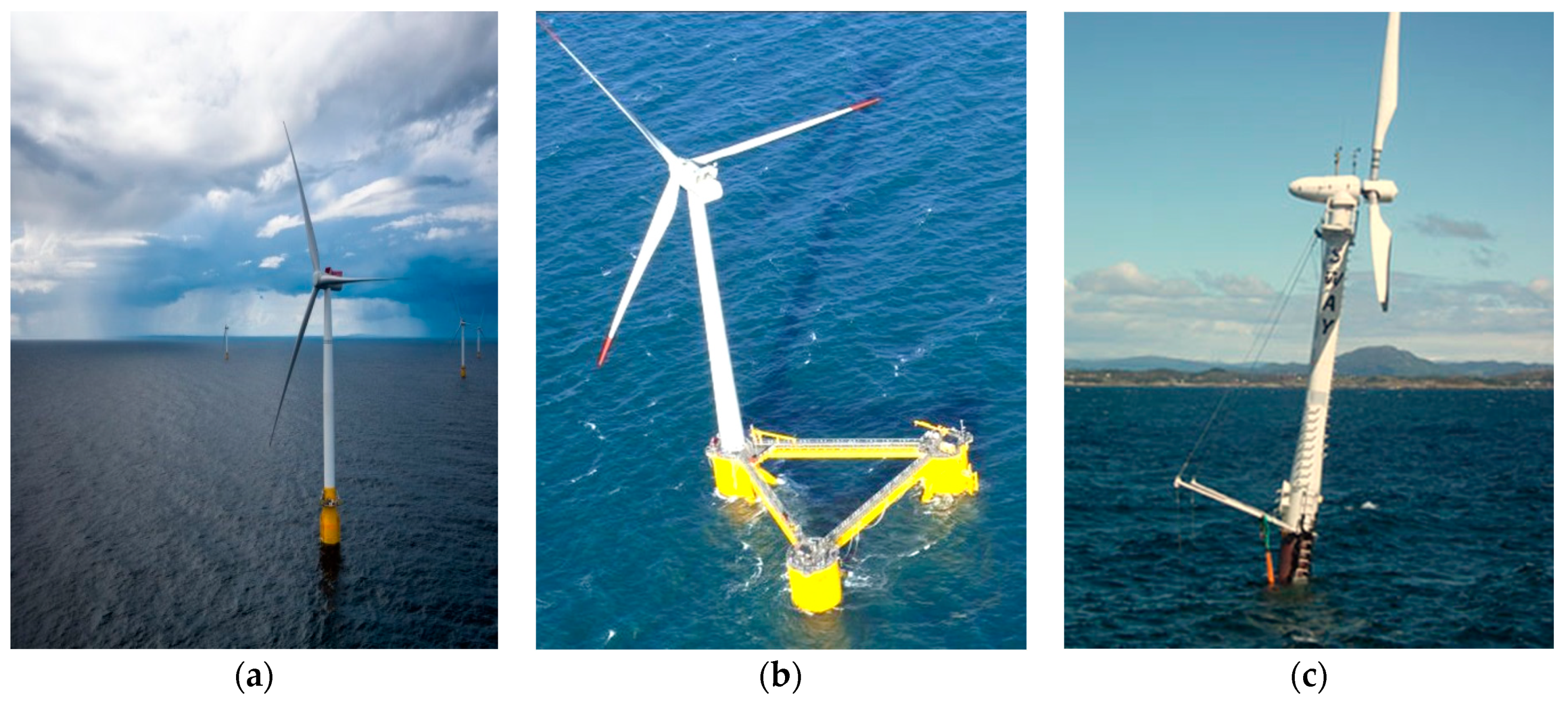
On the global scale, Europe has been at the forefront of floating wind energy development [10]. Several floating wind technologies have been developed in recent years, and the industry has been making good progress thus far. The industry’s research and development programs have mainly focused on improving the wind farms layout as well as designing floating foundations to optimise deepwater wind energy production. The floating offshore wind concepts of Hywind, WindFloat and SWAY, which are shown in Figure 1, are among the most popular technologies being tested and deployed in real-world settings [11]. Some other examples of floating wind concepts include: Blue H, WindSea, Nova, Vertax and Vertiwind [12]. There have been some research studies and pilot programs to test these concepts in controlled offshore environments. These research studies have aimed at optimising the materials properties and maintenance processes required for improved floating offshore wind farm energy generation.
Floating wind energy will be necessary for the UK to meet net-zero emissions by 2050. In addition, it can create 17,000 jobs and generate £33.6 billion for the UK economy [16]. Recently, the government has set a target of 1 GW floating wind energy capacity by 2030, which is nearly 15 times the current operational capacity worldwide. There are boundless opportunities to deploy floating wind technologies off the coast of Scotland and Wales. Hywind Scotland is the world’s first commercial floating offshore wind farm located 25 km off the coast of Peterhead in Aberdeenshire. The wind farm comprises six 5 MW floating wind turbines which will produce enough electricity to power 20,000 homes [13]. The Kincardine project is the largest floating offshore wind farm in the world by nameplate capacity which is under construction about 15 km off the coast of Aberdeen at water depths ranging from 60 to 80 m. The wind farm comprises one 2 MW and five 9.525 MW Vestas wind turbines which are being installed on triangular-shaped semi-submersible foundations [17].
In order to ensure the continued integrity and availability of FOWTs, an efficient and effective planning of operation and maintenance (O&M) activities throughout the wind farm’s life is required. Maintenance strategies aim to reduce the occurrence of failure in wind turbine assets while maximizing energy generation. The most common maintenance strategies that are adopted in the wind energy sector include: corrective, preventive, and condition-based [18]. The corrective maintenance (CM) is a type of maintenance carried out after a component has failed. The preventive maintenance (PM), also known as time-based or periodic maintenance, is carried out at predetermined time intervals to minimize the probability of unexpected breakdowns. The condition-based maintenance (CBM) is carried out based on asset health condition obtained from routine or continuous monitoring. The process of CBM involves monitoring the system to determine its operating status, predicting anomalies, and developing an appropriate maintenance plan to avoid functional failures. A CBM plan provides more cost-effective schedules for maintenance tasks than PM, as it is a more suitable method for analyzing the gradual degradation process in wind turbine systems, especially in harsh offshore environments [19].
The high cost of O&M is a major area of concern to wind energy developers and operators. Depending on the wind farm characteristics, such as the number and power rating of wind turbines, distance to shore, weather and sea state, etc. there will be different cost implications [20]. Improvements in the O&M planning of offshore wind farms could lead to considerable reduction in costs. According to the Carbon Trust [10], the O&M planning is known as one of the technical barriers for floating offshore wind farms in deep waters and harsh weather conditions. Therefore, there is a need for innovations in methods and practice that improve O&M planning of floating offshore wind farms to increase availability and safety and lower O&M expenditure. An example of innovation campaigns in the wind energy sector is the Offshore Wind Innovation Hub (https://offshorewindinnovationhub.com/ (accessed on 21 December 2020), which was set up to coordinate innovation and technology development in wind energy businesses, with a focus on offshore wind energy cost reduction.
The O&M planning of floating offshore wind farms is a very complicated task due to the diversity of components such as wind turbine parts, foundation platform, mooring cables, anchors, etc., existence of different degradation processes with unknown rates, sparsity of failure data, uncertainty of weather variability, and unpredictability of demand for spare parts and maintenance vessels. A brief review of the literature shows that very few research works have been conducted on optimizing the O&M procedures for floating offshore wind farms. To overcome this research gap, this paper proposes a stochastic Petri network (SPN) model for O&M planning of FOWT systems and their associated support structure components, including floating platform, catenary mooring lines and anchoring system. The proposed model incorporates all interrelationships between different factors influencing O&M planning of FOWTs, including deterioration and the renewal process of components within the system. Relevant data such as failure rate, mean-time-to-failure (MTTF), degradation rate, etc. are collected from the literature as well as wind energy industry databases, and then the model is tested on an NREL 5 MW reference wind turbine system with a spar-type substructure and catenary mooring lines.
The organization of the rest of this paper is as follows. Section 2 reviews the O&M planning techniques and tools adopted in the offshore wind industry, in particular for FOWTs. Section 3 presents the SPN model for O&M planning of floating offshore wind farms. Section 4 presents the case study results and discusses the findings. Finally, the paper is concluded and a few ideas for future research are proposed in Section 5.
2. Operation and Maintenance (O&M) Planning for Floating Offshore Wind Farms
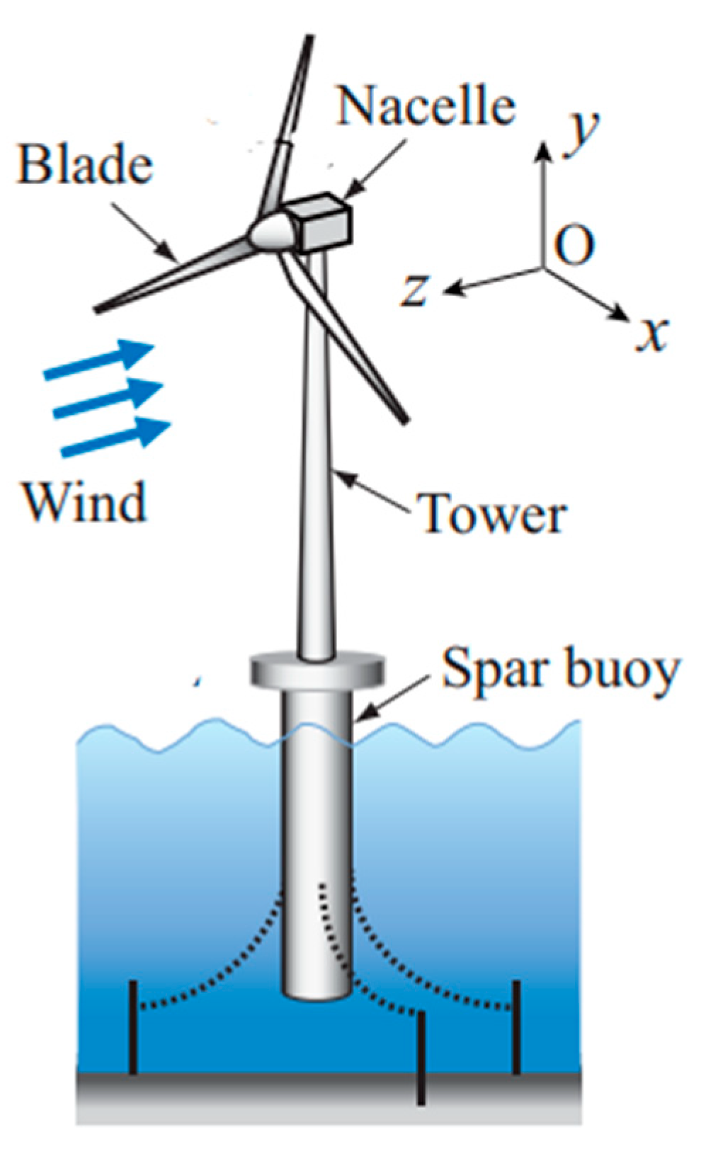
The O&M planning of floating offshore wind farms is significantly different than that of onshore wind farms or even bottom-fixed wind turbines in shallow water. This difference in O&M planning is mainly related to differences in the type of support structures (monopiles, gravity-based structures, tripods and jackets are types of foundation for bottom-fixed wind turbines, whereas the popular concepts for floating foundations are spar-buoy, semi-submersible and tension-leg platform); the presence of additional components (such as mooring lines and anchors); uncertainties associated with the components’ lifetime due to variations in loading and environmental conditions, etc. Figure 2 shows a spar-type floating wind turbine consisting of a spar buoy platform, three catenary mooring lines, tower, nacelle, and three blades.
There are a number of factors that may influence the O&M schedules of floating offshore wind farms to some extent. These factors are summarized below:
Poor accessibility due to dependence on weather conditions: access to floating offshore wind farms to carry out planned and/or unplanned maintenance tasks may be restricted due to poor weather conditions and high waves. Thus, a fixed maintenance schedule cannot provide an efficient solution for wind farm managers. The O&M planning of floating offshore wind farms requires iterative methods through which the maintenance schedules can be updated when the latest weather forecasts become available. There have been few attempts at determining maintenance strategies for offshore wind farms based on accessibility evaluation and weather conditions. For instance, the readers can refer to [22].
Higher failure rates of components due to harsher environment conditions: the floating wind turbines are exposed to higher cyclic loads from wind and waves, causing more mechanical stress on the foundation platform, mooring system as well as the wind turbine itself. The complex nature of the loads on FOWTs hinders their modelling and a thorough understanding of degradation processes for an effective planning of O&M activities.
Resource constraints to execute activities: the resources required to carry out maintenance tasks in floating offshore wind farms (e.g., crew transfer vessels) may be hired by various businesses from the onshore wind or offshore oil and gas sectors. Therefore, the resources may be limited, which will restrict the time windows of the maintenance and repair activities in floating offshore wind farms.
Spare parts availability: spare parts should be ordered from central depots, which may be several miles away from the floating offshore wind farm. On the other hand, component redundancy is not economically feasible for FOWTs. Therefore, spare parts availability and supply is critical to reduce any possible downtime and increase power production.
More complex and time-consuming maintenance/repair tasks: the floating wind turbines are not fixed to the seabed and are free to move under the influence of wind or tide. Performing maintenance on FOWTs is more difficult, time-consuming, and risky for the personnel involved.
Higher O&M costs: due to higher failure rates of components and the longer distances that vessels must travel, the cost of O&M will be much higher in floating offshore wind farms.
In order to incorporate the aforementioned factors, a number of models have been proposed in the literature. These models can help predict the degradation of different components that make up wind turbines on a wind farm and estimate the times to failure of the system and then schedule maintenance activities ahead of time before failure occurs. In a recent systematic review of 246 studies, Shafiee and Sørensen [23] presented a broad classification of techniques and tools that are applied to O&M planning of wind energy farms. The techniques used for O&M planning of floating offshore wind farms should have the capability to identify the degradation extent at which a maintenance task is to be performed. These techniques, in general, are classified into two groups of ‘qualitative’ and ‘quantitative’. The quantitative techniques include any analysis or modelling tools that make use of mathematical or statistical models, whereas the qualitative tools are based on experiential knowledge or subjective judgment. In what follows, some of the common O&M planning tools are presented and explained.
Bayesian network (BN) models have been used in several studies for reliability analysis as well as fault diagnosis of complex engineering systems. They have been applied to offshore wind turbines as well, but the model is yet to be adapted for O&M optimization of floating offshore wind farms [24]. BNs are useful for the dynamic risk analysis and reliability assessment of offshore wind farms, allowing for updating the O&M schedules when additional data becomes available. A Bayesian updating technique has also been proposed in [25], to model the reliability of floating structures; however, it was not applied to floating offshore wind structures to study its applicability.
Fuzzy models are another set of models which are probabilistic in nature, and are therefore applicable to a variety of real-life problems. They have been used for risk and failure mode analysis, condition monitoring and fault diagnosis of wind turbine systems. Cross and Ma [26] used the fuzzy logic model to provide signals with ambiguous data for fault diagnosis of a wind turbine system. A downside of the model is that the output requires “defuzzification” to generate a single value from the analysis. This model is yet to be applied to O&M planning and analysis of floating offshore wind farms [27].
Markov models offer a high level of flexibility, for which they can be used to model the degradation process of different wind turbine subassemblies. The complexity of a Markov model highly depends on the number of states used to represent the degradation process of each component. It was found out in [28] that Markov models were more appropriate for modelling the fatigue damage on offshore wind turbines due to wave loading. Li et al. [29] proposed a degradation–hidden Markov model to assess the reliability of a wind turbine when there is limited data about the system. A drawback of Markov models is that they cannot truly represent the long-term performance of wind turbine systems, as they are built using parodic inspection data and sometimes include simplistic assumptions [30].
Simulation models are another category of models that have been used in past studies to evaluate and compare different O&M scenarios for wind turbines. O&M strategy options and failure rates of sub-assemblies are inputted to the model to predict the level of resources required for the expectation of maintenance tasks. Some simulation tools such as Monte Carlo simulation (MCS) can be used as a standalone tool or integrated with other tools for the analysis. As an example, a Markov chain Monte Carlo (MCMC) model is useful in the analysis of outputs from a Markov model in order to capture the uncertainty in wind power forecasting. The Dutch Offshore Wind Energy Converter (DOWEC) project [31] developed a simulator called CONTOFAX based on the MCS tool to model the O&M costs as well as availability of an offshore wind farm. The simulator reported that the largest contributor to O&M costs was the wind turbine reliability, whereas the largest contributor to availability was the weather conditions. A drawback of the simulation models is that they are heavily dependent on input data such as failure and repair data, metocean data (wind and wave data), etc. which might be unavailable for some floating offshore wind farms.
Data mining is an analysis technique which is used hand-in-hand with a condition monitoring system (CMS) for O&M planning. The CMS is reliant on the analysis of condition monitoring data and intelligent-based (IB) systems. Although data mining has been used in several studies for wind turbine fault diagnosis (e.g., see [32]) it is yet to be applied to floating offshore wind turbines. Data mining has the potential to improve the condition monitoring and optimize the O&M planning of FOWTs.
The Petri network (PN) is a graphical and mathematical tool used to model the dynamic state changes in a system, such as the entire wind farm or wind turbine sub-assemblies, over time. PNs are useful for modelling multi-state systems, where the system has a range of performance levels beyond binary states of ‘working’ and ‘not working’ (e.g., the degradation process within a system). In the past years, PNs have been applied to the wind energy industry for reliability and fault diagnosis studies. However, it also has the capability of modeling degradation processes and maintenance operations. The PN uses the Weibull distribution for time-to-failure characterization, making it useful in the case of limited/unavailable failure data [33]. Another useful characteristic of PNs is that they can be analyzed using several methods like coverability trees, reachability trees, matrix equations, computer simulation analysis, state equations, etc.
PNs are flexible in the sense that depending on the output required, they may be run normally or in reverse for fault detection in subassemblies, as reported in [34]. They can also be used as an analysis tool for systems with complex maintenance processes. Another model, which is an extension of the PN model, is the stochastic activity network (SAN). It is a stochastic model which has been used in the past to model factors contributing to the uncertainty in O&M planning, such as wind speed and wave height, and also their effect on the wind turbine loading. Due to the stochastic nature of environmental changes and structural degradation as well as limited availability of data in the floating wind sector, the PN model can be an effective tool to make estimates for the times to conduct maintenance. Previously, PNs were used only as a fault diagnosis and reliability evaluation tool but they are now used to describe the structure and operation of wind turbines and also to show the relationships between the faults that may occur within the wind farm [34]. Because FOWTs are deployed in extreme environments, it is beneficial to have more variable states incorporated into the model, including the effects of environmental loadings on the support structures and mooring systems, and the PN model provides an avenue for this. Table 1 presents a summary of the comparison between the technique chosen for this study, PNs, and the other techniques highlighted with similar applications.
3. The Proposed O&M Planning Model
3.1. The Background of Petri Network (PN) Model
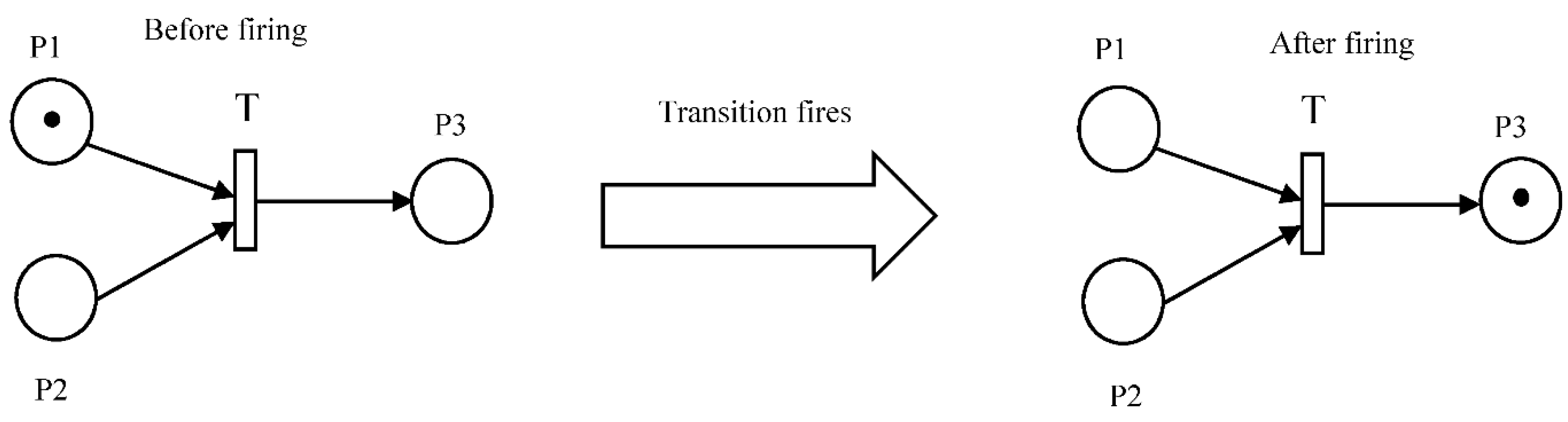
A PN is a graphical tool used to model and interpret complex systems which are described as concurrent, distributed, stochastic and/or non-deterministic. The tool itself was first developed by Carl Petri as part of his PhD dissertation [35] to discover suitable solutions for a precise theory of communication. A PN is similar to a flowchart or block diagram in function. It consists of four fundamental graphical features, namely: places, transitions, arcs and tokens [36]. Places are denoted by a circle representing the state of a component or system. Transitions, denoted by a rectangle, are what make modelling of a system’s dynamic behavior possible and, therefore, allow the system to change its state. Tokens are small solid circles which are situated inside places and have markings to represent the state of the system. Arcs are solid arrows which connect places to transitions. An arc which is drawn from a place to a transition is called an input arc, whereas an arc drawn in the opposite direction is known as an output arc [37]. The system will change its state when a token is transferred from an input place to an output place. This is made possible through the “firing” of an “enabled” transition [38]. A transition is enabled (or activated) when certain requirements are met. An example of this would be a transition only being enabled when there is a token in one of its input places. If there happens to be a delay associated with that transition, then it will only fire after that delay has elapsed even if it is enabled. This is shown in Figure 3. The transition T is enabled because there is a token present in the place P1 and fires only after a delay of time t has elapsed. The transition referred to in this example is known as a timed transition. A transition without any delay is referred to as an immediate transition.
The main properties of a PN model are:
Accessibility: this refers to the state which can be attained during the operation of a system.
Activity: this represents the ability of a system to operate as normal.
Boundary: this refers to the conditions under which a system can operate normally.
Conservation: this represents the resource restriction in a system.
Consistency: this refers to the lack of conflict which exists between the system’s behavior.
Fairness: this indicates that a system is starvation-free, i.e., that necessary resources are available.
Resilience: this refers to the capacity of a system to be periodic, i.e., to recur at intervals.
Reversibility: this refers to the ability of a system to return to its initial state.
The standard PN model does not perform reliability analysis of a system with respect to changes in time. This means that transitions here fire immediately, i.e., without any delay. Therefore, the PN model will include a finite sequence of five elements [39]. These elements are represented as follows:
where is a finite set of places, is a finite set of transitions, is a set of arcs, is a weight function, and is the initial marking with .
Although the standard PN model is a useful graphical and mathematical tool for modelling and analyzing the behavior of systems, it does not take ‘time’ into account. To this end, a subclass of PN models called stochastic Petri net (SPN) was proposed [38]. The SPN, on which our model relies, is a type of PNs which takes the concept of time into account. This is important because it helps to model and analyze the dynamic behavior of systems. The transitions for SPNs have firing times which can be deterministic, normally distributed or exponentially distributed random variables, meaning that the transitions fire after a time delay. A SPN is represented by a 6-tuple as follows:
where and are defined as in Equation (1), and is the set of transition firing rates.
3.2. The Stochastic Petri Net (SPN)-Based O&M Planning Model
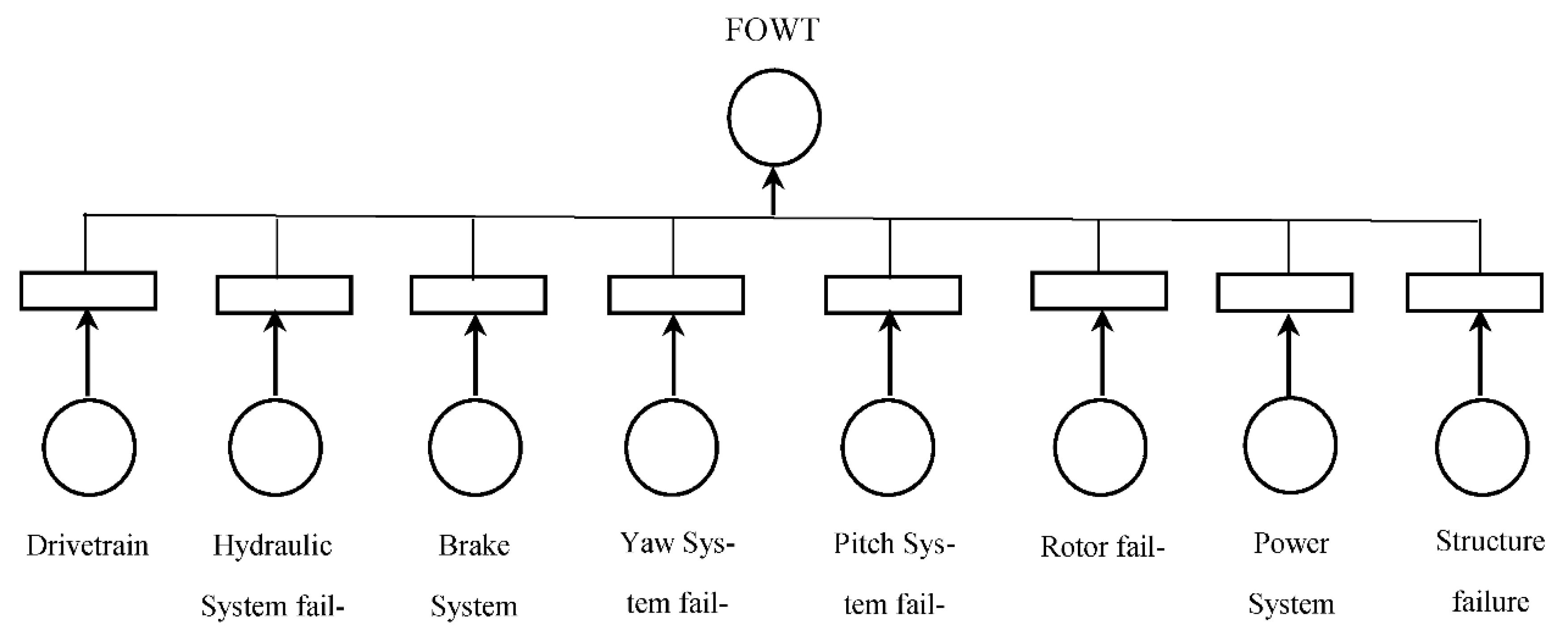
Due to the complex nature of the FOWTs and their support structures, we divided the system into eight subsystems including drivetrain unit, hydraulic system, brake system, yaw system, pitch system, rotor system, power system and structural components. These subsystems include a number of components, as listed in Table 2.
The eight subsystems are considered to be connected in series with each other, meaning that the wind turbine cannot function if any of these components fails. The PN model of the overall system is represented in Figure 4. The primary aim of our model is to present the degradation process of each component. The maintenance strategy applied to FOWT system is CBM, and the maintenance is conducted when the condition of a sub-assembly reaches its degraded state. For the purpose of simplicity, the following assumptions are made:
- The CMS equipment is in a good working condition;
- The maintenance restores the condition of each sub-assembly to “normal” or “as good as new” state;
- Wind speed is within the necessary operating range of the wind turbine.
The software tool used to develop the SPN model for O&M planning of FOWTs is TimeNET Version 4 [40]. TimeNET was designed by the Real-Time Systems and Robotics group at the Technische Universität Berlin, Germany, as an interface to model the SPNs with non-exponentially distributed firing times.
3.2.1. Modelling the Degradation Process
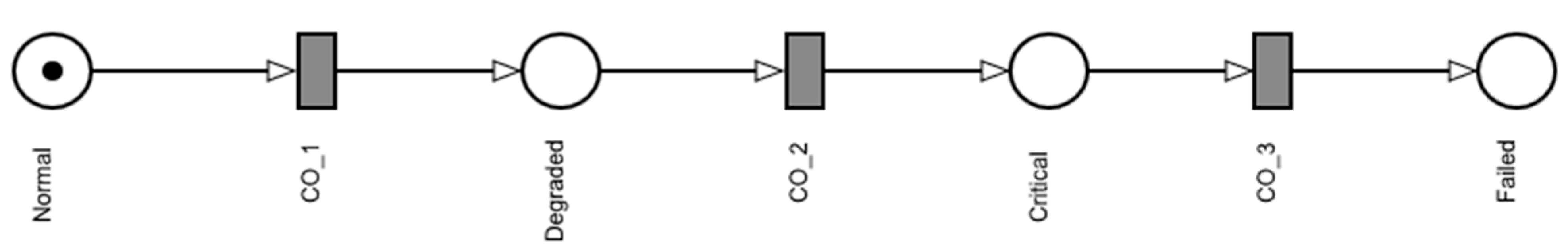
To model the degradation process of components, four states are defined: (i) normal state, (ii) degraded state, (iii) critical state, and (iv) functional failure state. The transitions linking these states represent events which take place for one state to progress into another, i.e., for the components to degrade from the normal to degraded to critical and finally to the functional failure state. The times associated with each transition represents how long it takes for the condition of the components to further progress. The model begins with the token residing in the Normal place. This signifies that the sub-assembly is operating as it normally should be. The presence of this token enables the transition CO_1 (Continued Operation 1) to fire, transferring the token to the Degraded place after a delay represented by a Weibull distribution with shape parameter β and scale parameter η (in this study, the scale parameter is represented in years). The movement of the token in this instance signifies the change in the asset’s condition; therefore, the token being situated within the Degraded place signifies that the asset is in a degraded state.
As we assume that the resources (including transport vessels, service crew, spare parts and special tools) are available, the maintenance tasks begin immediately after the condition of a component is identified as ‘degraded’. In an event that resources might not be available for a maintenance task, the transition CO_2 becomes enabled and fires, transferring the token from the Degraded place to the Critical place. The critical state in this model serves to notify the operators that functional failure will occur if no maintenance is performed. This process then continues until the token ends up in the Failed place. By default, this then prompts replacement of the component. The degradation process on TimeNET is shown in Figure 5.
3.2.2. Modelling the Condition Monitoring Process
The CMS is utilized to continuously monitor and report the condition of FOWT components during operation. This process identifies and reveals any changes to the asset’s condition based on pre-specified operational and performance metrics. Therefore, the CMS plays an extremely important role as the maintenance actions are taken based on alarm conditions. With the components working in normal condition (i.e., the token placed in the Normal place), any changes to the condition can be identified by the CMS. This will enable the aforementioned immediate transitions, depositing the tokens into either the normal, degraded, critical or failed places. This then reveals the known condition of the component at that point in time. Thus, this is the condition of a component that determines whether a maintenance action is required to be performed or not. The accuracy of the CMS is also important, as monitoring equipment like many other machines are prone to errors or faults. When there is an error in the CMS, the condition of components will be reported wrongly to operators, which may lead to either initiating a maintenance action when it is not needed or holding back a maintenance action when it is needed.
3.2.3. Modelling the Maintenance Process
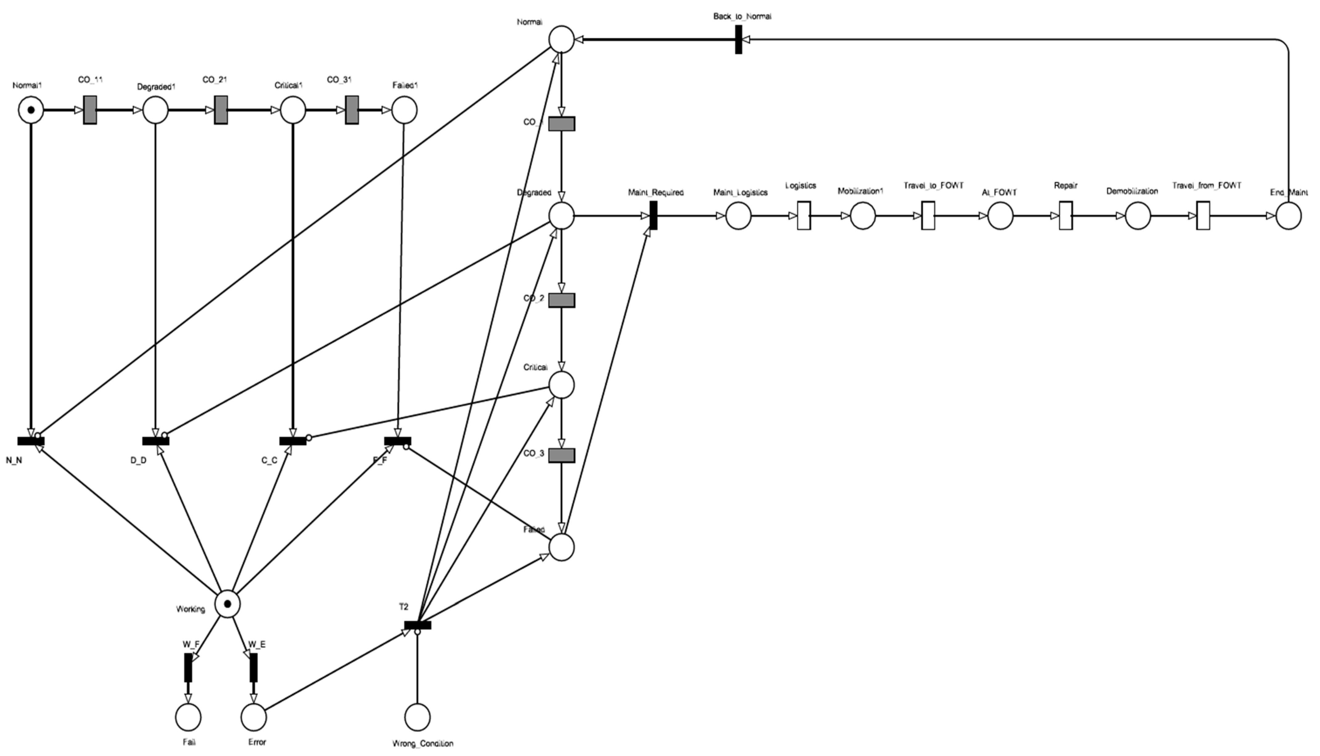
The maintenance process includes several key stages including: maintenance logistics, maintenance resource mobilization, actual repair/replacement, resource demobilization and end of maintenance activities. These stages are represented by the Maint_Logistics, Mobilization, At_FOWT, Demobilization and End_Maint states, which are all shown in Figure 6. The transitions linking these states represent the events which have to occur for the maintenance process to progress from one state to the next. The model has been set up such that each transition in this maintenance process can only become enabled if a token is present in the place which precedes it. When it becomes enabled, the transition can only fire after a delay of time t. This delay is governed by the type of maintenance being performed on any particular component. Types of maintenance actions for wind turbines are explained in Table 3.
When the condition of a component reaches the Degraded state, the maintenance process begins and the immediate transition Start_Maint_Process is fired. This transfers the token from the Degraded place and deposits it in the Maint_Logistics place. The transition Logistics is then enabled and fires only after a delay representing the logistics time has elapsed. The token is then deposited in the Mobilization place. As a result of this, the transition Travel_to_FOWT is enabled and fires only after a delay representing the travel time to the floating offshore wind farm. This then places the token in the At_FOWT place. This process continues until the maintenance process is completed with the token situated at the End_Maint place, enabling the transition Back_to_Normal which fires immediately. The token is finally deposited in the Normal place, signifying that the component has resumed normal operations. The PN model, including the degradation process, maintenance process and condition monitoring process, for the FOWT system is shown in Figure 6.
4. Results and Discussion
In this section, the proposed SPN model is applied to O&M planning of an NREL 5 MW spar buoy floating wind turbine system with an anticipated design lifetime of 25 years. The data for simulation of degradation and maintenance processes of FOWT components were collected from the literature as well as wind energy industry databases. These data are given in the Appendix A, Appendix B and Appendix C. Appendix A presents the types of maintenance actions adopted for the FOWT components. Appendix B presents the Weibull distribution parameters for each stage of FOWT degradation. As can be seen in Appendix B, the shape parameters (β) for FOWT components are greater than 1, meaning that the failure rates of components consistently increase with time. Appendix C shows the parameters adopted for the maintenance of the FOWT based on each maintenance type.
In the context of this research, maintenance/repair is assumed to begin when the component reaches the Degraded state. After performing the maintenance, the component is assumed to get back to the normal state or as-good-as-new, meaning that the time interval begins when the component starts operating and ends when the repair starts. The activities performed during the repair/replacement process depends on the maintenance strategy adopted for that component. The simulation results are analyzed to obtain other pertinent metrics such as the time to failure, expected number of repairs/interventions, and the repair/maintenance costs. These performance metrics for each component are then combined to determine the performance of the entire system.
4.1. Component Maintenance Prediction
Given that maintenance is performed when CMS identifies the component condition as ‘degraded’, the time at which a repair must be initiated can be determined. By estimating the number of times each component reaches a degraded state over its lifetime, the total number of maintenance interventions can be calculated.
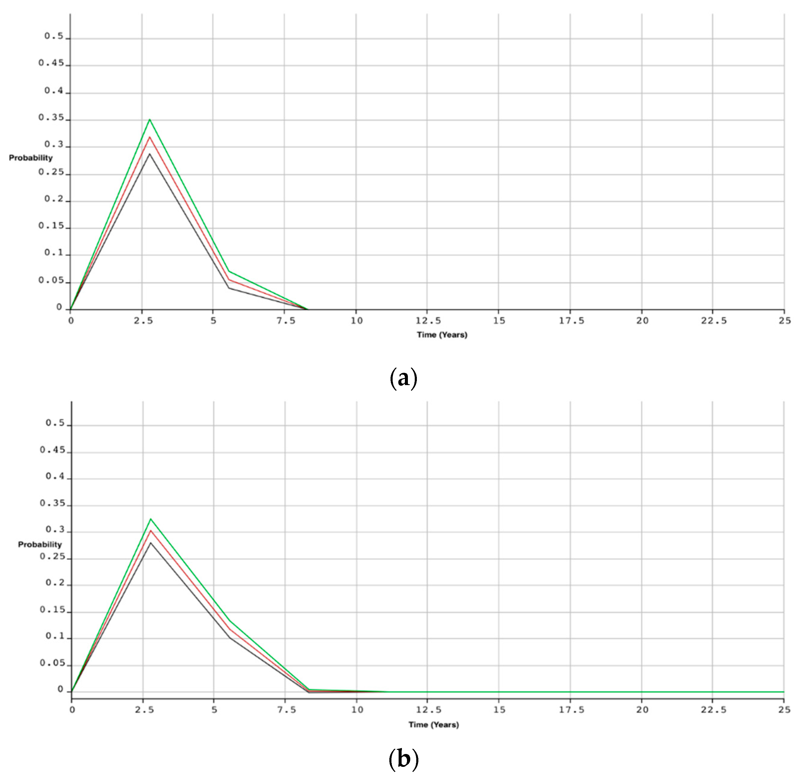
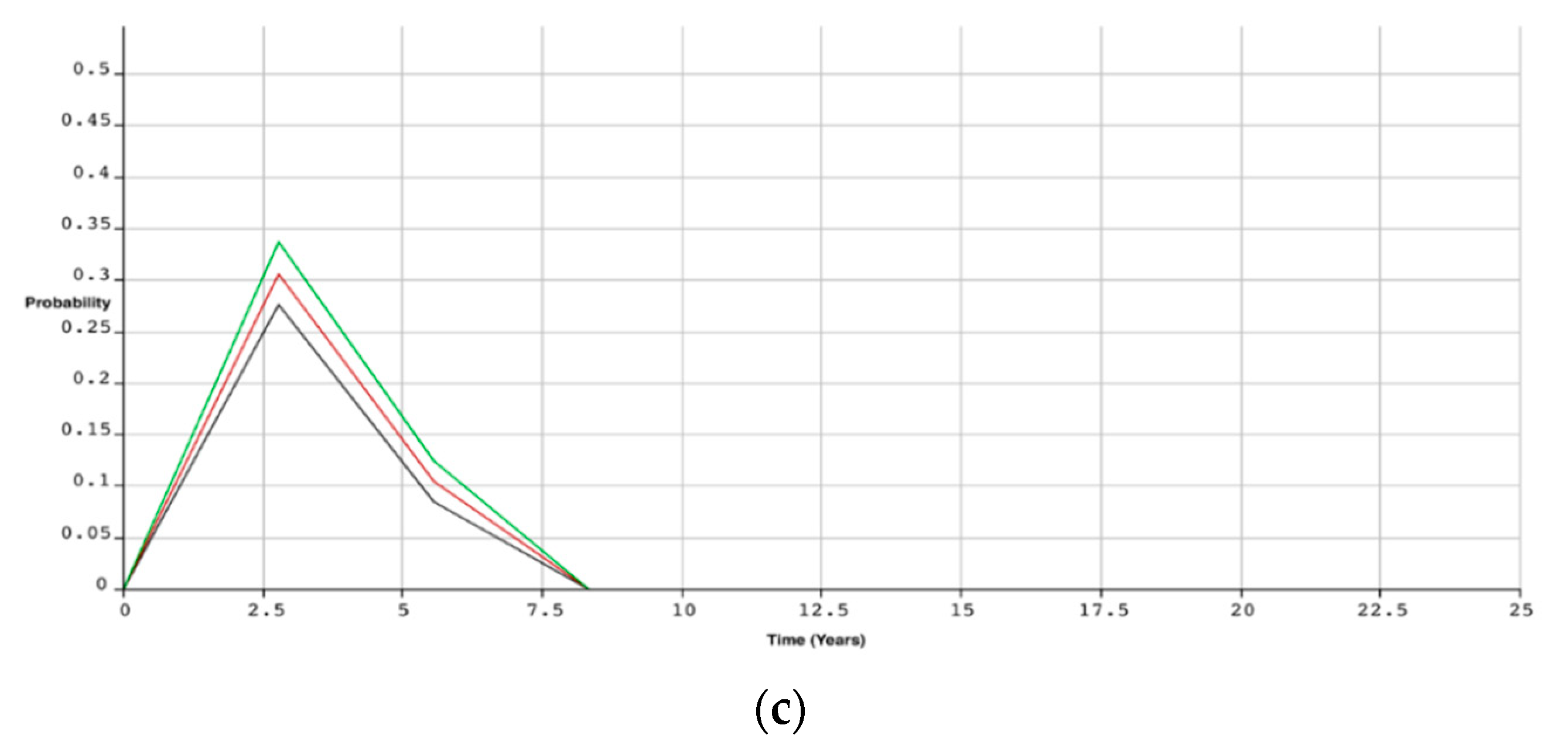
Taking the FOWT mooring system as an example, Figure 7 presents the probability of the component being in a particular state over time. In the three plots shown, we have reported the probability of each of the three mooring lines being in the degraded state over time. In each plot, three lines are presented as there is a 95% confidence interval integrated into the analysis. The topmost (green) line represents the upper limit, the middle (red) line represents the mean, and the bottom (black) line represents the lower limit. The simulation results show that the three mooring lines reach a degraded state after 8.33 years, 11.11 years and 8.33 years, respectively. The dominant failure mode of the mooring system is wearing, which becomes critical when it reaches a limit. This then triggers a maintenance which in this case is the type 4 maintenance, restoring the system to as-good-as-new or normal condition. It therefore follows that the three mooring lines will be repaired 3 times, 2.25 times and 3 times over 25-year lifetime, respectively. Table 4 shows the average length of time that it takes for each component of the FOWT system to reach a degraded state. This can then be used to predict the total number of maintenances which will need to be performed over the wind farm lifetime.
4.2. Maintenance Cost Prediction
The cost of maintenance for each FOWT component depends on the type of maintenance adopted for that component. In this paper, four maintenance types were considered as listed in Table 3. The costs associated with each type of maintenance include: labor cost, material cost and logistics cost. The total maintenance cost for each FOWT component is obtained by multiplying the cost of each maintenance by the expected number of maintenance performed on that component over the wind farm lifetime. The expected number of repairs and associated costs (in monetary unit) for all FOWT components are given in Table 4.
The analysis shows that the power converter is the most contributing component to the O&M cost of FOWTs, followed by structural components including anchors, mooring lines, tower and nacelle.
4.3. System Downtime
The FOWT system experiences downtime when a maintenance is performed. The downtime in this case is defined as the time between when the degradation is detected and the repair task is completed. This encompasses the logistics time to prepare personnel, parts and equipment, time to travel to and from the FOWT and the actual repair time. It should be noted that the system downtime does not consider the weather waiting time and the duration between the time when a degradation occurs and it is detected. Weather waiting time is a function of the environmental conditions wherein the wind farm is situated. The downtime for each component is a function of the maintenance type.
Our results show that the highest system downtime (26.63 days) is attributed to the maintenance of the power converter, whereas the lowest system downtime (1.75 days) is attributed to the maintenance of the rotor blades, tower and nacelle. The average downtime caused by all components is estimated to be 5.65 days. This information can be used to determine the annual loss in energy production as a result of component degradation or failure.
4.4. Sensitivity Analysis
A sensitivity analysis is performed to understand the impact of CMS on system performance. In the proposed model, the CMS was assumed to be in perfect working condition. However, the CMS itself may experience downtime due to technical problems. In this study, the annual failure rate of the CMS is assumed to be 0.006. Table 5 shows the effect of the CMS failure rate on the mooring lines, power generator and yaw bearings. As can be seen, the probability of each component failing increases when the CMS failure rate is incorporated into the model. This implies that the condition of the CMS should also be a point of focus when planning O&M activities in floating offshore wind farms as it can affect the asset’s operation.
5. Conclusions
This paper presented a stochastic Petri network (SPN) model for O&M planning of floating offshore wind turbines (FOWTs) and their support structures. The model encompassed the degradation processes, maintenance operations and condition monitoring system (CMS) for eight subassemblies of the floating offshore wind turbines. The expected number of failures in each component over its lifetime was predicted based on how often the component reaches its degraded state. The number and cost of maintenance interventions for each component as well as the entire system were predicted over the wind farm’s lifetime with the yaw actuator and brake discs having the most expected number of repairs. However, the power converter was identified as the most expensive component to maintain when factoring the number of maintenance interventions and cost of each intervention.
The system downtime was also analyzed, with different factors involved. The highest contributor to system downtime was determined to be the power converter, while the lowest contributors to downtime were the rotor blades, tower, nacelle and mooring lines. It was determined that maintenance effort should be focused on power converters as they were the most expensive component to maintain and caused the longest system downtime. Finally, a sensitivity analysis was performed to analyze the effect of the CMS on each component’s performance. The analysis shows that the probability of failure of the component is lower with the CMS having higher reliability.
Further studies can be undertaken on maintenance and degradation modelling of FOWTs using other advanced techniques such as Dynamic Bayesian Networks and the Markov process. The submarine power cables were excluded from this study due to unavailability of failure and maintenance data. The model developed in this paper can be extended to include power cables when data become available in future. Mooring lines can also be focused on in more detail with regards to O&M planning as its use in the wind energy industry is still relatively in its infancy. Lastly, the proposed model can also be applied towards O&M planning of other complex assets in both the onshore and offshore sectors.
Author Contributions
Conceptualization, T.E., M.S., T.A. and F.D.; methodology, T.E.; software, T.E.; validation, T.E., M.S. and F.D.; formal analysis, T.E.; investigation, T.E. and T.A.; resources, M.S.; data curation, T.E.; writing—original draft preparation, T.E., M.S., F.D.; writing—review and editing, T.E., M.S., T.A. and F.D.; visualization, T.E. and T.A.; supervision, M.S.; project administration, T.A.; funding acquisition, M.S. All authors have read and agreed to the published version of the manuscript.
Funding
This research was funded by the EPSRC Supergen Wind Hub in a project titled “Stochastic Methods and Tools to Support ‘Real-Time’ Planning of Risk-based Inspection for Offshore Wind Structures”.
Institutional Review Board Statement
Not applicable.
Informed Consent Statement
Not applicable.
Data Availability Statement
Not applicable.
Conflicts of Interest
The authors declare no conflict of interest.
Appendix A

Table A1.
Type of maintenance actions adopted in floating offshore wind turbines [36].
Table A1.
Type of maintenance actions adopted in floating offshore wind turbines [36].
| Subsystem | Component | Type of Maintenance | Description of Maintenance Action |
|---|---|---|---|
| Drivetrain | Bearing | 3 | Pitting replacement |
| Gearbox | 3 | Gear tooth repair | |
| Shaft | 3 | Minor repair | |
| Hydraulic | Pump | 2 | Part replacement |
| Valves/Pipes | 3 | Replacement | |
| Braking | Callipers/Pads | 2 | Replace worn component |
| Discs | 2 | Replacement | |
| Yaw | Actuator | 3 | Minor repair |
| Bearing | 3 | Corrective repair | |
| Brake | 2 | Replacement | |
| Pitch | Actuator | 3 | Part replacement |
| Bearing | 3 | Minor repair | |
| Rotor | Hub | 3 | Minor corrosion repair |
| Blade | 4 | Minor repair | |
| Power | Generator | 2 | Part replacement |
| Frequency Converter | 1 | Part/complete replacement | |
| Transformer | 2 | Part/complete replacement | |
| Structure | Tower | 4 | Corrosion repair |
| Nacelle | 4 | Crack repair | |
| Mooring Lines | 4 | Wear repair |
Appendix B
| Subsystem | Component | Failure Rate (λ) | Degraded Condition | Critical Condition | Functional Failure | |||
|---|---|---|---|---|---|---|---|---|
| Shape | Scale (year) | Shape | Scale (year) | Shape | Scale (year) | |||
| Drivetrain | Bearing | 0.0050 | β = 1.2 | η = 160 | β = 1.5 | η = 20 | β = 1.5 | η = 20 |
| Gearbox | 0.0500 | β = 1.3 | η = 16 | β = 1.2 | η = 2 | β = 1.4 | η = 2 | |
| Shaft | 0.0050 | β = 1.2 | η = 160 | β = 1.5 | η = 20 | β = 1.5 | η = 20 | |
| Hydraulic | Pump | 0.0500 | – | – | β = 1.2 | η = 20 | ||
| Valves/Pipes | 0.0610 | β = 1.2 | η = 13.11 | – | β = 1.2 | η = 3.28 | ||
| Braking | Callipers/Pads | 0.0610 | β = 1.2 | η = 13.11 | – | β = 1.2 | η = 3.28 | |
| Discs | 0.0189 | β = 1.2 | η = 42.28 | – | β = 1.2 | η = 10.57 | ||
| Yaw | Actuator | 0.0189 | β = 1.2, | η = 42.28 | – | β = 1.2 | η = 10.57 | |
| Bearing | 0.0275 | β = 1.2 | η = 29.12 | β = 1.2 | η = 3.64 | β = 1.2 | η = 3.64 | |
| Brake | 0.0275 | β = 1.2 | η = 29.12 | β = 1.2 | η = 3.64 | β = 1.2, | η = 3.64 | |
| Pitch | Actuator | 0.0275 | β = 1.2, | η = 29.12 | – | β = 1.2 | η = 7.28 | |
| Bearing | 0.0520 | β = 1.2, | η = 15.38 | β = 1.2 | η = 1.92 | β = 1.2 | η = 1.92 | |
| Rotor | Hub | 0.0520 | β = 1.2 | η = 15.38 | β = 1.2 | η = 1.92 | β = 1.2 | η = 1.92 |
| Blade | 0.0348 | β = 1.2 | η = 23.02 | β = 1.2 | η = 2.88 | β = 1.2 | η = 2.88 | |
| Power | Generator | 0.0520 | β = 1.2 | η = 15.38 | β = 1.2 | η = 1.92 | β = 1.2 | η = 1.92 |
| Frequency Converter | 0.0240 | β = 1.2 | η = 33.38 | – | β = 1.2 | η = 8.35 | ||
| Transformer | 0.0670 | – | – | β = 1.2 | η = 14.93 | |||
| Structure | Tower | 0.0670 | – | – | β = 1.2 | η = 14.93 | ||
| Nacelle | 0.0060 | β = 1.2 | η = 133.33 | β = 1.2 | η = 16.67 | β = 1.2 | η = 16.67 | |
| Mooring Line 1 | 0.0136 | β = 1.2 | η = 58.0 | β = 1.2 | η = 7.25 | β = 1.2 | η = 7.25 | |
| Mooring Line 2 | 0.0381 | β = 1.2 | η = 21.0 | β = 1.2 | η = 2.63 | β = 1.2 | η = 2.63 | |
| Mooring Line 3 | 0.0262 | β = 1.2 | η = 31.0 | β = 1.2 | η = 3.89 | β = 1.2 | η = 3.89 | |
| Anchor | 0.0344 | β = 1.2 | η = 23.02 | β = 1.2 | η = 2.88 | β = 1.2 | η = 2.88 | |
Appendix C
Table A3.
Maintenance parameters for floating offshore wind turbines [37].
Table A3.
Maintenance parameters for floating offshore wind turbines [37].
| Maintenance Type | Logistic Time (h) | Repair Time (h) | Travel Time to Wind Turbine (h) | Travel Time from Wind Turbine (h) |
|---|---|---|---|---|
| 1 | 160 | 50 | 1.5 | 1.5 |
| 2 | 48 | 10 | 1.5 | 1.5 |
| 3 | 24 | 3 | 1.5 | 1.5 |
| 4 | 8 | 3 | 1.5 | 1.5 |
References
- Wind Europe. Wind Energy in Europe in 2019: Trends and Statistics. 2020. Available online: https://windeurope.org/ (accessed on 18 September 2020).
- European Commission. Transforming the European Energy System through INNOVATION: Integrated SET Plan Progress in 2016; Publications Office of the European Union: Luxembourg, 2016. [Google Scholar]
- Hernández, C.V.; Telsnig, T.; Pradas, A.V. JRC Wind Energy Status Report. 2017. Available online: https://setis.ec.europa.eu/sites/default/files/reports/wind_energy_status_report_2016.pdf (accessed on 3 March 2019).
- GOV.UK. New Plans to Make UK World Leader in Green Energy. 2020. Available online: https://www.gov.uk/government/news/new-plans-to-make-uk-world-leader-in-green-energy (accessed on 6 October 2020).
- The Crown Estate. Offshore Wind Operational Report. 2019. Available online: https://www.thecrownestate.co.uk/media/3515/offshore-wind-operational-report-2019.pdf (accessed on 18 September 2020).
- WindEurope. Offshore Wind in Europe: Key Trends and Statistics 2019. 2020. Available online: https://windeurope.org/wp-content/uploads/files/about-wind/statistics/WindEurope-Annual-Offshore-Statistics-2019.pdf (accessed on 18 September 2020).
- Shafiee, M.; Brennan, F.; Espinosa, I.A. A parametric whole life cost model for offshore wind farms. Int. J. Life Cycle Assess. 2016, 21, 961–975. [Google Scholar] [CrossRef] [Green Version]
- Shafiee, M. Maintenance logistics organization for offshore wind energy: Current progress and future perspectives. Renew. Energy 2015, 77, 182–193. [Google Scholar] [CrossRef]
- Shafiee, M.; Stamelos, G.; Aziminia, M.M.; Elusakin, T.; Adedipe, T.; Dinmohammadi, F. Failure Analysis of Floating Offshore Wind Turbine Technologies. In Proceedings of the 4th International Conference on Renewable Energies Offshore (RENEW), Lisbon, Portugal, 12–15 October 2020. [Google Scholar]
- Carbon Trust. Floating Offshore Wind: Market and Technology Review. 2015. Available online: https://prod-drupal-files.storage.googleapis.com/documents/resource/public/Floating%20Offshore%20Wind%20Market%20Technology%20Review%20-%20REPORT.pdf (accessed on 18 September 2020).
- Roddier, D.; Cermelli, C.; Weinstein, A. Windfloat: A Floating Foundation for Offshore Wind Turbines—Part I: Design Basis and Qualification Process. In Proceedings of the ASME 2009 28th International Conference on Ocean, Offshore and Arctic Engineering, Honolulu, HI, USA, 31 May–5 June 2009; pp. 845–853. [Google Scholar] [CrossRef]
- Jonkman, J.M.; Matha, D. Dynamics of offshore floating wind turbines-analysis of three concepts. Wind Energy 2011, 14, 557–569. [Google Scholar] [CrossRef]
- Equinor. Hywind—The World’s Leading Floating Offshore Wind Solution. 2018. Available online: https://www.equinor.com/en/what-we-do/hywind-where-the-wind-takes-us.html (accessed on 18 September 2020).
- Principle Power. WindFloat. 2015. Available online: https://www.offshorewind.biz/2018/07/11/hengtong-lands-windfloat-atlantic-export-cable-deal/ (accessed on 3 March 2019).
- Sway Concept. Available online: http://www.sway.no/?page=166 (accessed on 3 March 2019).
- Scottish Renewables. Floating Wind: The UK Industry Ambition. 2019. Available online: https://www.scottishrenewables.com/assets/000/000/475/floating_wind_the_uk_industry_ambition_-_october_2019_original.pdf?1579693018 (accessed on 1 December 2019).
- Durakovic, A. Europe’s Most Powerful Wind Turbine Sits Atop Floating Foundation. 2020. Available online: https://www.offshorewind.biz/2020/11/11/europes-most-powerful-wind-turbine-sits-atop-floating-foundation/ (accessed on 11 November 2020).
- Shafiee, M.; Finkelstein, M. An optimal age-based group maintenance policy for multi-unit degrading systems. Reliab. Eng. Syst. Saf. 2015, 134, 230–238. [Google Scholar] [CrossRef]
- Shafiee, M.; Finkelstein, M. A proactive group maintenance policy for continuously monitored deteriorating systems: Application to offshore wind turbines. Proc. Inst. Mech. Eng. Part O J. Risk Reliab. 2015, 229, 373–384. [Google Scholar] [CrossRef]
- Adedipe, T.; Shafiee, M. An economic assessment framework for decommissioning of offshore wind farms using a cost breakdown structure. Int. J. Life Cycle Assess. 2021. [Google Scholar] [CrossRef]
- Jeon, S.H.; Cho, Y.U.; Seo, M.W.; Cho, J.R.; Jeong, W.B. Dynamic response of floating substructure of spar-type offshore wind turbine with catenary mooring cables. Ocean Eng. 2013, 72, 356–364. [Google Scholar] [CrossRef]
- Leigh, J.M.; Dunnett, S.J. Use of Petri nets to model the maintenance of wind turbines. Qual. Reliab. Eng. Int. 2016, 32, 167–180. [Google Scholar] [CrossRef] [Green Version]
- Shafiee, M.; Sørensen, J.D. Maintenance optimization and inspection planning of wind energy assets: Models, methods and strategies. Reliab. Eng. Syst. Saf. 2019, 192, 105993. [Google Scholar] [CrossRef]
- Adedipe, T.; Shafiee, M.; Zio, E. Bayesian network modelling for the wind energy industry: An overview. Reliab. Eng. Syst. Saf. 2020, 202, 107053. [Google Scholar] [CrossRef]
- Garbatov, Y.; Soares, C.G. Bayesian updating in the reliability assessment of maintained floating structures. J. Offshore Mech. Arct. Eng. 2002, 124, 139–145. [Google Scholar] [CrossRef]
- Cross, P.; Ma, X. Model-based and fuzzy logic approaches to condition monitoring of operational wind turbines. Int. J. Autom. Comput. 2015, 12, 25–34. [Google Scholar] [CrossRef] [Green Version]
- Koh, J.H.; Ng, E.Y.K. Downwind offshore wind turbines: Opportunities, trends and technical challenges. Renew. Sustain. Energy Rev. 2016, 54, 797–808. [Google Scholar] [CrossRef]
- Choy, C.C.; Schafhirt, S.; Muskulus, M. Markov Approach to Estimate Fatigue Damage for Monopile-Based Offshore Wind Turbines. In Proceedings of the 28th International Ocean and Polar Engineering Conference, Sapporo, Japan, 10–15 June 2018; pp. 287–293. [Google Scholar]
- Li, J.; Zhang, X.; Zhou, X.; Lu, L. Reliability assessment of wind turbine bearing based on the degradation-Hidden-Markov model. Renew. Energy 2019, 132, 1076–1087. [Google Scholar] [CrossRef]
- Marseguerra, M.; Zio, E.; Podofillini, L. Condition-based maintenance optimization by means of genetic algorithms and Monte Carlo simulation. Reliab. Eng. Syst. Saf. 2002, 77, 151–165. [Google Scholar] [CrossRef]
- Van Bussel, G.J.; Bierbooms, W.A.A.M. The DOWEC offshore reference windfarm: Analysis of transportation for operation and maintenance. Wind Eng. 2003, 27, 381–392. [Google Scholar] [CrossRef]
- Kusiak, A.; Verma, A. Analyzing bearing faults in wind turbines: A data-mining approach. Renew. Energy 2012, 48, 110–116. [Google Scholar] [CrossRef]
- Zurawski, R.; Zhou, M. Petri nets and industrial applications—A tutorial. IEEE Trans. Ind. Electron. 1994, 41, 567–583. [Google Scholar] [CrossRef]
- Yang, X.; Li, J.; Liu, W.; Guo, P. Petri net model and reliability evaluation for wind turbine hydraulic variable pitch systems. Energies 2011, 4, 978–997. [Google Scholar] [CrossRef] [Green Version]
- Petri, C.A. Kommunikation mit Automaten. Ph.D. Thesis, University of Hamburg, Hamburg, Germany, 1962. [Google Scholar]
- Murata, T. Petri nets: Properties, analysis and applications. Proc. IEEE 1989, 77, 541–580. [Google Scholar] [CrossRef]
- Le, B.; Andrews, J. Modelling wind turbine degradation and maintenance. Wind Energy 2016, 19, 571–591. [Google Scholar] [CrossRef]
- Elusakin, T.; Shafiee, M. Reliability analysis of subsea blowout preventers with condition-based maintenance using stochastic Petri nets. J. Loss Prev. Process Ind. 2020, 63, 104026. [Google Scholar] [CrossRef]
- Liu, Z.; Yonghong, Y.; Cai, B.; Liu, X.; Li, J.; Tian, X.; Ji, R. RAMS analysis of hybrid redundancy system of subsea blowout preventer based on stochastic petri nets. Int. J. Secur. Appl. 2013, 7, 159–166. [Google Scholar]
- Zimmermann, A.; Knoke, M. TimeNET 4.0 User Manual, Technical Report, Technische Universität Berlin. 2007. Available online: http://www.eecs.tu-berlin.de/fileadmin/f4/TechReports/2007/2007-13.pdf (accessed on 3 March 2019).
- Ciang, C.C.; Lee, J.-R.; Bang, H.-J. Structural health monitoring for a wind turbine system: A review of damage detection methods. Meas. Sci. Technol. 2008, 19, 122001-1–122001-20. [Google Scholar] [CrossRef] [Green Version]
- Hahn, B.; Durstewitz, M.; Rohrig, K. Reliability of Wind Turbines. In Wind Energy; Springer: Berlin, Germany, 2007; pp. 329–332. [Google Scholar]

Figure 2.
Spar-type floating offshore wind turbine [21].
Figure 2.
Spar-type floating offshore wind turbine [21].

Figure 3.
Representation of a Petri network model.

Figure 4.
Petri network model for FOWT system failure.

Figure 5.
Degradation model on TimeNET.

Figure 6.
TimeNET model of component degradation and maintenance process for FOWTs.

Figure 7.
The performance of three mooring lines in a degraded state (a) line 1, (b) line 2, (c) line 3.
Figure 7.
The performance of three mooring lines in a degraded state (a) line 1, (b) line 2, (c) line 3.


Table 1.
Comparison of Petri network (PN) model with other analytics tools.
| Characteristics | Other Techniques | PN |
|---|---|---|
| Quality of output values | Fuzzy models require defuzzification to generate outputs. | The PN model does not require any extra analysis to generate outputs. |
| Long-term operation and maintenance (O&M) modelling | Markov models do not truly represent long-term wind turbine performance as they use parodic inspection data and sometimes include simplistic assumptions. | The PN model can easily represent long-term wind turbine degradation as well as maintenance processes. |
| Modelling with limited/unavailable data | Simulation models are significantly dependent on the availability of input data such as failure and repair information which might be unavailable for some floating offshore wind turbines. | The PN model is able to predict the degradation of systems by utilizing Weibull distributions for time-to-failure characterisations, overcoming the concerns of limited/unavailable data. |
| Complexity of technique | The BN model can become quite complex as conditional probability table (CPT) entries must be set for each variable. | In the PN model, the parameters which need to be set are the firing rates of timed transitions, which are equivalent to Weibull distribution parameters. |
| Class imbalance problem | Data mining models applied to wind turbines commonly succumb to the class imbalance problem which is experienced as a result of one class of data (e.g., data in failure instances) being considerably less in quantity than another class of data (e.g., data in normal instances). This problem hinders the predictive capacity of data mining models. | As the PN model does not require any meaningful amounts of wind turbine condition monitoring data for analysis, it is immune to the class imbalance problem. |
Table 2.
Floating offshore wind turbine (FOWT) subsystems and components.
| FOWT Subsystem | Component |
|---|---|
| Drivetrain unit | Main bearings |
| Gearbox | |
| Main shaft | |
| Hydraulic system | Gear pump |
| Valves/pipes | |
| Brake system | Callipers/pads |
| Brake discs | |
| Yaw system | Hydraulic actuator |
| Bearing/gear | |
| Yaw brake | |
| Pitch system | Hydraulic actuator |
| Bearing/gear | |
| Rotor system | Hub |
| Blades | |
| Power system | Generator |
| Frequency converter | |
| Transformer | |
| Structure | Tower |
| Floating foundation | |
| Mooring lines |
Table 3.
Types of maintenance for wind turbines [37].
Table 3.
Types of maintenance for wind turbines [37].
| Maintenance Type | Description |
|---|---|
| Type 1 | Heavy component, requires internal/external crane (>800–1000 kg) |
| Type 2 | Small parts, requires internal (<800–1000 kg) |
| Type 3 | Small parts, inside nacelle |
| Type 4 | Small parts, outside nacelle |
Table 4.
Expected number of repairs and associated costs.
| Subsystem | Component | Type of Maintenance | Cost of Repair Type (MU) | Time to Degraded State (Years) | Expected Number of Repair | Cost of Repair (MU) |
|---|---|---|---|---|---|---|
| Drivetrain | Bearing | 3 | 10,000 | 8.33 | 3.00 | 30,000 |
| Gearbox | 3 | 10,000 | 9.02 | 2.77 | 27,700 | |
| Shaft | 3 | 10,000 | 8.33 | 3.00 | 30,000 | |
| Hydraulic | Pump | 2 | 41,000 | 12.50 | 2.00 | 82,000 |
| Valves/Pipes | 3 | 6000 | 6.25 | 4.00 | 24,000 | |
| Braking | Callipers/Pads | 2 | 19,000 | 6.25 | 4.00 | 76,000 |
| Discs | 2 | 19,000 | 5.25 | 4.76 | 90,440 | |
| Yaw | Actuator | 3 | 12,000 | 5.25 | 4.76 | 57,120 |
| Bearing | 3 | 10,000 | 8.39 | 2.98 | 29,800 | |
| Brake | 2 | 24,000 | 8.39 | 2.98 | 71,520 | |
| Pitch | Actuator | 3 | 13,000 | 6.25 | 4.00 | 52,000 |
| Bearing | 3 | 13,000 | 9.43 | 2.65 | 34,450 | |
| Rotor | Hub | 3 | 8000 | 9.43 | 2.65 | 21,200 |
| Blade | 4 | 11,000 | 8.33 | 3.00 | 33,000 | |
| Power | Generator | 2 | 65,000 | 9.43 | 2.65 | 172,250 |
| Converter | 1 | 52,000 | 6.25 | 4.00 | 208,000 | |
| Transformer | 2 | 45,000 | 12.50 | 2.00 | ||
| Structure | Tower | 4 | 27,000 | 12.50 | 2.00 | |
| Nacelle | 4 | 12,000 | 8.33 | 3.00 | 36,000 | |
| Mooring line 1 | 4 | 10,000 | 8.33 | 3.00 | 30,000 | |
| Mooring line 2 | 4 | 10,000 | 11.11 | 2.25 | 22,500 | |
| Mooring line 3 | 4 | 10,000 | 8.33 | 3.00 | 30,000 | |
| Anchor | 1 | 55,000 | 9.38 | 2.66 | 146,600 |
Table 5.
Probability of failure of gearbox, generator and yaw bearings under with CMS.
| Probability of Component Failure | ||
|---|---|---|
| Component | CMS in Perfect Condition | CMS with Failure Rate 0.006/year |
| Mooring line 1 | 0.449 | 0.695 |
| Generator | 0.438 | 0.679 |
| Yaw bearings | 0.467 | 0.685 |
Publisher’s Note: MDPI stays neutral with regard to jurisdictional claims in published maps and institutional affiliations. |
© 2021 by the authors. Licensee MDPI, Basel, Switzerland. This article is an open access article distributed under the terms and conditions of the Creative Commons Attribution (CC BY) license (http://creativecommons.org/licenses/by/4.0/).
Share and Cite
MDPI and ACS Style
Elusakin, T.; Shafiee, M.; Adedipe, T.; Dinmohammadi, F. A Stochastic Petri Net Model for O&M Planning of Floating Offshore Wind Turbines. Energies 2021, 14, 1134. https://doi.org/10.3390/en14041134
AMA Style
Elusakin T, Shafiee M, Adedipe T, Dinmohammadi F. A Stochastic Petri Net Model for O&M Planning of Floating Offshore Wind Turbines. Energies. 2021; 14(4):1134. https://doi.org/10.3390/en14041134
Chicago/Turabian StyleElusakin, Tobi, Mahmood Shafiee, Tosin Adedipe, and Fateme Dinmohammadi. 2021. "A Stochastic Petri Net Model for O&M Planning of Floating Offshore Wind Turbines" Energies 14, no. 4: 1134. https://doi.org/10.3390/en14041134
Note that from the first issue of 2016, this journal uses article numbers instead of page numbers. See further details here.