An Application of a Risk-Based Methodology to Anticipate Critical Situations Due to Extreme Weather Events in Transmission and Distribution Grids

Abstract

Nowadays, distribution network operators are urged by regulatory authorities to reduce the load disruptions due to extreme weather events, i.e., to enhance network resilience: in particular, in Italy they are required to present a yearly plan (called “resilience plans”) describing the interventions aimed to improve network resilience. To this purpose, they need new methodologies and tools to assess the network resilience and to quantify the benefits of countermeasures. This paper proposes the application of a risk-based framework and tool to assess the impacts of extreme weather events in T&D grids, which anticipate critical network situations in presence of incumbent weather threats. To do this, the forecasting of weather events is combined with the component vulnerability models in order to predict which components are more prone to fail. Based on this set of components, the set of most risky contingencies is identified and their impacts on the distribution network in terms of unsupplied load are quantified. The major advantage of the applied methodology is its generality: in fact, it is applicable to both distribution and transmission systems as well as integrated transmission and distribution (T&D) systems, considering the peculiarities of each type of grid, in terms of operation, maintenance and component vulnerabilities. In particular, the application refers to a distribution network connected to a portion of high voltage transmission system in a mountainous zone, with focus on two major threats in the area, i.e., wet snow and fall of trees induced by combined wind and snow. The methodology also quantifies the benefits brought to the system resilience by countermeasures such as reconductoring, optimal reconfiguration or new right-of-way maintenance procedures. Simulations demonstrate the ability of the methodology to support T&D operators in an operational planning context in case of different incumbent threats.

1. Introduction

The increasing frequency of extreme weather events, affecting both distribution and transmission networks, pushes distribution system operators (DSOs) and transmission system operators (TSOs) to evaluate the impact of multiple dependent outages of components, possibly leading to blackouts, and to deploy preventive or corrective countermeasures aimed at absorbing the effects of such disruptive events and quick recovery, i.e., to increase system resilience [1,2,3,4,5,6]. In this context, for instance, the current Italian regulation [4] imposes operators to publish and update a plan for resilience enhancement on a yearly basis. Even though significant steps have been made towards a systematic approach to resilience assessment and management, the methodologies so far adopted in practice still lack a sufficient generalization capability for an integrated assessment of grid resilience to a comprehensive set of threats: in particular, the same kind of threat is analyzed by different operators using different data and models, which may result in an unfair allocation of the economic incentives supporting the implementation of the mitigation measures [5,6].

Thus, the assessment of the effects of these extreme events on the grid and their mitigation call for an in-depth and harmonized analysis of the vulnerabilities of transmission and distribution (T&D) components to natural threats, as well as of the capability of suitable countermeasures to prevent the resulting -multiple dependent contingencies.

This objective is difficult also due to the fact that distinct analyses and distinct tools are generally used to address transmission and distribution systems, hence the approaches result in decoupling even though interactions can actually occur, e.g., the outage of high vltage (HV) lines can cause the loss of supply of HV/medium voltage (MV) substations with potential loss of supply to the customers at the distribution level. Reference [1] proposes a tool to evaluate the benefits of resilience brought by the deployment of grid hardening measures: they are typically focused on the transmission system and on one or more specific threats, with ad hoc models for threats and component vulnerabilities. In [7], the authors propose a methodology to study distribution network resilience to earthquakes under two particular strategies: one that hardens substation infrastructures in order to reduce their fragility levels, and the other one that uses additional network infrastructure in the form of transfer cables to shift load between substations in case of major events.

This paper presents an application of a risk-based framework and tool [8,9] in order to anticipate critical situations in the T&D system in the presence of incumbent weather threats. The current literature on the topic, as in [1,7], focuses the study on one specific grid type (transmission or distribution) and on a single threat (e.g., strong wind). The added value of the application cases herein described consists of (1) highlighting the “comprehensive” nature of the risk-based resilience assessment and enhancement problem of the relevant adopted framework, (2) contributing to the verification of the tuning of the analytical model of component vulnerabilities. With reference to point (1), the “comprehensive” nature of the framework is clearly shown as respects: (a) a wide set of natural threats can be modelled, including their combined effects on MV and HV grids in order to identify the most likely component failures, (b) the response of the integrated T&D system to contingencies is simulated, catching the potential mutual effects between MV and HV grids, (c) analytical models for different countermeasures (reconductoring, optimal reconfiguration, etc.) are adopted, which allows to quantify their benefits to system resilience thus to facilitate cost–benefit analyses. With reference to point (2), the results of the application cases are compared against the information coming from operators’ experience, in order to verify the alignment between the analytical model outputs and the feedback from the field.

In order to highlight all these aspects, the application study analyses two different threats (i.e., wet snow events with moderate wind, and tree falls due to strong wind), which are applied to a grid model representing two MV feeders connected to a portion of the Italian EHV transmission grid. The paper is organized as follows: Section 2 recalls the basics and the formulation of the proposed comprehensive methodology for resilience assessment and enhancement and describes the modeling adopted for two specific threats taken as examples for the present paper, i.e., wet snowstorms and tree fall due to strong wind, and the vulnerability models of T&D components to these threats. Section 3 presents the T&D grid study cases. Section 4 discusses the results. In Section 5, some conclusions are drawn.

2. A Reminder of RELIEF, the Methodology and the Tool for Resilience Assessment and Enhancement

This section recalls the rationale and the main aspects related to the proposed risk-based methodology for resilience assessment, as well as the architecture of the tool to anticipate critical situations and evaluate the benefits of mitigation measures. Major details can be found in [8].

2.1. The Rationale: CIGRE Definition of Resilience and the Bow Tie Model

The resilience assessment methodology is based on the following pillars:

• The CIGRE C4.47 definition of power system resilience [10];
• The bow tie model described in [8] and aimed to conceptualize the connections between threats, component vulnerabilities, and power system contingencies,;
• An extended concept of risk, clarified below.

The recent definition of power system resilience published by CIGRE WG C4.47 “Power System Resilience” [10] has proposed a distinction among the “resilience” property, the application criteria and the system capabilities, i.e., the enabling factors to have a resilient system.

The final definition of power system resilience proposed by CIGRE WG C4.47 and published in [10] is reported below:

Power System Resilience is the ability to limit the extent, severity and duration of system degradation following an extreme event.

Power system resilience is achieved through a set of key actionable measures to be taken before, during and after extreme events, such as:

• − anticipation,
• − preparation,
• − absorption,
• − adaptation,
• − rapid recovery and
• − sustainment of critical system operation

including application of lessons learnt.

This definition is innovative with respect to most of the previous definitions from the literature [11,12] because it is more accurate in defining the details of the action of the disruptive event (characterized in terms of severity, extent and duration), and because it operates a strict separation between resilience as a property and the key measures (shock absorption, fast recovery, etc.) which allow to achieve it.

In particular, the way extreme events affect the system components and the grid response to the contingencies triggered by the events themselves are clearly explained in the bow tie model presented by the authors in [8]: natural and/or human-related threats may lead to a contingency through a set of causes exploiting vulnerabilities, while the contingency might lead to different impacts depending on the circumstances. The initial impact may, in turn, affect other vulnerabilities, starting a cascading process that may eventually result in a blackout.

2.2. The Risk-Based Modeling Approach

The overall process from threats to blackout is characterized by uncertainties, from the forecasts of threats to the uncertainty in component vulnerabilities up to the possible unexpected behaviour of power system protection, control, and defense systems’ response to the contingencies. Risk can therefore represent a valuable concept to quantify the extent, severity, and duration of system degradation.

In order to quantitatively assess the relationship between root causes (threats) and power system disturbances (contingencies), an extended concept of risk is proposed: starting from the classical concept of risk [13] as a triple (contingency, probability, impact), the methodology defines the risk as a quadruple (threat, vulnerability, contingency, impact), where the probability term is replaced by the probabilistic models associated with threats and vulnerabilities. This means that, given a threat characterized in the most general terms by the r-uple of stress variables S with values s = [s₁ … s_r], the failure probability of a component in the time interval Δt = t − t₀ is expressed as a function of the average models (over Δt) for the r-dimensional density function of stress variables S, $p_{Thr}^{\left(\Delta t\right)}\left(t_0,s_1\dots s_r,x_j\right)$, and the conditional probability function of failure over Δt, $P_{V,j}{}^{\left(\mathrm{\Delta }t\right)}\left(t_0,s_1\dots s_r,x_j\right)$, respectively, as in (1).

$$P_{F,j}\left(x_j,\mathrm{\Delta }t,t_0\right)={\displaystyle \underset{S_1}{\int }\dots {\displaystyle \underset{S_r}{\overset{}{\int }}}{P}_{V,j}{}^{\left(\mathrm{\Delta }t\right)}\left(t_0,s_1\dots s_r,x_j\right)\cdot p_{Thr}^{\left(\mathrm{\Delta }t\right)}\left(t_0,s_1,\dots ,s_r,x_j\right)d{s}_1\dots d{s}_r}$$

(1)

where x_j is the location of component j subject to the r-ple of values [s₁ … s_r].

This extended risk definition allows to link probabilistic hazard assessment (PHA) studies to security assessment (SA) analyses, focusing on the root causes of disturbances and contributing to realize an integrated analysis framework and to complement conventional security analyses based on N-1 criterion. More details are reported in [14].

The threats modeled in the methodology may range from natural disasters (ice and snow storms, pollution, lightning, earthquakes, sabotage, earthquake-induced landslides, floods, fires, tree contact, component aging) to deliberate acts of sabotage [8]. The probabilistic models for threats over an operational planning time horizon (next 24–72 h) can be derived from weather forecasting systems. The last term of (1) is calculated if one knows the dependence of the stress variable pdf on location x (spatial dependence). Under this aspect, the methodology is general and can include an accurate representation of the geospatial distribution of the stress variables in case of available data from prediction systems.

Any component is described in terms of a vulnerability function with respect to each threat. The vulnerability models in (1) are analytical models which describe the interactions between grid components and the stress variables characterizing each threat. These models can also benefit from laboratory tests (e.g., characterization of mechanical fragility curves of components). The major advantages of analytical models with respect to statistical models widely used in the current literature [15] are:

• Analytical models describe the actual physical interaction between the component and the environment; thus, they can also quantify the improvement in component behaviour due to a reinforcement measure. Instead, statistical models based on past fault events cannot quantify such improvement. This is an important aspect in order to quantify the benefits of mitigation actions;
• Statistical models can be affected by errors in classifying the root cause of a fault, especially when concurrent hazards are striking the components (e.g., wind, wet snow in presence of interfering trees). In this case, classification errors may impair the validity of the model.

Statistical models may still be the best option only when the causes of a threat are not completely known or when a suitable analytical model to describe these causes is not mature.

Each threat can cause the failure of one or more components, which in turn can determine the intervention of primary and possibly backup protection systems. The failures of components followed by the intervention of primary and/or backup protection systems is called “contingency” henceforth. The set of contingencies to be analyzed in depth is found through two main steps:

• Identification of critical components using a cumulative sum screening technique (i.e., critical components are the ones whose cumulative failure probability equals a fraction δ of the cumulative failure probability of all components) [16];
• Screening of the riskiest contingencies, exploiting fast impact assessment techniques based on topological metrics [17].

An exhaustive set of single and multiple contingencies is generated by an enumeration technique, starting from critical components [8]. In particular, the methodology accounts for common mode and dependent events when analyzing multiple N-k (k > 1) contingencies. Common mode events (e.g., outage of k branches subject to the same storm) are studied considering the available geo-spatial model of the threat affecting the grid area under investigation. Dependent events are (a) busbar contingencies (also accounting for protection malfunctioning), (b) contingencies of multiple generating units within a single power plant and (c) double circuit line outages.

Contingencies are subsequently screened on the basis of ex-ante risk indicators, obtained by combining event probability with “fast” impact metrics, e.g., the number of outage-affected components or topological metrics [17].

2.3. Modeling the Response of Distribution Network and Transmission System

The response of the integrated T&D system to the retained contingencies is simulated by means of a quasi-steady state simulator of cascading outages. Even though time domain simulators are currently leaning in the context of cascading outage simulation, power flow based simulators are still widely adopted in the literature to evaluate cascading outages [18], especially for probabilistic risk-based analyses, because they represent a good tradeoff between the complexity of the model (thus, the computational burden and the interpretability of the results) and the accuracy of the results.

The cascading simulator accounts for the steady state response of major protection, defence and control systems deployed in the networks. A strong point of the proposed risk-based resilience assessment approach consists of the adoption of a unique simulator to assess the response of both the transmission system and the connected distribution networks (DNs).

These two types of grids are quite different from different points of view:

• Transmission systems are meshed while DNs are usually operated as radial systems;
• MV components may respond differently to the same threat with respect to HV components: for example, a bare conductor overhead line (OHL) used both in HV and MV applications is outaged when a tree falls on it, while an MV aerial cable can continue operating.

To simulate the system response, the quasi-steady state simulator integrated in the resilience assessment tool accounts for:

• Cascade line trippings due to the interventions of major protection systems (third zone of distance relays or overcurrent protections) in transmission systems. Moreover, the steady state responses of some relevant defense systems (such as manual load shedding and under-frequency load shedding) are simulated [18]. The comparison with dynamic simulations shows a good matching especially in the early stages of the cascading (see [18]);
• The steady state responses of major control systems in transmission systems, such as primary frequency and voltage regulation of generators;
• The switching of counterfeeds in DNs to restore customer supply after contingencies in the DN, simulating the typical operational practice of DN operators;
• The possible reverse flows of active power from DN to transmission system due to distributed generation (DG).

DG is currently modelled as fixed P and Q sources: thus, potential mitigation measures such as intentional islanding are currently not modelled. To tackle component response to threats, the present methodology is characterized by a vast library of vulnerability models of both MV and HV components against the modelled threats, considering the design peculiarities for each voltage level (e.g., the dimensions of line supports are chosen on the basis of insulation requirements, the shield wires are usually absent in MV bare conductor OHLs). These models are clearly specified for each threat: in the present paper, the focus is on the vulnerability models of MV and HV lines against tree falls and direct actions of wet snow and strong wind.

2.4. Data Input Modes for the Resilience Assessment Tool

The tool called RELIEF (REsiLIence mEasures for the grid) implements the risk-based resilience assessment and enhancement analysis discussed in the previous section: the workflow of RELIEF is described in [8]. The starting point for any tool which evaluates power system resilience, such as RELIEF, consists of the data which characterize the threat and the relevant component vulnerabilities: in fact, the availability of data to characterize the probabilistic models is one of the main barriers to applying probabilistic techniques in real-world power system operation [19]. Reliable data sources are required for proper model tuning. In the case of short term analyses (operational planning), the geospatial distribution of the stress variables (e.g., the mechanical tension on a conductor due to combined ice and wind load) which characterize each weather threat can be derived from the geospatial distribution of the weather variables (temperature, wind speed, precipitation rate, etc.) by means of causal physical models (e.g., the Makkonen model for snow sleeve accretion [20]). The abovementioned weather variables are affected by forecast uncertainties; thus, they are treated as stochastic variables.

The tool allows to characterize the probabilistic models of the threats via two modes:

• An engineering mode, where a standard geo-spatial model of the weather variables is expressed via an analytical function characterized with few parameters which define the intensity and the extension of the stress itself (e.g., wind peaks, maximum precipitation rates, etc.) and which are subject to uncertainties. This mode is useful in the context of a resilience oriented design of the network; it allows to perform sensitivity analyses aimed at evaluating the component vulnerabilities and the system response in case of threats with different features (intensity, location, extent) and in the presence of different levels of deployment of countermeasures [9].
  The final geospatial distribution of the stochastic stress variables is determined by applying the uncertain parameters to the abovementioned standard model. More details on the standard threat geospatial models adopted in the engineering mode can be found in [21].
• An operational planning mode, where the weather variable geospatial distributions come from a weather forecasting system.

In the operational planning mode, the tool integrates the k hour-ahead forecasts provided by numerical weather prediction systems (e.g., high resolution NWP models, the WRF-ARW and RAMS dynamic cores, and global model ECMWF, as adopted in [14]) to get an affordable probabilistic model of weather-based threats (in particular, wet snow and strong wind events representing major sources of outages in specific zones of the Italian grid).

Given the peculiarities which characterize each threat, the paper will focus on two specific threats: the direct actions of combined wet snow and moderate wind, and the fall of interfering vegetation on the lines induced by high wind speeds.

2.5. Wet Snow with Moderate Wind Speed: Modeling the Threat and T&D Component Vulnerabilities

Under specific temperature conditions (0–2 °C), the snowflakes can partially melt and settle on the conductor and join together not only by the mechanism of collision, but also by the strong coalescence due to the presence of Liquid Water Content (LWC) in the snowflakes that promotes the growth of sleeve typically cylindrical in shape around the wire. The snow sleeves up to 15 cm in diameter can cause an extra load on conductors up to 8–10 kg/m, producing serious damage to OHLs. In some cases, the conductor undergoes an extra load due to the intense wind blowing after the accretion event. The threat model accounts for the wind speed and direction, the ambient temperature and the precipitation rate. The methodology adopts the wet snow mass accretion model described by ISO [20]. The assumption of moderate wind speeds [22] is important to assure the simultaneity of wet snow sleeve and wind induced actions: in fact, strong winds can cause removal of wet snow from grid components. This threat affects transmission OHLs, distribution OHLs and overhead cables.

The most vulnerable components to wet snow events are the OHLs with bare conductors in MV and HV/EHV grids, and the aerial cables in MV networks. The present methodology proposes a unique analytical model to describe the vulnerability of these lines to wet snow, by adapting the model to the peculiarities of the design in the MV and HV contexts.

The probabilistic vulnerability models for OHLs with bare conductors both in HV and MV grids include the vulnerability of:

• The phase conductors and the shielding wires (if present) which are affected by the mechanical tension due to the combined ice-wind load;
• The tower support and cross-arms subject to combined force due to wind and ice loads;
• The tower foundations which can be subject to overturning or high compression forces.

The insulator chains are another subcomponent of the line but they are not included in the vulnerability model against wet snow events because their mechanical strength is much higher than the one related to other subcomponents (such as cross-arms) which thus determine the vulnerability of the whole line.

As for item (a), a mechanical fragility curve is evaluated for each phase conductor and shielding wire. It consists of a lognormal distribution of mechanical tension with a mean value equal to the expected tensile strength in kN for the conductor (e.g., in Italy, 170 kN for a 31.5 mm² ACSR conductor used for phase conductors of HV lines, 45.4 kN for a 150 mm² ACSR conductor often used for MV OHLs) and a standard deviation equal to 2% of the expected value. The failure probability of individual line span is calculated by combining the failure probability related to the phase conductors, the shielding wires and the tower supports, cross-arms and foundations.

In distribution networks, OHL lines with bare conductors usually do not have shielding wires. Moreover, the typical configuration for MV aerial cable lines consists of three cables wrapped around a 9 mm diameter galvanized steel wire. The mechanical action on cable lines is essentially carried out on the supporting wire, whose vulnerability is given by a lognormal probability distribution with an expected value of 62 kN (for a 9 mm diameter steel wire) and a 2% standard deviation.

The mechanical fragility for the supports of both HV and MV lines is characterized starting from the available standard mechanical utilization curves as described in grid operators’ standardisation criteria for line design [22]. The developed vulnerability model [22] is very general accounting for the combined effects of wind speeds and wet snow: in particular, it can be applied for a wide range of wind speeds because it also models the removal effect of strong wind speeds on a wet snow sleeve on the conductors.

The probability of failure of a 194 m-long line span characterized by a copper phase conductor with a diameter of 14 mm and a rated tensile strength of 40.56 kN is reported in Figure 1 as a function of the linear wet snow mass in kg/m and of wind speed in m/s. This function shows the generality of the modeling approach in assessing the combined actions of wet snow and wind on the grid infrastructure.

These vulnerability models characterize the mechanical response of both HV and MV lines to combined actions of wind and wet snow.

The wet snow storms described in the present paper refer to the area highlighted by the blue circle, characterized by moderate wind speeds (typically lower than 50 km/h) and high wet snow loads. In fact, for high wind speeds, the removal effect is complete, and no wet snow sleeve can accrete on conductors and shield wires.

2.6. Tree Fall: Modeling the Threat and T&D Component Vulnerabilities

Vegetation represents a significant cause of OHL failures in HV and MV grids [23] and should be considered in resilience assessment analyses [15]. Tree-related failures may be caused by (1) vertical contact due to tree growth, possibly combined with increased line sag (responsible for only 2–15% of the total number of outages [24]), (2) fall of trees or branches on poles or conductors, (3) lateral contact of branches with conductors due to wind force, potentially involving trees from outside the right-of-way (ROW) of the lines. These events typically occur during extreme weather events, whose frequency, extension, and severity are generally increasing.

The main factors characterizing this threat are: tree linear coverage density (no. of trees per km), tree species characteristics (trunk height, coniferous or broad leaf, maximum breaking strength), soil features (humidity, etc.), possible diseases of the trees, weather conditions (wind, snow, ice, etc.), orography (terrain slope).

In this regard, the availability of land cover data (CORINE database [25] in Europe) may allow to characterize the tree contact threat.

The model of OHL vulnerability to tree contacts considers the interaction between the geometry and the operating condition of the line (e.g., support height, span length, flowing current), environmental factors (e.g., air temperature, wind speed, precipitation rate), tree characteristics (e.g., its weight) and the spatial relationships between the tree and the line [26,27].

This model described in [22] accounts for:

• Vertical contact due to trees in the ROW (this event is considered unlikely in the Italian transmission and distribution systems as the operators fulfill the prescriptions of Italian Standard CEI 11-4 [28]);
• Lateral contact due to fall of trees from outside the ROW;
• Lateral contact between the line catenary (inclined with respect to the vertical axis) and the trees at the ROW boundaries (unlikely event, due to the strict prescriptions of Std. CEI 11-4).

This model also includes the mutual effects between wet snow and strong wind, e.g., the wet snow accumulation determines an increase in the line sag and in the vertical component of the resulting force acting on the tree. Moreover, the snow accumulated on tree branches reduces the streamlining of wind among tree branches, causing an increase of the area exposed to wind action [22].

The model is qualitatively the same for MV and HV lines: the only quantitative difference consists of the different dimensions of the line’s subcomponents (smaller in the case of MV lines). The aerial cables deserve different considerations: in general, the fall of a tree on them does not cause a fault due to the presence of the cable insulation. The authors conservatively assume that the tree fall causes mechanical damage to the cable, resulting in the cable itself becoming out of service.

More details on the vulnerability models of OHLs against interfering vegetation are reported in [26].

2.7. Modeling of the Countermeasures against the Analyzed Threats on a DN

The second part of the CIGRE definition of system resilience reported in Section 2.1 includes a list of different phases in power system management where operators can deploy mitigation measures to improve resilience.

The measures to boost system resilience [9] in case of natural threats can be classified into two categories:

• Passive approaches, aimed at improving the ability of the infrastructure not to be damaged in case of threats, by preventing and minimizing the impact by means of the introduction of redundancies, the hardening of the components, and the use of protective barriers;
• Active approaches, taken in operational planning or operation stages and aimed to minimize disruptions, to improve system absorption capability, and recovery speed.

Two examples of passive and active measures are, respectively, the reconductoring, i.e., the upgrade of the mechanical strength of conductors by adopting larger diameters for the conductors, and the optimal reconfiguration of counterfeeds. The former is mainly effective against wet snow while the latter can provide benefits both in case of wet snow and tree falls.

Reconductoring can be applied both to the HV and to the MV grids, given that in some cases, a potential upgrade of the physical supporting infrastructure (i.e., the towers/poles) must be performed in order to withstand the increased weight of the new conductors.

In a DN, the process of reconfiguring counterfeeds following a contingency that determines the out-of-service of network components (for example MV connections, or primary or secondary substations) can have different objectives:

• Maximize the load restored (main goal);
• Minimize the number of manoeuvres;
• Reduce active losses in the post-contingency network configuration.

The reconfiguration optimizer adopted in the tool exploits the modified Viterbi algorithm [29]. The conversion of a bare conductor OHL into a cable and the realization of a new counterfeed are also two hardening measures which are effective both against wet snow and tree fall.

Other measures specifically effective to reduce the vulnerability of OHLs to tree fall can be deployed, i.e.,

• The enlargement of the right-of-way of the line;
• The trimming of tree height (when permitted by legislation).

3. Case Studies

The described case studies intend to demonstrate the ability of the proposed methodology (and tool) to anticipate critical conditions in the integrated transmission and distribution system. For the sake of brevity, the cases studies will analyse two threats (wet snow events with moderate winds, and tree fall due to strong winds). However, the methodology is general and its application to other threats (pollution, etc.) can be found in [30].

3.1. Test System and Summary of Simulations

The test system under study includes two MV feeders involved in the Deval DSO “Smart Grid” project, promoted by the Italian Regulatory Authority ARERA [31], and a portion of the surrounding HV/Extra High Voltage (EHV) transmission grid in Aosta Valley, Italy (see Figure 2) around the HV/MV primary substation of Villeneuve, particularly critical as it provides energy to a large area (770 km²).

The MV/HV grid model, derived from Deval [31,32], and Terna [33] public references, includes 92 MV electrical nodes (of which 60 are MV/Low Voltage -LV- substation nodes), 8 EHV (220 kV) nodes, 10 HV (132 kV) nodes, 20 HV OHLs and 3 EHV/HV transformers. In Figure 2, the codes of MV (EHV/HV) nodes begin with the letter “D” (“V”). Three counterfeeds are present in the MV network and they connect nodes D63 and D26, D26 and D31, D12 and D46.

As described in Section 3, the threats under study are wet snow storms and the fall of trees induced by strong winds. The time interval for the computation of the risk indicators is set to 10 min. As far as wet snow storms are concerned, the analysis is performed in engineering mode in order to quantitatively assess the T&D grid response to events with different intensities and in case of deployment of specific countermeasures. This kind of study can help in a resilience-oriented design of the system. The values of the weather variables are not provided by a weather prediction model (like in the operational planning mode), but they are calculated on the basis of an analytical geospatial model for wet snow events described in [21].

Table 1. Expected values for parameters characterizing wet snow events.

Hazard Parameter	S1 (Moderate)	S2 (Severe)
Peak wind speeds	5–3 m/s	5–3 m/s
Precipitation rate	2 mm/h	2 mm/h
Initial precipitation level	65 mm	80 mm
Air temperature	−0.5–1.5 °C	−0.5–1.5 °C

reports the expected values of the main parameters characterizing the wet snow storm applied in engineering mode on the test system. The selected parameters do not refer to any past extreme event but they are chosen within the typical ranges for the threat under study (thus, temperature is limited between −0.5 and +1.5 °C so that wet snow can form, and the wind speeds are moderate so that the wet snow sleeve can accrete but there is no effect of snow removal). The model also accounts for the time evolution of the wet snow storm and for the potential shedding of wet snow sleeves. In the present simulation, the parameter “initial precipitation level” is used to summarize the evolution of the storm from its beginning to the current moment of the analysis and it is linked to the thickness of the sleeves accumulated on the OHL wires up to the current time.

As far as tree falls induced by wind storms are concerned, the analysis is performed in “operational planning mode”, with the aim of anticipating critical system conditions due to the incumbent threat. In particular, weather conditions play a fundamental role to quantify the probability of tree falls on the lines. For this purpose, the study case uses the forecast weather conditions referring to a severe wet snow storm in the north of Italy that occurred in February 2015. The DEM (Digital Elevation Model) of the terrain is extracted from the website at [32] and the “level-3” tree coverage information was retrieved from the CORINE database [25]. In particular, the wind load assumed for the simulation is the maximum value forecasted for the specific geographical location 72 h ahead, while the wet snow load is computed considering the forecasted hours with the simultaneous presence of a non-null precipitation rate in the temperature range (−0.5/+1.5 °C). The region under study was marginally struck by the Feb 2015 event, and the highest values for the forecasted wind speeds (mean value on a 4 × 4 km area) are around 45 km/h. Locally, wind gusts are characterized by wind speed values much higher (also 2–3 times higher) than the mean value forecasted by Numerical Weather Forecast, which is taken into account in the model. The expected values of the parameters characterizing the trees (mainly larches) are reported in

Table 2. Expected values for the parameters of tree forests in the studied region.

Parameter	Measurement Unit	Value
Linear coverage density inside ROW δin	Nr of trees/km	10
Linear coverage density outside ROW δout	Nr of trees/km	50
Tree height outside ROW	m	20
Tree weight outside ROW	kg/m3	800
Young’s Modulus	MPa	12 106
Modulus of Rupture	MPa	50 106
Rotational stiffness of roots	kN m/rad	104

[26].

The vegetation species in the study, i.e., the larches, are characterized in a probabilistic way, by representing the parameters as stochastic variables with Gaussian distributions centered on the relevant expected values.

The geometric parameters of the lines (support heights, cross arm widths) are set on the basis of design criteria from operators’ codes: in particular, most frequent values for bracing widths and support heights for HV (MV) line towers are, respectively, 6 (0.8) m and 30 (12) m. Both copper and ACSR standard conductors are adopted for MV lines, while ACSR standard conductors are used in HV and EHV lines [26].

The ROW value is set according to the Italian standard CEI 11.4 [28]. In particular, the ROW half width is composed of the following contributions:

• The width of the largest cross-arm;
• The sag in maximum sag conditions (40° C in the north of Italy, or in Southern- Central Italy at altitudes higher than 800 m, 40° C elsewhere, according to Std. CEI 11.4 [28]) with an inclination of 30° with respect to the vertical axis;
• A minimum distance for dielectric insulation related to the voltage level of the line equal to 0.5 + 0.01 × Vnom;
• A fourth contribution set by the operator for deferrable maintenance.

The following mitigation measures are simulated:

• Wet snow—specific hardening measures.

  ○

  Reconductoring.

• Tree fall—specific hardening measures.

  ○

  Enlargement of ROW.

  ○

  Height tree trimming.

• General active measures.

  ○

  Optimal redispatch.

• General passive measures.

  ○

  Adding a new counterfeed.

Table 3. Summary of the simulation cases.

Case ID	Threat Scenario	Measure
A1	S1	Anticipation
A2	S2	Anticipation
A3	W1 + T	Anticipation
M1.1	S1	Reconductoring
M2.1	S2	Optimal redispatch
M3.1	W1 + T	30% enlarge ROW
M3.2	W1 + T	Height trimming
M3.3	W1 + T	Adding a new counterfeed

reports the list of described simulation cases.

3.2. Case A1

In this simulation, a wet snow storm with moderate wind speeds is supposed to affect the test system and to be centred at coordinates UTM 32T [359838, 5054271]. In particular, wind peaks are limited to 5 m/s, but the wet snow persists with a relatively high precipitation rate for a total duration of 32 h. This, in combination with temperatures around 0 °C, causes significant wet snow sleeves up to 70 mm around the conductors which determine the mechanical damage of the MV line conductors. 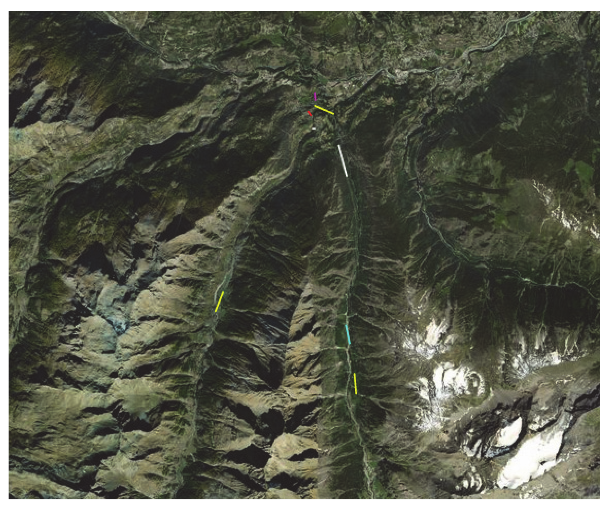Figure 3 reports the geolocalization of the critical components, i.e., the components with the highest failure probability. It is worth observing that all the damaged lines are MV lines with conductors with 35 mm² or 70 mm² cross sections.

Table 4. List of critical components with the relevant failure probabilities over 10 min, case A1.

ID			Failure Probability	Damaged Subcomponent
D533311	-	D543311:	0.86835	Conductor
D162311	-	D192311:	0.68913	Conductor
D573311	-	D583311:	0.56858	Conductor
D733311	-	D753311:	0.4632	Conductor
D332311	-	D352311:	0.4506	Conductor
D713311	-	D723311:	0.38509	Conductor
D222311	-	D232311:	0.079871	Conductor
D633311	-	D643311:	0.055966	Conductor

reports the list of the critical components in detail with the relevant failure probability over the time interval of 10 min and the subcomponent of the line which determines the line failure.

It is worth noticing that in all the critical MV lines detected, the most vulnerable subcomponent is the phase conductor. This result is consistent with the maintenance experience of distribution operators.

Figure 4 indicates the actual mechanical tensions produced by the storm (blue dots) on the MV and HV lines of the T&D system with their relevant rated tensile strength (indicated with red squares).

After identifying the critical components, RELIEF generates the set of risky (multiple, also dependent) contingencies involving the critical components, by considering the ex-ante impact metrics equal to the number of outage-affected components (henceforth named “contingency order”) and assuming a minimum ex-ante risk threshold which can include also high order multiple contingencies with high impacts but low probabilities (this threshold is set to 10⁻¹⁰ after a try and error approach).

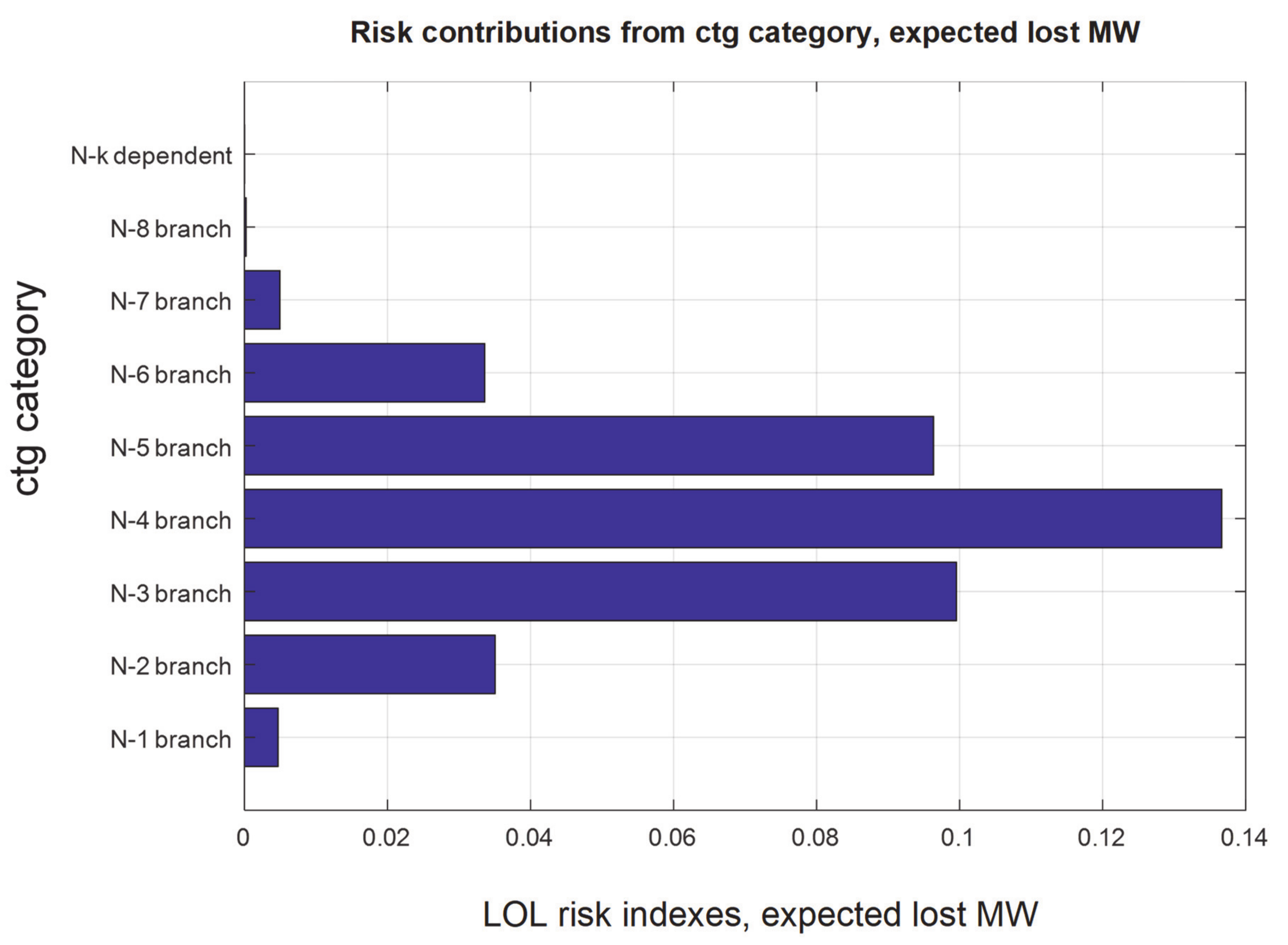
Figure 5 reports the contributions of the different contingency categories to the total risk of loss of load. In particular, the label “N-k branch” refers to the common mode N-k branch contingencies, while “N-k dependent” refers to multiple dependent contingencies (e.g., busbar contingencies). It is worth noting that the major contribution to the risk indicator comes from multiple common mode branch contingencies. Therefore, these contingencies cannot be ignored in resilience analyses. The total risk of loss of load is equal to 0.41 expected lost MW: 75% of total risk is due to N-2, N-3 and N-4 common mode branch contingencies.

3.3. Case M1.1: Reconductoring

This simulation assumes that all the critical branches with 35 mm² cross section are upgraded with 70 mm² cross-section conductors. Figure 6 reports the geolocalization of the critical branches.

Table 5. List of critical components with failure probabilities over 10 min, case M1.1.

ID			Failure Probability	Damaged Subcomponent
D733311	-	D753311:	0.4632	Conductor
D713311	-	D723311:	0.38509	Conductor
D633311	-	D643311:	0.055966	Conductor
D162311	-	D182311:	0.055026	Conductor
D603311	-	D613311:	0.026015	Power supports
D242311	-	D252311:	0.025488	Conductor
D643311	-	D663311:	0.02514	Conductor

reports the list of critical components. It can be noticed that there is a reduction in the number of critical components, as well as a decrease of the probability of failure due to wet snow induced stress.

Figure 7a compares the contributions to the total loss of load risk indicator between cases A1 and M1.1. It is worth noticing that the total LOL (Loss Of Load) risk passes from 0.41 expected lost MW in case A1 to 0.16 in case M1.1, showing a 61% reduction. This allows to quantify the benefits to resilience brought by the reconductoring measure. In particular, the major contribution comes from N-2 branch contingencies. Additionally, Figure 7b shows a quite clear trend: the higher the contingency order of multiple branch contingencies, the higher the median impact provoked in terms of loss of load.

3.4. Case A2: Severe Wet Snow Storm

This simulation considers a more severe wet snow storm with respect to the one described in case A1: in particular, the precipitation rate is still 2 mm/h with low wind speed peaks but the accumulated snow precipitation is set to 80 mm instead of 65 mm. The consequence consists of larger wet snow sleeves on the conductors and shield wires, thus larger mechanical stresses on all the subcomponents of the MV and HV OHLs.

Figure 8 reports the geolocalization of the critical components.

Table 6. List of critical components with their failure probabilities over 10 min, case A2.

	LINE ID		Failure Probability	Damaged Component
D332311	-	D352311:	0.99999	Conductor
D533311	-	D543311:	0.99998	Conductor
D573311	-	D583311:	0.99997	Conductor
D733311	-	D753311:	0.99996	Conductor
D713311	-	D723311:	0.99989	Conductor
D162311	-	D192311:	0.99666	Conductor
V091111	-	V201111:	0.96916	Shield
D773311	-	D783311:	0.92208	Conductor
V101111	-	V051131:	0.88755	Shield
D633311	-	D643311:	0.88521	Conductor
D412311	-	D422311:	0.8701	Conductor
V071111	-	V081111:	0.83787	Shield
V071111	-	V171111:	0.80166	Shield
D643311	-	D663311:	0.77317	Conductor
V191111	-	V171111:	0.73782	Shield
D883311	-	D893311:	0.71867	Conductor
D603311	-	D613311:	0.7069	tower supports
D853311	-	D863311:	0.67928	Conductor
D422311	-	D432311:	0.66223	Conductor
D673311	-	D693311:	0.65822	Conductor
D863311	-	D883311:	0.65028	Conductor
D222311	-	D232311:	0.64161	Conductor
V091111	-	V051131:	0.60362	Shield
V191111	-	V201111:	0.59542	Shield
D162311	-	D182311:	0.59466	Conductor
V051311	-	D072311:	0.48493	Conductor
D162311	-	D172311:	0.48129	Conductor
D392311	-	D402311:	0.44766	Conductor
V121211	-	V051211:	0.44613	Conductor
D893311	-	D903311:	0.43029	Conductor
D242311	-	D252311:	0.34717	Conductor
D833311	-	D843311:	0.28585	Conductor
D733311	-	D773311:	0.27145	Conductor
V151211	-	V161211:	0.25849	Conductor
V131211	-	V051211:	0.25262	Conductor
D663311	-	D673311:	0.24607	Conductor
V051322	-	D092311:	0.18891	Conductor
D382311	-	D392311:	0.18506	Conductor
D793311	-	D803311:	0.18033	Conductor
D402311	-	D412311:	0.1718	Conductor
D753311	-	D763311:	0.14452	Conductor
V141211	-	V171211:	0.11793	Conductor
V211211	-	V221211:	0.10208	Conductor

reports the complete list of critical components. It is worth noting that both MV and HV branches are included in the list. The most vulnerable subcomponents for MV lines are the phase conductors, which is consistent with DN operators’ operational experience. Moreover, for such large wet snow sleeves, HV lines also show large failure probabilities especially due to damages to shield wires (see for example lines V09-V20 and V10-V05). The TSO’s operational experience indicates that the conductors are in fact the least vulnerable subcomponents, while supports and shield wires are more subject to mechanical damages due to wet snow loads. These feedbacks from DSOs and TSOs grid operational experience confirm the soundness of the proposed physics-based analytical models for component vulnerability.

Moreover, among MV branches all 35 and 70 mm² show significant failure probabilities, while MV branches with ACSR conductors with 150 mm² cross-section do not appear in the list of critical components due to the fact that they have a very low initial tension (9.3%) which improves their ability to withstand heavy snow loads.

3.5. Case M2.1: Optimal Reconfiguration during Severe Storm

This scenario considers the N-2 outage of two critical branches connecting MV nodes D41-D42 and D16-D19 in the A2 base case, which causes the loss of supply of many customers connected to the Rhemes Valley feeder.

Table 7. Performance indicators for different counterfeed configurations in case of the outage of branches D41-D42 and D16-D19.

Configuration	% of Restored Load	Mv [p.u.]	Plosses [MW]
0  0  1	65.81	0.9956	0.0116
0  1  0	48.29	0.9987	0.0087
0  1  1	65.81	0.9956	0.0116
1  0  0	82.48	0.9971	0.012
1  0  1	100	0.9956	0.0149
1  1  0	82.48	0.9975	0.0109

compares some performance indexes (percentage of restored load, post contingency minimum voltage and active power losses) for the switching configurations with one or two switching on the three available counterfeeds. The “configuration” column reports the status of the three counterfeeds: 1 means “closed” while 0 means “open”.

Two main remarks can be derived:

• In the present case, there is no “one switching” reconfiguration of a counterfeed (k = 1) which allows to restore all the unsupplied load.
• After checking all the reconfigurations of two counterfeeds (k = 2), only one of these reconfigurations, specifically X_D63-D26 = 1, X_D26-D31 = 0 and X_D12-D46 = 1 (1 = “closed”, 0 = “open”), allows to restore all the unsupplied load with a minimum number of maneuvers, while preserving the radiality of the post-contingency network topology.

3.6. Case A3: Tree Falls Due to High Wind Speeds

This simulation assumes that the same area under study is affected by the severe weather conditions which occurred in the north of Italy in February 2015. As reported in Section 3.1 the wind speeds and wet snow precipitation rates correspond to the maximum values forecasted on the occasion of this severe real event. Strong wind has both direct effects (direct actions) and indirect effects (falling trees) on OHL subcomponents. The methodology is able to simulate both effects. In particular, considering the limit of wind speed for OHL design (130 km/h), the major source of damage is due to the fall of trees induced by strong winds.

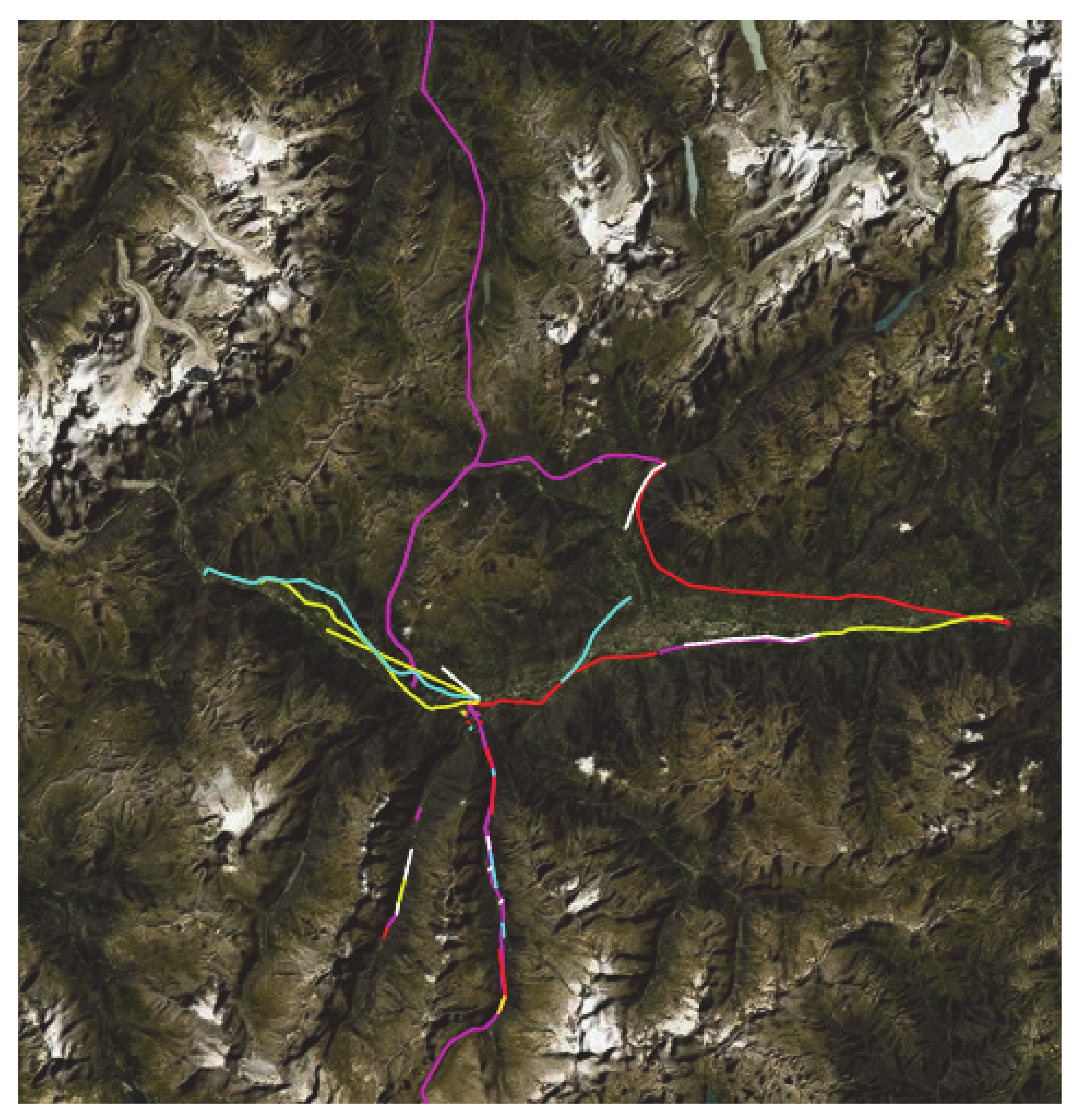
Figure 9 reports the geolocalization of the critical components for tree falls and the localization of the areas covered by tall trees according to the CORINE database [25].

The set of critical components is reported in

Table 8. List of critical components with their failure probabilities over 10 min, case A3.

Line ID			Failure Probability
D853311	-	D863311:	0.88837
D863311	-	D883311:	0.86207
D903311	-	D913311:	0.79399
D883311	-	D893311:	0.64361
D893311	-	D903311:	0.51418
D843311	-	D853311:	0.31828

.

It is worth noticing that all the lines with a high probability of failure due to tree falls belong to MV feeders, because of the smaller dimensions of the towers with respect to HV lines. The criticality of the branches in the southern part of the Valsavarenche feeder is confirmed by the DSO resilience plan [34] where the DSO reports relatively low resilience indexes and low return periods of outage (due to the dominant threat of “tree fall”) for the MV/LV substations (e.g., Degioz) connected to the last part of the above-mentioned feeder. This fact suggests a good matching between the resilience assessment tool outcomes and the DSO feedbacks from the field.

Again, the tool identifies the set of risky contingencies involving those critical components. Figure 10 reports the contributions to the total risk of loss of load on the basis of the order and type of contingencies. The total LOL risk is equal to 0.51 expected lost MW’s.

3.7. Case M3.1: 30% Enlargement of the ROW

The 30% enlargement of the ROW for MV lines does not provide any benefits to resilience, because according to the indications of the Italian standard CEI 11.4 the ROW is around 8–10 m for 15 kV lines (which means around 5 m per side). Given the mean height of the trees (i.e., 20 m) outside the ROW and the relatively low height of the MV line supports, the 30% enlargement does not avoid the interception of the line by the falling tree. On the other side, larger increments of the ROW would not be permitted by actual legislation, thus they are not realistic. The simulation carried out confirms the same set of critical components with the same failure probabilities.

The ROW enlargement is effective when the line support heights are comparable with the height of the trees outside the ROW, i.e., in case of HV lines exposed to interfering vegetation.

3.8. Case M3.2: Tree Height Trimming

In this case, it is assumed that a 5 m trimming is applied to the trees outside the ROW of the MV critical lines. The measure is effective; in fact, its implementation brings to the absence of critical components and carries a negligible risk of loss of load due to tree falls.

3.9. Case M3.3: Introduction of a New Counterfeed

This simulation considers the construction of a new counterfeed between nodes 48 and 91. The same situation as in case A3 is simulated but the response of DN also accounts for the availability of the new counterfeed.

Figure 11 compares the contributions to the total LOL risk for the present case M3.3 and base case A3. It can be noticed that the LOL risk passes from 0.51 in case A3 to 0.27 expected lost MW in case M3.3, showing a 47% reduction. This also justifies the choice of building the counterfeed which has been proposed in the DN operator resilience plan [34] to counteract faults in the area of nodes 84–90.

4. Discussion

A major condition for the applicability of the proposed resilience assessment and enhancement methodology discussed in the present paper consists of the verification of the analytical physics-inspired models for component vulnerability to the modelled threats. Given the low number of failure events available from operators’ recordings, it is hard to validate such models against failure statistics. However, several elements can be mentioned to support the capabilities of the developed vulnerability analytical models, at least with reference to the specific threats (wet snow and tree falls):

• With reference to wet snow events, in [14] the authors have applied the tool in the operational planning mode in order to anticipate potential critical lines due to mechanical damages for wet snow and wind loads during a real wet snow storm, which occurred in the north of Italy on 5–7 February 2015 on the basis of the weather forecasts produced on Feb 4. The simulations have shown a good matching between the list (updated hour by hour) concerning the OHLs with the highest failure probabilities and the set of OHLs which actually failed during the Feb 2015 event. Moreover, simulations of case A2 in the present paper also indicate that the most vulnerable subcomponent of MV (HV) OHLs is the conductor (cross-arms and support), which is confirmed by DSOs’ and TSO’s operational experience.
• As far as tree falls are concerned, in [22] the authors show that a typical value of wind speed which provokes the failure of OHL spans for indirect effects (i.e., interfering vegetation) with a not negligible (>10%) failure probability is around 70 km/h: the comparison of this threshold with the wind speed values recorded during some past events in the Italian grid (e.g., Vaia storm in 2018) confirms the soundness of the threshold evaluated with the analytical model. Moreover, as described in case M3, the combination of the CORINE database with the developed OHL vulnerability models allows to identify critical branches due to tree falls in the grid (last part of the Valsavarenche feeder).

The above-mentioned aspects confirm the capabilities of the proposed vulnerability models, which are essential conditions to assure the applicability of the results (failure probability of components, thus the probability of multiple contingencies in the grid).

The reported simulation cases demonstrate the ability of the tool to quantify not only the resilience of the integrated transmission and distribution system in case of an extreme event, but also the risk reduction of an unsupplied load which can be achieved via each of the simulated countermeasures. In this regard,

Table 9. Summary of resilience assessment results: LOL risk indicators before and after measure deployment, base cases A1, A3.

Case ID	Threat Scenario	Measure	LOL Risk before Measure Deployment [Expected Lost MW]	LOL Risk after Measure Deployment [Expected Lost MW]	Technical Benefit, Δ LOL Risk [Expected Lost MW]
A1	S1	Anticipation	0.41	-	-
A3	W1 + T	Anticipation	0.51	-	-
M1.1	S1	Reconductoring	0.41	0.16	+0.25
M3.1	W1 + T	30% enlarge ROW	0.51	0.51	0
M3.2	W1 + T	Height trimming	0.51	0	+0.51
M3.3	W1 + T	Adding a new counterfeed	0.51	0.27	+0.24

summarizes the LOL risk indicators for the resilience assessment of simulation cases A1 and A3, also highlighting the benefit of the applied countermeasures measured as the difference between the LOL risk indicator before and after the countermeasure deployment.

As far as severe wet snow storms in threat scenario S2 are concerned, the base case A2 is characterized by very severe multiple N-k branch contingencies affecting both transmission and distribution infrastructure. The active countermeasure simulated in case M2.1 allows to rapidly restore the whole load of DN for a specific low order N-k contingency, bringing a benefit to resilience in terms of reduction of the energy not supplied to MV/LV customers.

5. Conclusions

This paper has presented a comprehensive risk-based methodology and tool to assess and enhance the resilience of T&D systems subject to different threats. Simulations, performed on a detailed model of a real-world MV grid (i.e., two MV feeders in the Deval network in Aosta Valley) integrated with the surrounding HV/EHV grid, have demonstrated the main capabilities of the approach, i.e., its ability to simulate different threats, and the relevant response of the MV/HV grid, its flexibility to model the detailed vulnerability curves of both MV and HV grid components, and its ability to quantify the benefits of some resilience boosting measures (e.g., tree height trimming, reconductoring, optimal redispatching), in terms of reduction of loss of load risk, in case of threats with different severities. Performed simulations have confirmed the good agreement of the analytical models for component vulnerability with the operators’ feedback from the field.

Though the described examples focus on wet snow events and tree falls due to strong winds, the methodology can simulate a wide set of natural threats thanks to its general modeling framework, and it may represent a useful tool for resilience-oriented planning and operational planning. Even though the application cases refer to a specific DN (in Aosta Valley), the methodology is general and can be applied to any DN, provided that enough data are available to characterize the vulnerability of DN components to the specific threat under study. Further works will consist of a refinement of the modeling of the DN response to disturbances by including DG and storage. Modeling these devices will allow to enlarge the set of modelled mitigation measures.