Article

Trefftz Method of Solving a 1D Coupled Thermoelasticity Problem for One- and Two-Layered Media

Faculty of Management and Computer Modeling, Kielce University of Technology, 25-314 Kielce, Poland
*
Author to whom correspondence should be addressed.
Energies 2021, 14(12), 3637; https://doi.org/10.3390/en14123637
Submission received: 27 April 2021 / Revised: 9 June 2021 / Accepted: 15 June 2021 / Published: 18 June 2021
(This article belongs to the Special Issue Novel Numerical Methods in Heat and Mass Transfer)

Abstract

:
This paper discusses a 1D one-dimensional mathematical model for the thermoelasticity problem in a two-layer plate. Basic equations in dimensionless form contain both temperature and displacement. General solutions of homogeneous equations (displacement and temperature equations) are assumed to be a linear combination of Trefftz functions. Particular solutions of these equations are then expressed with appropriately constructed sums of derivatives of general solutions. Next, the inverse operators to those appearing in homogeneous equations are defined and applied to the right-hand sides of inhomogeneous equations. Thus, two systems of functions are obtained, satisfying strictly a fully coupled system of equations. To determine the unknown coefficients of these linear combinations, a functional is constructed that describes the error of meeting the initial and boundary conditions by approximate solutions. The minimization of the functional leads to an approximate solution to the problem under consideration. The solutions for one layer and for a two-layer plate are graphically presented and analyzed, illustrating the possible application of the method. Our results show that increasing the number of Trefftz functions leads to the reduction of differences between successive approximations.

1. Introduction

The multilayered materials have several unique characteristics that are frequently required and essential in structural design problems. To design an efficient composite structure, a detailed analysis must be carried out to check the stresses at the layer interfaces, where high local stresses may occur.
Various approaches and methods have been presented in the literature for the stress analysis of a multilayered medium. The authors of [1,2] presented the transfer matrix method for the isothermal elasticity problem that has been developed. In the paper [3] this approach has been extended to thermoelasticity problems. The authors of [4] employ the flexibility and stiffness matrix methods. To obtain the complete solution of the entire layered medium, this method has also been adopted by the authors of [5]. A transfer matrix formulation has been developed by the authors of [6] for longitudinal wave component propagation in both continuum and layered structures. The authors of [7] coupled thermoelastic problems for multilayered spheres are considered. Using the Laplace transform with respect to time, the general solutions of the governing equations are obtained in the transform domain. The solution is obtained using the matrix similarity transformation and inverse Laplace transform. The behavior of thermoelastic waves at the interface of layered medium and distributions of these waves through the domain is examined by applying the direct finite element method by the authors of [8]. The authors of [9] discuss the thermoelastic effects in the deformation of plates with arbitrary changing elastic parameters and temperature through-thickness. Using the semi-inverse method, a simple analytic solution is obtained for a thermoelastic problem of a nonhomogeneous plate with arbitrary contour. An analysis of displacements and stresses of FGM thick spherical pressure vessels with exponential varying material properties using the semi-analytical solution has been considered by the authors of [10]. In the paper [11] coupled thermoelasticity problems for a “coating-substrate” system are solved with the use made of the variational principle of coupled thermoelasticity in the Laplace transforms space and FEM. The transform inversion is realized according to the Durbin method [12]. The authors of [13] show that the exact solution for the temperature field has been obtained by separating variables and splitting the problem into two parts homogeneous transient and nonhomogeneous steady state. The set of equations obtained are solved using the rigorous applications of analytic techniques with the help of the eigen value expansion method. However, the thermoelastic response is studied in the context of uncoupled thermoelasticity. The authors of [14] study the mechanical behavior of two linear isotropic thermoelastic solids, bonded together by a thin layer, constituting a linear isotropic thermoelastic material, using an asymptotic analysis based on a finite element approach.
This work aims to obtain an approximate solution for predicting the temperature, displacement, and stress fields inside one- and two-layered thermoelastic media based on the coupled thermoelasticity equations. General solutions of homogeneous equations (displacement and temperature equations) are assumed to be a linear combination of Trefftz functions (T-functions). Particular solutions of these equations are then expressed by appropriately constructed sums of derivatives of general solutions, which is a novelty in solving the coupled equations. Then, the inverse operators to those appearing in homogeneous equations are defined. Applying them to the right-hand sides of the equations makes it possible to obtain such a form of solutions that can be used to determine the coefficients for T-functions.
The Trefftz method is widely described in many papers and monographs, and articles [15,16,17,18,19,20,21,22,23,24]. The T-functions for a linear partial differential equation usually can be obtained using the method of variables separation. Expanding the solution(s), called generating function(s), into power series with respect to the parameter(s) resulting from the method of variable separation, one arrives at the T-functions. In 2000, two new methods of deriving the T-functions were published. The one based on expanding function in the Taylor series is particularly simple and effective; the second is based on the so-called inverse operators [25,26,27]. To determine the unknown coefficients of these linear combinations, a functional is constructed that describes the error of meeting the initial and boundary conditions by approximate solutions. The minimization of the functional leads to an approximate solution to the problem under consideration.

2. Basic Equations

2.1. Heat Conduction Equation

Consider a perfectly conducting elastic infinite isotropic homogeneous medium without any heat sources or body forces. The relationship between the heat flux vector and the thermal disturbance in the thermal wave model is described as,
q = k T
Here q , [W/m2], is the heat flux, k , [W/(mK)] is the thermal conductivity, and T, [K], describes the temperature. When combined with the law of energy conservation for heat flux in the classical thermoelasticity,
q + Q = ρ c T t + γ T 0 u t
where Q, [W/m3] represents the internal source of heat in a material with density ρ , [kg/m3], c, [J/(kg K)], is the specific heat of the material, γ = ( 3 λ + 2 μ ) α T , α T   –coefficient of thermal expansion, [1/K], λ, μ are Lames constants, [kg/(ms2)], T 0 is the reference temperature, [K] and t, [s], stands for time. Hence, neglecting the internal heat source, the heat equation takes the form,
( k T ) =   t ( ρ c T + γ T 0 u )
with θ = T T 0 , ( k T ) = ( k θ , i ) , i and e u u i , i one obtains
( k θ , i ) , i =   t ( ρ c θ + γ T 0 u i , i )
( ) , i denotes differentiation with respect to the Cartesian coordinate x i ,   i = 1 , 2 , 3 and u i ,   i = 1 , 2 , 3 , are the components of the displacement vector. The thermal conductivity, k, will be considered as a constant. Finally, the heat equation takes the form,
[ Δ 1 a   t ] θ = γ T 0 k e t
with a = k ρ c , [m2/s], standing for thermal diffusivity.

2.2. Equations of Motion and Constitutive Equations

The equations of motion have the form,
ρ 2 u i t 2 = ( λ + μ ) 2 u j x i x j + μ 2 u i x j 2 γ θ , i ,   i = 1 , 2 , 3
Define components of strain tensor as follows:
ε i , j = 1 2 ( u i , j + u j , i ) ,             i = 1 , 2 , 3
Then the constitutive equations take the form,
σ i j = 2 μ ε i j + ( λ ε k k γ θ ) δ i j
σ i j are the components of stress tensor and δ i j is the Kronecker’s symbol. Moreover, ε k k e = ε 11 + ε 22 + ε 33 is dilatation.

3. Formulation of the Problem

The coordinate system is so chosen that the x-axis is taken perpendicularly to the considered layers, and the y- and z-axes in parallel (Figure 1). Assume that the y-axis is the symmetry axis of a layer above and below the y axis with the same boundary and initial conditions. Then, for x = 0, the temperature and displacement conditions will follow the assumed symmetry. In further considerations, the layers will be numbered as 1 and 2.
The problem is described by a system of two coupled equations:
[ 2 x 2 1 a   t ] θ = γ T 0 k 0 e   t
( ρ 2 t 2 ( λ + 2 μ ) 2 x 2 ) u = γ θ x
For 1D problem
σ 11 σ = ( λ + 2 μ ) ε 11 γ θ ;             ε 11 = u 1 , 1 u / x  
with u u 1 and e = u x . Moreover, σ σ 11 and the rest of the stress components are zero. Let us introduce the substitutions:
x = K x ,       u = K u ,         t = F t ,         q = M q ,         σ = R γ σ ,           θ = R θ , F = a K 2 [ 1 s ] ,     a = k ρ c   [ m 2 s ] ,     E = γ 2 T 0 a ( λ + 2 μ ) k   [ ] ,       γ = ( 3 λ + 2 μ ) α T   [ N m 2 K ] ,   K = 1 a λ + 2 μ ρ     [ 1 m ] ,       M = γ c ρ ( λ + 2 μ ) 3   [   m 2 W ] ,       R = γ λ + 2 μ     [ 1 K ]
Hence, Equations (8) and (9) take the form,
[ 2 x 2   t ] θ = E 2 u t x
( 2 t 2 2 x 2 ) u = θ x
The constitutive equation takes then the form,
σ = u x θ = e θ
By virtue of (1.1), in 1D, the relationship between the heat flux and the thermal disturbance can be expressed as,
q = k θ x   or   q = θ x
In further consideration, the primes are dropped for convenience.

3.1. Case I: One Layer

Consider Equations (11) and (12) and denote the dimensionless length l1 as l = K l 1 . The following dimensionless initial and boundary conditions are assumed:
  θ ( x , 0 ) = 0 ,    x [ 0 , l ]   u ( x , 0 ) = 0 ; u t ( x , 0 ) = 0    x [ 0 , l ]
θ   ( l , t ) = B C ( t ) , t ( 0 , t e n d ) u   x ( l , t ) B C ( t ) = 0 ,               t ( 0 , t e n d )
θ x ( 0 , t ) = 0         for       t ( 0 , t e n d ) u ( 0 , t ) = 0           for       t ( 0 , t e n d )
Here, the dimensionless length l 1 is denoted as l = l 1 a λ + 2 μ ρ and B C ( t ) stands for the boundary condition for θ   ( l , t ) (to be shown later).

3.2. Case II: Two Layers

Equations (11) and (12) hold for layer 1. The initial, boundary, and symmetry conditions have the same form in dimensional and dimensionless coordinates. The layers will be numbered as 1 and 2. The conditions on the border of the layers (i.e., for x = l 1 ) in dimensional form are as follows:
θ 1 ( l 1 , t ) = θ 2 ( l 1 , t ) ,                     t ( 0 , t e n d ) k 1 θ 1 x ( l 1 , t ) = k 2 θ 2 x ( l 1 , t )   ,         t ( 0 , t e n d ) u 1 ( l 1 , t ) = u 2 ( l 1 , t ) ,                 t ( 0 , t e n d ) ( ( λ + 2 μ ) 1 u 1   x γ 1 θ 1 ) ( l 1 , t ) = ( ( λ + 2 μ ) 2 u 2   x γ 2 θ 2 ) ( l 1 , t ) ,         t ( 0 , t e n d )
In dimensionless form, we can find l 1 l 1 ( 1 a λ + 2 μ ρ ) 1 = l 1 K 1 as an upper limit of layer 1 and l 1 l 1 K 2 as a lower limit of layer 2. Hence, l 1 = l 1 K 2 K 1 and x = x K 2 K 1 . The length l 2 can be expressed dimensionless by the thermophysical parameters of layer 1, l 2 = l 2 K 1 and of layer 2, l 2 = l 2 K 2 . Then, l 2 = l 2 K 2 K 1 . Moreover, because t = F 1 t ; then t = t F 2 F 1 . Thus, the conditions (18) in dimensionless form read (dropping the primes for convenience),
θ 1 ( l 1 , t ) = R 1 R 2 θ 2 ( l 1 K 2 K 1 , t F 2 F 1 ) θ 1 x ( l 1 , t ) = M 1 M 2 θ 2 x ( l 1 K 2 K 1 , t F 2 F 1 ) u 1 ( l 1 , t ) = K 1 K 2 u 2 ( l 1 K 2 K 1 , t F 2 F 1 ) u 1   x ( l 1 , t ) θ 1 ( l 1 , t ) = γ 2 R 1 γ 1 R 2 ( K 2 K 1 u 2   x ( l 1 K 2 K 1 , t F 2 F 1 ) θ 2 ( l 1 K 2 K 1 , t F 2 F 1 ) )
with R = γ ( λ + 2 μ ) , and t ( 0 , t e n d ) . Finally, (19) and all relations below refer to the dimensionless layer 1 coordinates.
Initial conditions for x [ 0 , l 1 ] (in layer 1) and x [ l 1 , l 1 + l 2 ] (in layer 2), i.e., x [ l 1 K 2 K 1 , ( l 1 + l 2 ) K 2 K 1 ] , take the form (with the primes dropped for convenience):
θ 1 ( x , 0 ) = 0   ,         x [ 0 , l 1 ]       θ 2 ( x , 0 ) = 0   ,         x [ l 1 K 2 K 1 , ( l 1 + l 2 ) K 2 K 1 ]      
u 1 ( x , 0 ) = 0   ,         u 1 t ( x , 0 ) = 0       x [ 0 , l 1 ]           u 2 ( x , 0 ) = 0   ,         u 2 t 2 ( x , 0 ) = 0 ,     x [ l 1 K 2 K 1 , ( l 1 + l 2 ) K 2 K 1 ]
Boundary conditions on the upper border of layer 2 in the dimensionless form read:
θ 2 ( ( l 1 + l 2 ) K 2 K 1 , t ) = B C ( t )   ,         t ( 0 , F 2 F 1 t e n d ) u 2   x ( ( l 1 + l 2 ) K 2 K 1 , t ) B C ( t ) = 0     ,     t ( 0 , F 2 F 1 t e n d )
with dimensionless t as for layer 1.
With the y axis anticipated as the symmetry axis, the following conditions are obtained for x = 0 :
θ 1 x ( 0 , t ) = 0         for   any   t ( 0 , t e n d )   u 1 ( 0 , t ) = 0   for   any   t ( 0 , t e n d )

4. Trefftz Functions and Inverse Operators

4.1. Trefftz Functions for Cases I and II

In order to find an approximate solution of the problems presented as Cases I and II, Trefftz functions (also called T-functions) for homogeneous Equations (11) and (12), i.e., for the equations
L U u ( 2 t 2 2 x 2 ) u = 0
L θ θ   ( 2 x 2   t ) θ = 0
have to be known, where L U 2 t 2 2 x 2 and L θ 2 x 2   t .
T-functions for Equation (24) can be easily derived from the harmonic functions putting in harmonic equation y = i t , i = 1 being the imaginary unit. Hence, one obtains,
F 1 n ( x , t ) = 1 n ! ( x + t ) n ,               F 2 n ( x , t ) = 1 n ! ( x t ) n
The T-functions F 1 n and F 2 n , n = 0 , 1 , , are then renumbered to form a string { F m } m = 0 , 1 , , M , M standing for number of functions. The approximate general solution of Equation (24), u b , is a linear combination of T-functions:
u b ( x , t ) = m = 0 M d m F m ( x , t )
T-functions for Equation (25) are known [18], and read,
g n ( x , t ) = k = 0 [ n 2 ] x n 2 k t k ( n 2 k ) ! k ! ,   n = 0 , 1 ,
The approximate general solution of Equation (25), θ b , is a linear combination of the T-functions:
θ b ( x , t ) = r = 0 R f r g r ( x , t )
d m ,   m = 0 , , M and f r ,   r = 0 , , R stand for coefficients of linear combinations (27) and (29) (to be calculated).

4.2. Inverse Operator for Operators (24) and (25)

The inverse operator L U 1 for Equation (24) can be determined as follows,
L U 1 ( x k t m ) = + x k t m + 2 k ( k 1 ) L U 1 1 ( x k 2 t m + 2 ) ( m + 2 ) ( m + 1 )
The inverse operator L θ 1 for Equation (25) can be determined as,
L θ 1 ( x k t m ) = x k t m + 1 + k ( k 1 ) L θ 2 1 ( x k 2 t m + 1 ) ( m + 1 )
It is easy to check that in both cases L L 1 ( x k t m ) = x k t m . For all inverse operators L 1 ( r k t m ) = 0 if k < 0 or m < 0 .
The T-functions and inverse operators for the case II are the same as for case I.

4.3. Solution of Nonhomogeneous System of Equations

The approximate solutions of Equations (11) and (12) will be expressed as a sum of the general solutions (27) and (29) and the particular solutions received by the operation of inverse operators, (30) and (31), on the right sides of Equations (11) and (12). Hence,
u a p ( x , t ) = u b ( x , t ) + u p ( x , t ) = m = 0 M d m I F m ( x , t ) L U 1 ( x n = 0 N f n g n ( x , t ) )
θ a p ( x , t ) = θ b ( x , t ) + θ p ( x , t ) = r = 0 R f r g r ( x , t ) + L θ 1 ( E 2 t x m = 0 M d m I F m ( x , t ) )
with u p and θ p standing for particular solutions of Equations (11) and (12). Of course, u b ( x , t ) = m = 0 M d m F m ( x , t ) and θ b ( x , t ) = r = 0 R f r g r ( x , t ) , i.e.,
u p ( x , t ) = L U 1 ( x θ ) = n = 0 N f n L U 1 ( x g n ( x , t ) )
θ p ( x , t ) = L θ 1 ( E 2 t x u ) = E m = 0 M d m I L θ 1 ( t x F m ( x , t ) )
Denote,
A = L U 1 ,   B = L θ 1 ,   C = E 2 t x ,   D = x
Then,
u p ( x , t ) = A ( D θ ) θ p ( x , t ) = B ( C u )
But,
u a p = u b + u p = u b + A ( D θ ) = u b + A ( D ( θ b + θ p ) ) = u b + A ( D ( θ b + B ( C u ) ) ) = = ( 1 + A D B C + A D B C A D B C + ) u b + A D ( 1 + B C A D + B C A D B C A D + ) θ b
Hence,
u a p = ( 1 + L U 1 ( x ) L θ 1 E 2 t x         + L U 1 ( x ) L θ 1 E 2 t x L U 1 ( x ) L θ 1 E 2 t x + ) u b         + L U 1 ( x ) ( 1 + L θ 1 E 2 t x L U 1 ( x )         + L θ 1 E 2 t x L U 1 ( x ) L θ 1 E 2 t x L U 1 ( x ) + ) θ b
Assuming that in the above presentation of u a p the number of products of the operators A, B, C, D is equal to n , the function u a p can be rewritten as,
u a p = m = 0 M d m k = 0 n [ L U 1 1 ( x ) L θ 1 1 E 2 t x ] k F m ( x , t ) + m = 0 N f m L U 1 1 ( x ) k = 0 n [ L θ 1 1 E 2 t x L U 1 1 ( x ) ] k g m ( x , t )
Similar operation applied to θ a p leads to the following result:
θ a p = θ b + θ p = θ b + B ( C u ) = θ b + B ( C ( u b + A ( D θ ) ) ) = = ( 1 + B C A D + B C A D B C A D + ) θ b + B C ( 1 + A D B C + A D B C A D B C + ) u b
Hence,
θ a p = m = 0 N f m k = 0 n [ L θ 1 E 2 t x L U 1 ( x ) ] k g m ( x , t ) + m = 0 M d m L θ 1 E 2 t x k = 0 n [ L U 1 ( x ) L θ 1 E 2 t x ] k F m ( x , t )
In the case of two layers, we do the same, remembering about different parameters for layers I and II.
It should be clearly emphasized that the solution is given by Formulas (36) and (37) fulfill exactly the system of Equations (11) and (12). For example, taking three Trefftz functions in Formula (27) and four Trefftz functions in Formula (29), we get,
θ a p = f 1 + f 2 x + f 3 ( 1 2 x 2 + t ) + f 4 ( 1 6 x 3 + x t ) + 1 2 f 4 E x t 2 + 1 2 f 3 E t 2 u a p = d 1 + d 2 ( x + t ) + d 3 ( x t ) 1 2 f 2 t 2 1 2 f 3 x t 2 f 4 ( 1 24 t 4 + 1 24 E t 4 + 1 4 x 2 t 2 + 1 6 t 3 ) .
It is easy to show that Functions (38) fulfill the system of Equations (11) and (12). The initial and boundary conditions are fulfilled approximately (see Section 5).

5. Objective Functionals

5.1. The Objective Functional for the Case I

The objective functional, having a form J ( x , t , { c n f n } , { d m } ) (in the case I denoted as J 1 ), which describes the mean square error of fulfilling the initial, the boundary, and the internal conditions, is defined as follows:
J x 1 = 0 l [ ( θ a p ( x , 0 ) ) 2 + ( u a p ( x , 0 ) ) 2 + ( u a p t ( x , 0 ) ) 2 ] d x   for   conds   ( 15 )
J 1 t 1 = 0 t e n d [ ( θ a p ( l , t ) B C ( t ) ) 2 + ( u   a p   x ( l , t ) B C ( t ) ) 2 ] d t   for   conds   ( 16 )
J 2 t 1 = 0 t e n d ( θ a p x ( 0 , t ) ) 2 + ( u a p ( 0 , t ) ) 2 d t   for   conds   ( 17 )
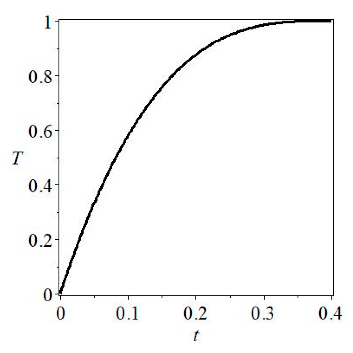
As B C ( t ) , we take for calculations,
B C ( t ) = 1000 64 ( t 4 10 ) 3 + 1
Finally, the objective functional J 1 reads,
J 1 ( x , t , { f n } , { d m } , ) = J 1 t I + J 2 t I + J x I
Figure 2 shows the boundary condition (39) for t ( 0 ,   0.4 ) .

5.2. The Objective Functional for the Case II

The objective functional J 2 ( x , t , { f n 1 } , { f n 2 } , { d m 1 } , { d m 2 } ) , which describes the mean square error of fulfilling the initial, the boundary, and the internal conditions, consists of the following functionals:
J 11 x 2 = 0 l 1 [ ( θ 1 a p ( x , 0 ) ) 2 + ( u 1 a p ( x , 0 ) ) 2 + ( u 1 a p t ( x , 0 ) ) 2 ] d x
for cond (20)1 and (21)1,
J 12 x 2 = l 1 K 2 K 1 ( l 1 + l 2 ) K 2 K 1 [ ( θ 2 a p ( x , 0 ) ) 2 + ( u 2 a p ( x , 0 ) ) 2 + ( u 2 a p t ( x , 0 ) ) 2 ] d x
for cond (20)2 and (21)2,
J 2 t 2 = 0 F 2 F 1 t e n d [ ( θ 2 a p ( ( l 1 + l 2 ) K 2 K 1 , t ) B C ( t ) ) 2 + ( u 2 a p   x ( ( l 1 + l 2 ) K 2 K 1 , t ) B C ( t ) ) 2 ] d t
for conds (22),
J 3 t θ 2 = 0 t e n d [ (   θ 1 a p ( l 1 , t ) R 1 R 2 θ 2 a p ( l 1 K 2 K 1 , t F 2 F 1 ) ) 2 + ( θ 1 a p x ( l 1 , t ) M 1 M 2 θ 2 a p x ( l 1 K 2 K 1 , t F 2 F 1 ) ) 2 ] d t
for conds (19)1 and 2,
J 3 t u 2 = 0 t e n d ( u 1 a p ( l 1 , t ) K 1 K 2 u 2 a p ( l 1 K 2 K 1 , t F 2 F 1 ) ) 2 d t
J 3 t σ 2 = 0 t e n d ( u 1 a p   x ( l 1 , t ) θ 1 a p ( l 1 , t ) γ 2 R 1 γ 1 R 2 ( K 2 K 1 u 2 a p   x θ 2 a p ) ( l 1 K 2 K 1 , t F 2 F 1 ) ) 2 d t
for conds (19)3 and 4,
J 4 t 2 = 0 t e n d ( θ 1 a p x ( 0 , t ) ) 2 + ( u 1 a p ( 0 , t ) ) 2 d t   for   conds   ( 23 )
Finally,
J 2 ( x , t , { f n I } , { f n I I } , { d m I } , { d m I I } ) = J 11 x 2 + J 12 x 2 + J 2 t 2 + J 3 t θ 2 + J 3 t u 2 + J 3 t σ 2 + J 4 t 2

6. Numerical Results and Discussion

For numerical computations, the physical constants of stainless steel and Lead Zirconate titanate (PZT-5A) [28], are considered as in Table 1. The computations were carried out for dimensionless length l 1 = 1 and l 2 = 0.1 the numerical values of the temperature, stress, and displacement are represented graphically. The lengths l 1 and l 2 are expressed dimensionless by the thermophysical parameters of layer 1.

6.1. Results for Case I

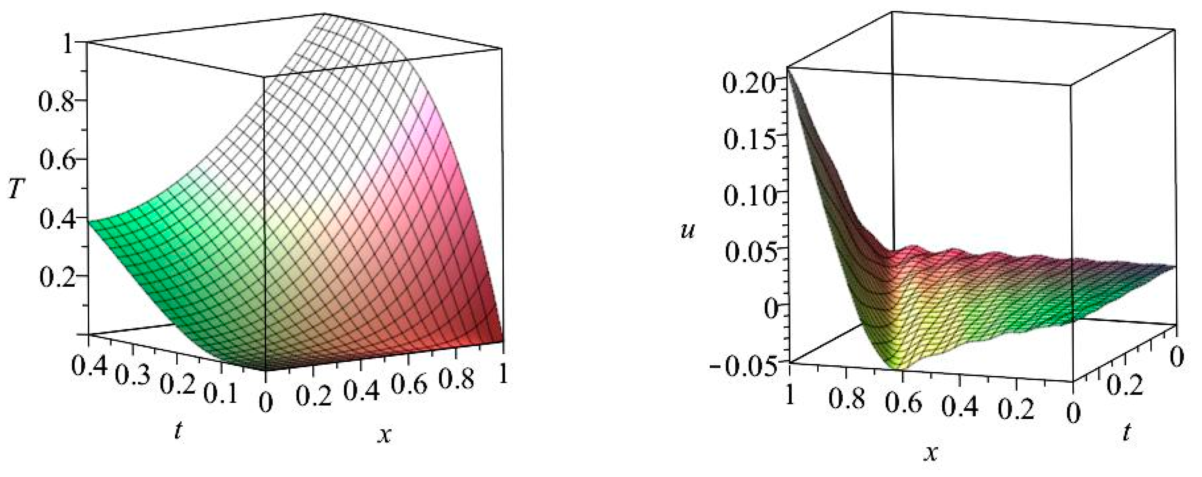
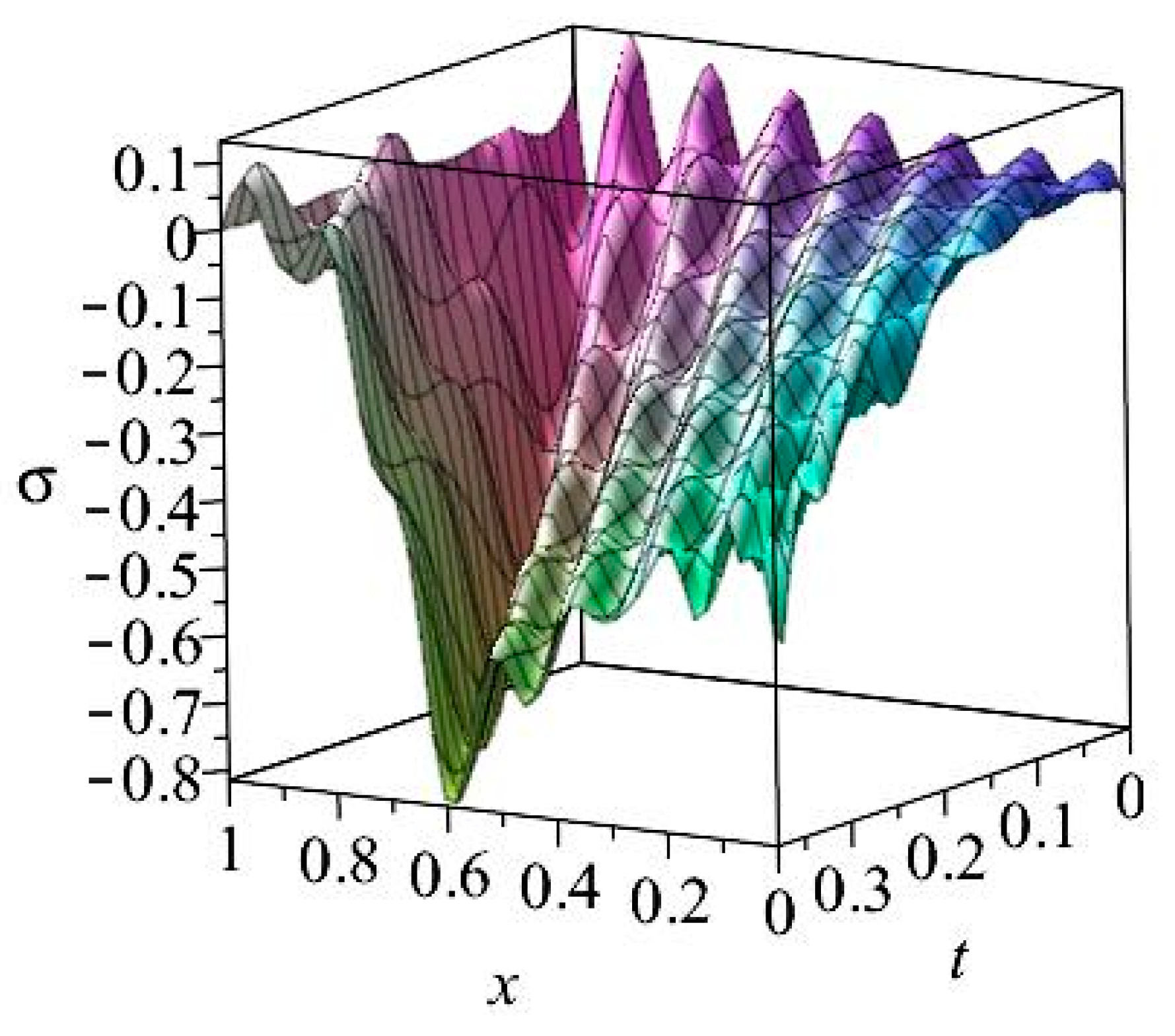
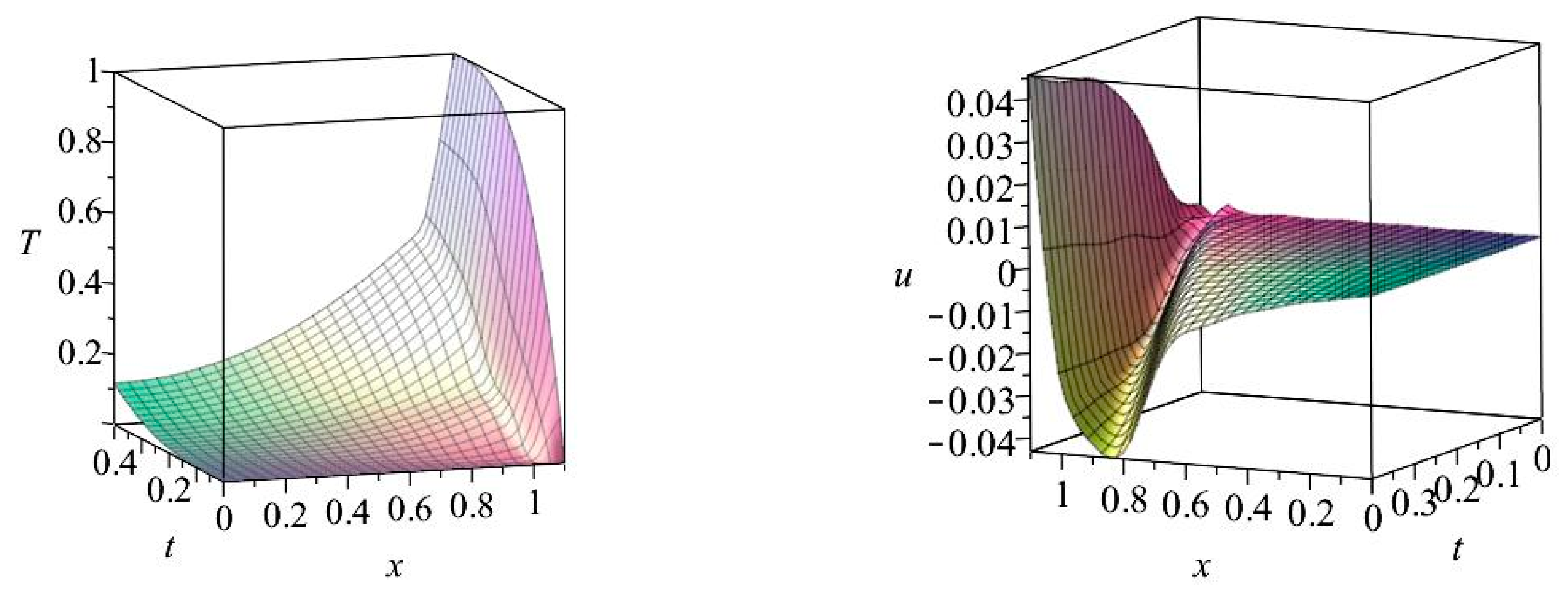
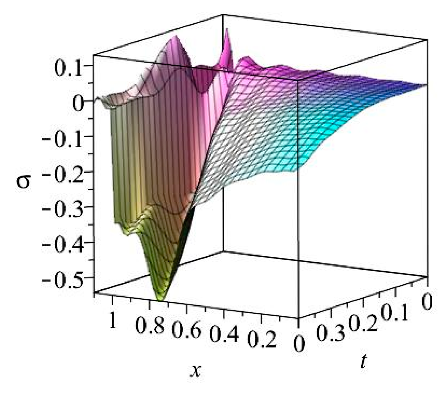
The calculations for one layer with dimensionless length l1 = 1 are shown in the graphs presented in Figure 3. They were performed with the approximation of the solutions by a 34-degree polynomial (34 T-functions for Equation (25) and 67 T-functions for Equation (24)).
In order to investigate whether the process of calculating temperature, displacement, and stress is convergent, the maximum norm has been examined,
z = max z Z | z |
for successive differences of solutions obtained for degree 10 (2) 34 (i.e., 10, 12, 14, …, 34) polynomials which approximate solutions. The maximum norm was investigated for differences in solutions in the space-time domain for z = ( x , t ) Z = ( 0 ,   1 ) × ( 0 ,   0.4 ) (Table 2) and for an approximation of the boundary condition for l 1 = 1 for t ( 0 ,   0.4 ) (Table 3).
The data presented in Table 2 and Table 3 show that the process of approximating solutions for temperature, displacement, and stress, as well as the process of approximating the boundary condition for temperature for l 1 = 1 are convergent.
Figure 3 shows that the plot for the stress field is waving strongly. This is due to the differentiation of displacements, cf. (13). The displacement field shows slight wavings; they strengthen for stresses. This is a characteristic feature of solutions described by a linear combination of polynomials. This phenomenon disappears as the number of polynomials increases. However, increasing the number of polynomials significantly increases computation time. Since the calculations were performed on a PC, this indicates the need to use a much faster computer. It is worth mentioning that the T-functions for each of the equations constitute a complete system of functions [18,27].

6.2. Results for Case II

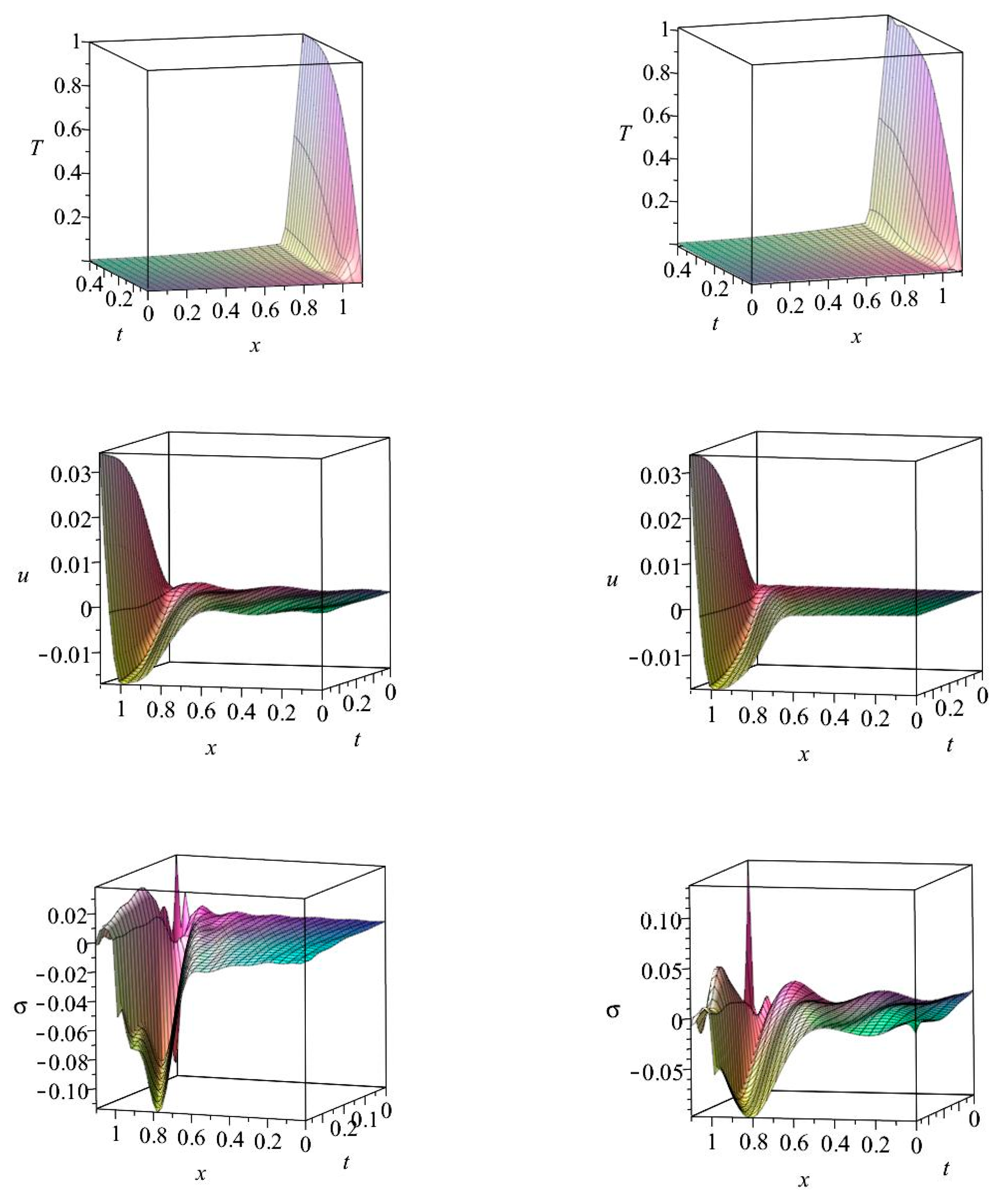
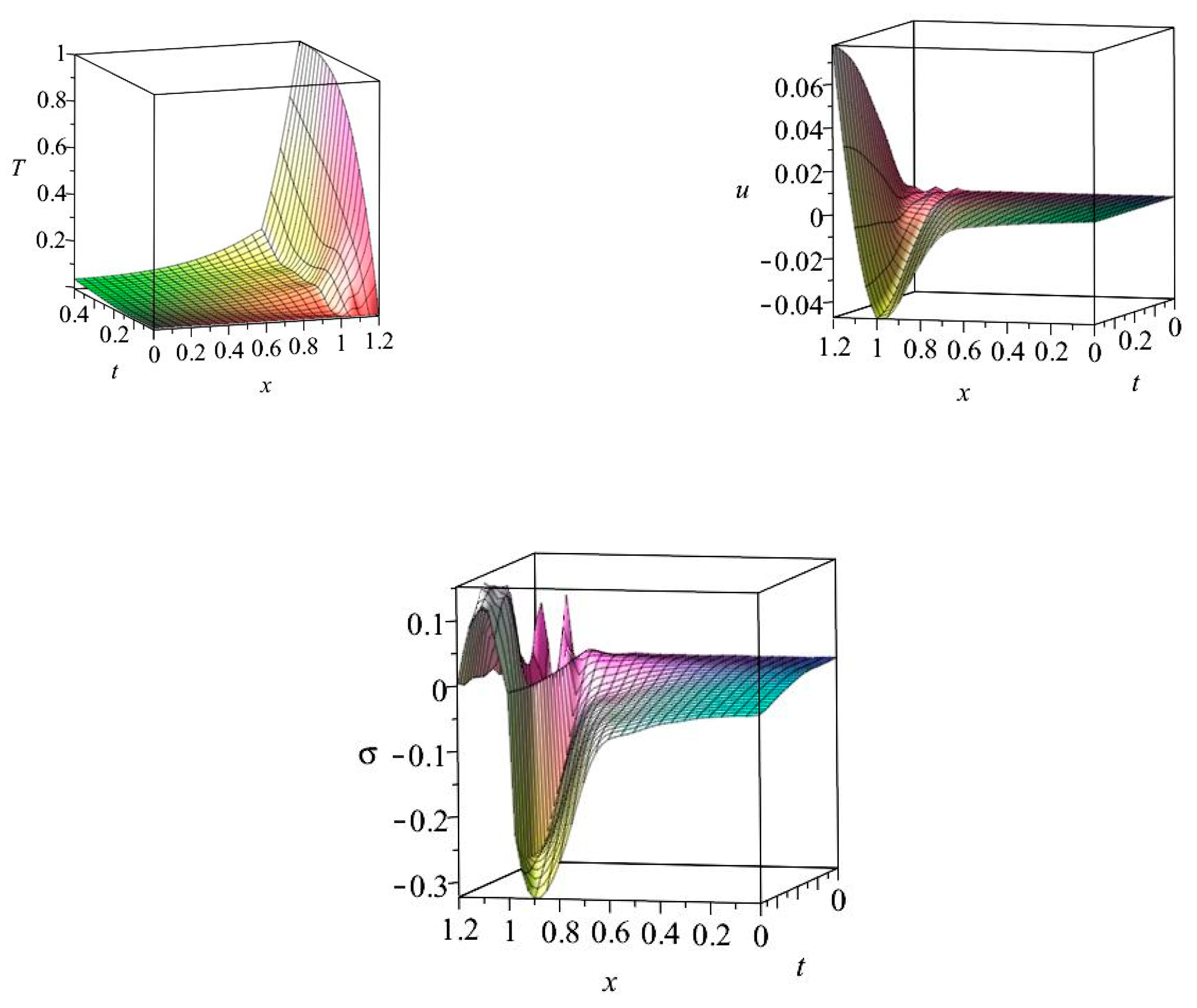
Calculations for two layers with dimensionless lengths l1 = 1, l2 = 0.1 are shown in the graphs in Figure 4. There are presented graphs for 11th and 25th degree polynomials. The comparison of the graphs shows how the degree of the used polynomial (combination of T-functions) affects the accuracy of the solution.
The graphs in Figure 4 show that in the case of temperature (top row), the number of polynomials slightly affects the shape of the graph. On the other hand, with higher degrees of the polynomial, both the displacement graphs (middle row), and stress graphs (bottom row) smooth out.
In order to investigate whether the process of calculating temperatures, displacements, and stresses in each of the two layers is convergent, the maximum norm was again tested for successive differences of solutions obtained for 9, 11, 13, …, 25 for layer 1 (for layer 2 it was 9, 13, 17, …, 25) T-functions for Equation (25) and a correspondingly doubled number of T-functions for Equation (24) in both layers. The maximum norm was investigated for the differences in solutions in the space-time domain for z = ( x , t ) Z = ( 0 ,   1 ) × ( 0 ,   0.4 ) . The data presented in Table 4 and Table 5 show that the process of approximating solutions for temperature, displacement, and stress in each layer separately are convergent processes.
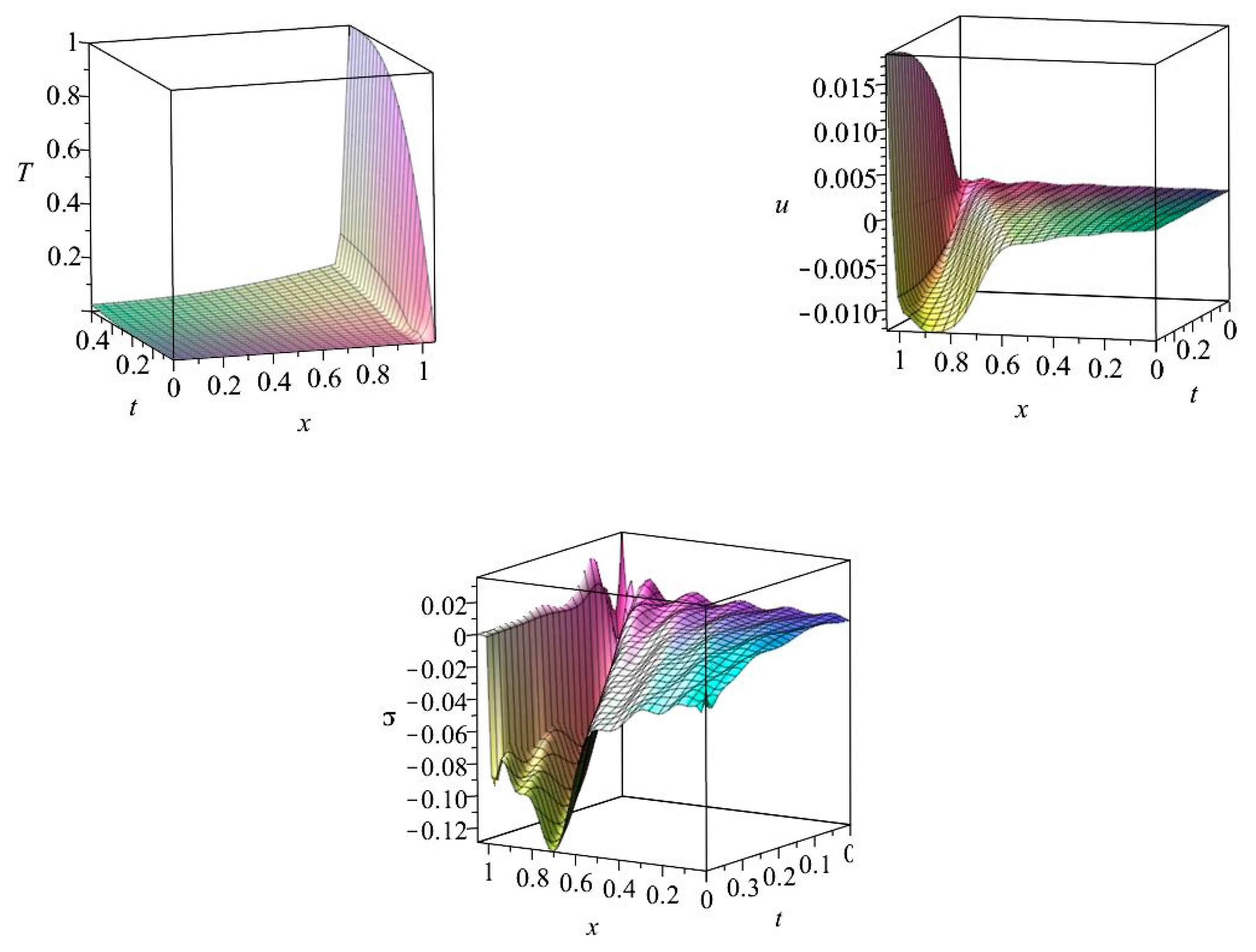
The influence of the thermal conductivity of layer 2 and its thickness on the distribution of temperatures, displacements, and stresses in the layers was also investigated. The results are presented in the graphs in Figure 5, Figure 6 and Figure 7.
The comparison of the temperature, displacement, and stress graphs in Figure 4 with the graphs in Figure 5 shows much higher temperature values in the first layer, resulting from the greater conductivity in the second layer, and higher values of displacements with reduced stress values.
Figure 6 shows a significant influence of the thickness of layer 2 and its thermal conductivity coefficient on the values of temperature and displacements in layer 2 at significantly reduced stresses in this layer. Figure 7 shows that reducing the thickness of layer 2 slightly increases the temperature in layer 1, slightly reduces the displacements on the outer edge of layer 1, and slightly disturbs the stresses.

7. Conclusions

The application of the Trefftz functions to the approximate solution of the thermoelastic problem in a single- and double-layered medium showed the effectiveness of the Trefftz method in connection with the method introduced in the article for determining particular solutions of coupled thermoelasticity equations. However, the solution procedure requires a powerful computer that will approximate solutions with high-order polynomials. The temperature and displacement fields in one and two layers could be obtained in a satisfactory form for a small number of T-functions (even for the solutions to be approximated by a 10-degree polynomial). The calculation of stresses requires a much higher degree of the approximating polynomial, due to the differentiation in Formula (13), which introduces significant undulations in the stress diagram. The applied method obtains an analytical solution with numerically determined coefficients at the Trefftz functions.
As composite materials are used on a larger scale, a rationale for research is the effect of sudden changes in their thermophysical properties [29,30]. The presented problem of thermo-structural analysis is part of this research area.
It should be emphasized that the approximate solution (in the form of a linear combination of the Trefftz function), which strictly fulfilled the fully coupled system of thermoelasticity equations is presented in the paper. It is probably the first time that such a solution has been obtained in this manner.

Author Contributions

Conceptualization, K.G. and A.M.; methodology, K.G. and A.M.; software, A.M.; validation, K.G. and A.M.; formal analysis, K.G. and A.M.; investigation, K.G. and A.M.; resources, K.G. and A.M.; data curation, K.G. and A.M.; writing—original draft preparation, K.G.; writing—review and editing, K.G. and A.M.; visualization, K.G. and A.M.; supervision, K.G. and A.M.; project administration, not applicable; funding acquisition, not applicable. All authors have read and agreed to the published version of the manuscript.

Funding

Kielce University of Technology.

Institutional Review Board Statement

Not applicable.

Informed Consent Statement

Not applicable.

Conflicts of Interest

The authors declare no conflict of interest.

References

  1. Bufler, H. Theory of Elasticity of a Multilayered Medium. J. Elast. 1971, 1, 125–143. [Google Scholar] [CrossRef]
  2. Bahar, L.Y. Transfer Matrix Approach to Layered Systems. J. Eng. Mech. Div. 1972, 98, 1159–1172. [Google Scholar] [CrossRef]
  3. Bahar, L.Y.; Hetnarski, R.B. Coupled Thermoelasticity of a Layered Medium. J. Therm. Stress. 1980, 3, 141–152. [Google Scholar] [CrossRef]
  4. Thangjitham, S.; Choi, H.J. Thermal Stresses in a Multilayered Anisotropic Medium. ASME J. Appl. Mech. 1991, 58, 1021–1027. [Google Scholar] [CrossRef]
  5. Chen, T.; Jang, H.; Tseng, A.A. Transient Thermal Stresses in a Multilayered Anisotropic Medium. ASME J. Appl. Mech. 1995, 117, 1067–1069. [Google Scholar] [CrossRef]
  6. Cetinkaya, C.; Li, C. Propagation and Localization of Longitudinal Thermoelastic Waves in Layered Structures. J. Vib. Acoust. 2000, 122, 263–271. [Google Scholar] [CrossRef]
  7. Lee, Z.-Y. Coupled Problem of Thermoelasticity for Multilayered Spheres with Time-Dependent Boundary Conditions. J. Mar. Sci. Tech. 2004, 12, 93–101. [Google Scholar]
  8. Hosseini Zad, S.K.; Komeili, A.; Eslami, M.R.; Fariborz, S. Classical and Generalized Coupled Thermoelasticity Analysis in One-Dimensional Layered Media. Arch. Appl. Mech. 2012, 82, 267–282. [Google Scholar] [CrossRef]
  9. Koo, J.; Valgur, J. Analysis of Thermoelastic Stresses in a Layered Plates. In Proceedings of the 6th International DAAAM Baltic Conference. Industrial Engineering, Tallinn, Estonia, 24–26 April 2008. [Google Scholar]
  10. Zamani Nejad, M.; Rastgoo, A.; Hadi, A. Effect of Exponentially-Varying Properties on Displacements and Stresses in Pressurized Functionally Graded Thick Spherical Shells with Using Iterative Technique. J. Solid Mech. 2014, 6, 366–377. [Google Scholar]
  11. Vatulyan, A.; Nesterov, S.; Nedin, R. Regarding some Thermoelastic Models of “Coating-Substrate” System Deformation. Contin. Mech. Thermodyn. 2020, 32, 1173–1186. [Google Scholar] [CrossRef]
  12. Durbin, F. Numerical Inversion of Laplace Transforms: An Efficient Improvement to Dubner and Abate’s Method. Comput. J. 1974, 17, 371–376. [Google Scholar] [CrossRef]
  13. Pawar, S.P.; Bikram, J.J.; Kedar, G.D. Thermoelastic Behaviour in a Multilayer Composite Hollow Sphere with Heat Source. J. Solid Mech. 2020, 12, 883–901. [Google Scholar] [CrossRef]
  14. Serpilli, M.; Dumont, S.; Rizzoni, R.; Lebon, F. Interface Models in Coupled Thermoelasticity. Technologies 2021, 9, 17. [Google Scholar] [CrossRef]
  15. Qin, Q.H. The Trefftz Finite and Boundary Element Method; WIT Press: Southampton, UK; Boston, MA, USA, 2000. [Google Scholar]
  16. Li, Z.C.; Lu, T.T.; Hu, H.Y.; Cheng, A. The Trefftz and Collocation Methods; WIT Press: Southampton, UK, 2008. [Google Scholar]
  17. Maciąg, A. Trefftz Functions for Some Direct and Inverse Problems of Mechanics; Kielce University of Technology Publishers: Kielce, Poland, 2009. (In Polish) [Google Scholar]
  18. Grysa, K. Trefftz Functions and Their Applications in Solving the Inverse Problems; Kielce University of Technology Publishers: Kielce, Poland, 2010. (In Polish) [Google Scholar]
  19. Maciąg, A. Trefftz Function for a Plate Vibration Problem. J. Theor. Appl. Mech. 2011, 49, 97–116. [Google Scholar]
  20. Grysa, K.; Maciąg, A. Solving Direct and Inverse Thermoelasticity Problems by Means of Trefftz Base Functions for Finite Element Method. J. Therm. Stress 2011, 34, 78–93. [Google Scholar] [CrossRef]
  21. Grysa, K.; Maciąg, A.; Adamczyk-Krasa, J. Trefftz Functions Applied to Direct and Inverse Non-Fourier Heat Conduction Problems. J. Heat Transf. 2014, 136, 091302. [Google Scholar] [CrossRef]
  22. Maciejewska, B.; Piasecka, M. An Application of the Non-Continuous Trefftz Method to the Determination of Heat Transfer Coefficient for Flow Boiling in a Minichannel. Heat Mass Transf. 2016, 53, 1211–1224. [Google Scholar] [CrossRef] [Green Version]
  23. Frackowiak, A.; Cialkowski, M. Application of Discrete Fourier Transform to Inverse Heat Conduction Problem Regularization. Int. J. Numer. Meth. Heat Fluid Flow 2018, 28, 239–253. [Google Scholar] [CrossRef]
  24. Grysa, K.; Maciąg, A. Identifying Heat Source Intensity in Treatment of Cancerous Tumor Using Therapy Based on Local Hyper-thermia—The Trefftz method approachs. J. Therm. Biol. 2019, 84, 16–25. [Google Scholar] [CrossRef]
  25. Ciałkowski, M.J. Trefftz Functions as Basic Functions of FEM in Application to Solution of Inverse Heat Conduction Problem. Comp. Ass. Mech. Eng. Sci. CAMES 2001, 8, 247–260. [Google Scholar]
  26. Cialkowski, M.J.; Frackowiak, A. Thermal and related functions used in solving certain problems of mechanics, Part I. Solving some differential equations with the use of inverse operator. In Modern Problems of Technics; University of Zielona Góra Publishers: Zielona Góra, Poland, 2003; Volume 3, pp. 7–70. [Google Scholar]
  27. Maciąg, A. The Usage of Wave Polynomials in Solving Direct and Inverse Problems for Two-Dimensional Wave Equation. Commun. Numer. Meth. Eng. 2011. [Google Scholar] [CrossRef]
  28. Sharma, J.N.; Pal, M.; Chand, D. Three-Dimensional Vibration Analysis of a Piezothermoelastic Cylindrical Panel. Int. J. Eng. Sci. 2004, 42, 1655–1673. [Google Scholar] [CrossRef]
  29. Abrate, S. Impact on Composite Structures; Cambridge University Press: Cambridge, MA, USA, 1998; p. 289. [Google Scholar]
  30. Sfarra, S.; López, F.; Sarasini, F.; Tirillò, J.; Ferrante, L.; Perilli, S.; Ibarra-Castanedo, C.; Paoletti, D.; Lampani, L.; Barbero, E.; et al. Analysis of damage in hybrid composites subjected to ballistic impacts: An integrated non-destructive approach. In Handbook of Composites from Renewable Materials; Scrivener Publishing: Beverly, MA, USA, 2017; Chapter 8; pp. 175–210. [Google Scholar] [CrossRef]
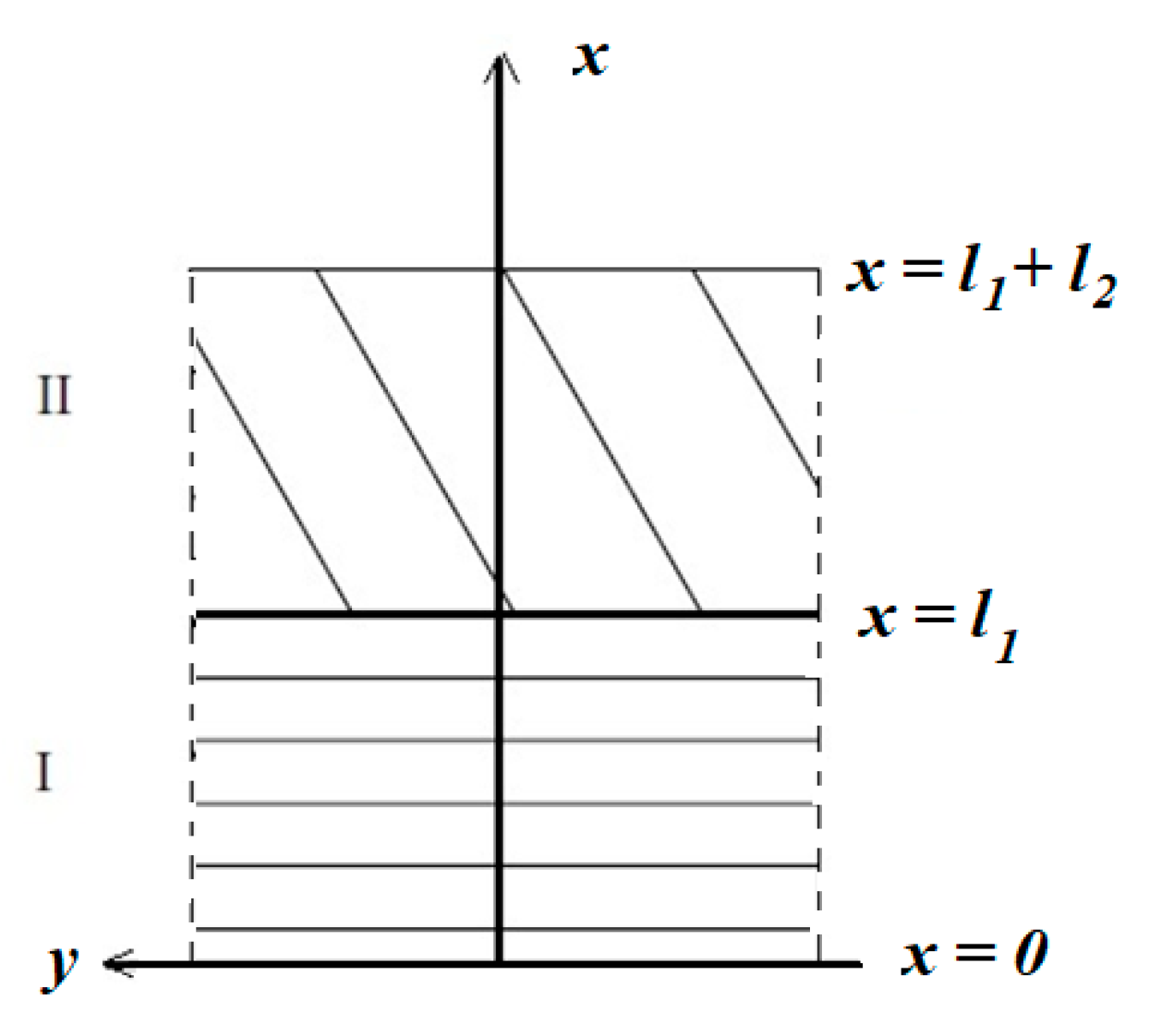
Figure 1. A layered medium.
Energies 14 03637 g001
Figure 2. Temperature boundary condition (Formula (39)).
Energies 14 03637 g002
Figure 3. Temperature field, T, displacements, u, and stresses, σ, in one layer.
Energies 14 03637 g003aEnergies 14 03637 g003b
Figure 4. Temperature (top row), displacement (middle row), and stress (bottom row) field for two layers. On the left—approximation by a 10th degree polynomial, on the right—by a 24th degree polynomial.
Energies 14 03637 g004
Figure 5. The thermal conductivity coefficient increased by four times for layer 2, the thickness of the layers remained unchanged.
Energies 14 03637 g005aEnergies 14 03637 g005b
Figure 6. The thermal conductivity coefficient increased by four times for thermal conductivity coefficient for layer 2, and two times for a greater thickness of layer 2.
Energies 14 03637 g006
Figure 7. The thermal conductivity coefficient for layer 2 as in Table 1, the thickness of layer 2 is two times smaller.
Energies 14 03637 g007
Table 1. The material properties.
The ParameterStainless SteelPZT-5A
ρ  [ kg / m 3 ]79707750
C [ m 2 / Ks 2 ]561420
T 0 [K]293293
k [ W / mK ]19.51.5
λ [ N / m 2 ]105.5 × 10 9 7.54 × 10 10
μ [ N / m 2 ]74 × 10 9 2.56 × 10 10
α T   [ K 1 ] 17.7 × 10 6 352 × 10 6
Table 2. The maximum norm for differences (upper row) for boundary condition BC and for temperature, displacement, and stress in the space-time domain.
12–1014–1216–1418–1620–1822–2024–2226–2428–2630–2832–3034–32
BC0.0120.0070.0060.0080.00650.00250.00450.0040.00120.0010.00150.0008
T0.0120.0070.0070.0080.00650.00250.00450.0040.00120.0010.00150.0008
U0.0250.0270.0090.0050.0060.0030.0030.0030.0030.0030.0020.002
σ0.40.50.20.30.140.080.110.10.110.150.070.07
Table 3. The maximum norm for the difference between the boundary condition BC for temperature for l 1 = 1 and its approximation.
N =10121416182022242628303234
BC—Tn0.0350.0280.0210.0150.0150.0110.0090.0090.0070.0060.0050.0040.0037
Table 4. The maximum norm for differences (upper row) for temperature, displacement, and stress in the space-time domain in layer 1.
11–913–1115–1317–1519–1721–1923–2125–23
T0.0710.0370.0110.010.0140.0050.0040.004
u0.00280.000950.00120.000220.00040.000190.000350.00025
σ0.080.0340.0350.0160.030.0130.0220.008
Table 5. The maximum norm for differences (upper row) for temperature, displacement, and stress in the space-time domain in layer 2.
13–917–1321–1725–21
T0.0850.0110.0150.0055
u0.00320.00110.000450.0004
σ0.110.0450.0350.02
Publisher’s Note: MDPI stays neutral with regard to jurisdictional claims in published maps and institutional affiliations.