Article

Forecasting of Day-Ahead Natural Gas Consumption Demand in Greece Using Adaptive Neuro-Fuzzy Inference System

by
Konstantinos Papageorgiou
1,*,
Elpiniki I. Papageorgiou
2,3,
Katarzyna Poczeta
4,
Dionysis Bochtis
3,* and
George Stamoulis
5
1
Department of Computer Science and Telecommunications, University of Thessaly, 35100 Lamia, Greece
2
Department of Energy Systems, Faculty of Technology, University of Thessaly-Geopolis, 41500 Larissa, Greece
3
Center for Research and Technology—Hellas (CERTH), Institute for Bio-economy and Agri-technology (iBO), 57001 Thessaloniki, Greece
4
Department of Information Systems, Kielce University of Technology, 25-314 Kielce, Poland
5
Department of Electrical and Computer Engineering, University of Thessaly, 38221 Volos, Greece
*
Authors to whom correspondence should be addressed.
Energies 2020, 13(9), 2317; https://doi.org/10.3390/en13092317
Submission received: 31 March 2020 / Revised: 3 May 2020 / Accepted: 4 May 2020 / Published: 7 May 2020
(This article belongs to the Special Issue Supply Chain Management for Bioenergy and Bioresources)

Abstract

:
(1) Background: Forecasting of energy consumption demand is a crucial task linked directly with the economy of every country all over the world. Accurate natural gas consumption forecasting allows policy makers to formulate natural gas supply planning and apply the right strategic policies in this direction. In order to develop a real accurate natural gas (NG) prediction model for Greece, we examine the application of neuro-fuzzy models, which have recently shown significant contribution in the energy domain. (2) Methods: The adaptive neuro-fuzzy inference system (ANFIS) is a flexible and easy to use modeling method in the area of soft computing, integrating both neural networks and fuzzy logic principles. The present study aims to develop a proper ANFIS architecture for time series modeling and prediction of day-ahead natural gas demand. (3) Results: An efficient and fast ANFIS architecture is built based on neuro-fuzzy exploration performance for energy demand prediction using historical data of natural gas consumption, achieving a high prediction accuracy. The best performing ANFIS method is also compared with other well-known artificial neural networks (ANNs), soft computing methods such as fuzzy cognitive map (FCM) and their hybrid combination architectures for natural gas prediction, reported in the literature, to further assess its prediction performance. The conducted analysis reveals that the mean absolute percentage error (MAPE) of the proposed ANFIS architecture results is less than 20% in almost all the examined Greek cities, outperforming ANNs, FCMs and their hybrid combination; and (4) Conclusions: The produced results reveal an improved prediction efficacy of the proposed ANFIS-based approach for the examined natural gas case study in Greece, thus providing a fast and efficient tool for utterly accurate predictions of future short-term natural gas demand.

Graphical Abstract

1. Introduction

The increasing technological advancements and the rapid global population growth have led to a remarkable increase in energy consumption all over the world and especially in the developed and developing countries. After all, energy consumption is an index of a society’s economical welfare and represents the economic development of a city or country [1]. Due to this unexpected boost in energy consumption over the past few decades, the need for energy demand management became crucial for achieving economic success that will result in self-sufficiency and economic development [2]. Thus, energy consumption forecasting is essential, as it predicates an energy efficient policy, the optimization of usage [3] and energy supplies optimum management. Even though a variety of methods have been investigated for energy demand forecasting, this is not an easy task, as it is affected by uncertain exogenous factors such as weather, technological development and government policies [4].
Among all energy resources, natural gas (NG) has received the largest increase in consumption lately [5], mostly due to its popularity as a clean energy source, with respect to environmental concerns. In particular, this energy source is characterized by low-level emissions of greenhouse gases in comparison with other non-renewable energy sources [6,7] and is considered as the cleanest-burning fossil fuel [8,9,10,11]. One fifth of the world’s primary energy demand is covered by NG [7] and is linked to industrial production, transportation, health, agricultural output and household use.
According to the sharp increase in NG consumption, the forecasting of NG consumption has attracted great attention since it is essential for project planning, gas imports, tariff design, optimal scheduling of the NG supply system [12], indigenous production, infrastructures planning and cost reduction at different levels [7]. Moreover, some noteworthy factors like the need for distribution planning, especially in residential areas, the increasing demand of NG and the restricted NG network in many countries, make consumption forecasting on an hourly, daily, weekly, monthly or yearly basis highly important [13].
Especially in national energy strategy, NG demand forecasting is of high importance and can help policymakers all over the world to choose certain strategies in this direction. The development of systems that model NG consumption could assist in good government policymaking. Over the past decade, there has also been a significant increase in NG consumption in Greece and so the prediction of demand has become crucial accordingly. In particular, there is a need for further distribution planning in the Greek territory, especially in residential areas and in cases of high demand, when the accumulation ability of the network itself is decreased [13].
Selecting appropriate load forecasting methods is the most important step. Various models have been proposed in the field of energy forecasting so far, and can be divided into three groups: (i) traditional statistical models such as regression analysis, time series methods and ARIMA [14]; (ii) artificial intelligence (AI)-based methods such as wavelet analysis, artificial neural network (ANN) methods, neuro-fuzzy, machine learning, gray theory prediction; and (iii) hybrid models, which are a combination of various forecasting methods [15,16,17,18,19,20,21,22,23]. As regards the forecasting period horizon, prediction of demand is classified into three categories: short-term, medium-term and long-term forecasting. Short-term forecasting is used for hourly, daily and weekly demand predictions and in regard to NG, it is oriented mainly in system management and balancing, storage capacities optimization, as well as in making optimum purchasing and operating decisions [24,25]. Medium-term forecasting deals with seasonal demand prediction (one to several months) and mainly plans the fuel purchases, while long-term forecasts (more than a year ahead) aim to develop the power supply and delivery system [26,27].
ANN, genetic algorithm (GA) and fuzzy inference systems (FIS), as artificial intelligence (AI) techniques, are among those methods that are often used in the energy domain and specifically for energy demand forecasting, due to their high flexibility and reasonable estimation and prediction ability. From the relevant literature, there have been several attempts in energy forecasting by ANNs, like those in [28,29,30,31,32]. ANNs have been applied to forecast electric energy consumption in Saudi Arabia [33], energy consumption of a passive solar building [34], energy consumption of the Canadian residential sector [35], the peak load of Taiwan [36], while ANNs have been further explored in [37,38,39,40,41] for short-term load forecasting. An abductive network machine learning for predicting monthly electric energy consumption in domestic sector of Eastern Saudi Arabia was proposed in [42]. Moreover, support vector machines (SVMs) and genetic algorithms (GA) were explored in [29,30,43] to predict electricity load. In [44], SVMs coupled with empirical mode decomposition were used to perform long term load forecasting. GAs have been used in [45] and [46] to estimate Turkey’s energy demand and electricity demand in the industrial sector, respectively. In addition, Azadeh et al. have proposed the integration of GAs and ANNs to estimate and predict electrical energy consumption [47]. A number of literature reviews have also been performed regarding various energy fields. For example, in [48], a review of the conventional methods and AI methods for electricity consumption forecasting was provided, while in [49] the strengths, shortcomings, and purpose of numerous AI-based approaches in the energy consumption forecasting of urban and rural-level buildings were discussed. In [50], a review about conventional models, including time series models, regression models and gray models was conducted with respect to energy consumption forecasting. Moreover, an overview of AI methods in short term electric load forecasting area was discussed in [51].

1.1. Indicative Related Work on AI Applied in Natural Gas Consumption Forecasting

On the other hand, there are many studies where different AI methods like neural networks, neuro-fuzzy and other ANN topologies have been investigated and applied in NG demand forecasting [52,53,54,55,56,57,58,59,60]. In this context, ANNs were extensively used in [21,54,57,60,61,62,63,64,65,66,67,68,69] to investigate short-term NG forecasts, while in [56] different types of ANN algorithm were explored to forecast gas consumption for residential and commercial consumers in Istanbul, Turkey. ANNs were also used in [70] for the daily and weekly prediction of NG consumption of Siberia, using historical temperature and NG consumption data, in [71] for NG output prediction of USA until 2020, as well as in [72] for the prediction of NG consumption and production in China from 2008 to 2015, applying the grey theory along with NNs. Furthermore, a combination of ANNs was applied in [54,55] for the prediction of NG consumption at a citywide distribution level.
More recent studies presented numerous techniques for NG demand forecasting, including computational intelligence-based models (ANNs), fuzzy logic and support vector machines [12,73,74,75,76]. In this sense, a combination of recurrent neural network and linear regression model was used in [77] to generate forecasts for future gas demand, whereas a multilayered perceptron (MLP) neural network was deployed in [78] to estimate the next day gas consumption. A day-ahead forecast was also examined in [79] by developing a functional autoregressive model with exogenous variables (FARX). Moreover, machine learning tools such as multiple linear regression (MLR), ANN and support vector regression (SVR) were devised in [80] to project NG consumption in the province of Istanbul, as well as in [77] to forecast the residential NG demand in the city of Ljubljana, Slovenia. When considering AI methods, self-adapting intelligent grey models were also deployed for forecasting NG demand, as in [81,82].
Regarding neural network algorithms, the multilayer perceptron and the radial basis function network with different activation functions were trained and tested in [21,63,65], while the authors of [66] used a multilayer perceptron algorithm for neural network and compared this model with two time series models. In addition, Taspinar et al. explored daily gas consumption forecasting through different methods including the seasonal autoregressive integrated moving average model with exogenous inputs (SARIMAX), multi-layer perceptron ANN (ANN-MLP), ANN with radial basis functions (ANN-RBF), and multivariate ordinary least squares (OLS) [63]. Different sets of AI methods were also implemented in the following studies regarding NG consumption. ANNs with linear regression models were used in [83] for daily prediction, while ANN and Fuzzy ANN models were investigated in [84] regarding consumption in a certain region of Poland. Finally, it is worth mentioning that there has been similar research in [12], which proposed the hybrid wavelet-ANFIS/NN model to compute day-ahead forecasts for 40 distribution nodes in the national NG system of Greece.

1.2. Related Work on ANFIS in Energy Consumption Forecasting

There are plenty of works in the relevant literature regarding the application of the ANFIS model in forecasting energy consumption. As regards the electricity domain, ANFIS model was applied to forecast annual regional load in Taiwan [85] and annual demand in Turkey [86], showing in both cases that the results are good and the ANFIS model performed better than regression, neural network and fuzzy hybrid systems. ANFIS was also used in [87] for short-term electricity demand forecasting, using weekly electricity load data, as well as in [88], to estimate possible improvement of electricity consumption. Also, for electricity load forecasting, ANFIS was used in [89] to highlight its superiority to the ANN model, while it was furthermore applied in the field of transportation, forecasting the corresponding energy demand for the years 2010 to 2030, in the country of Jordan, revealing the efficiency of the examined model. Another study regarding the energy domain, where the ANFIS model was applied, is that of [90]. A long-term prediction of oil consumption was studied, further examining the interrelationship between oil consumption and economic growth in Turkey, for the years 2012 to 2030.

1.3. Related Work on ANFIS in Natural Gas Consumption Forecasting

Casting a view on the literature that refers to NG consumption forecast, the authors came across only one study that devised solely an ANFIS model. Specifically, ANFIS was used in [91] in order to estimate the daily NG demand in Iran, which actually used an extremely small dataset of historical data for both testing and training (December 2007–June 2008). Models trained on a small dataset tend to overfit, which results in high variance and very high error on a test set, producing inaccurate results. In this case, the predicting error decreases monotonically with the size of training set [92]. The rest of the studies dealt with approaches that combine ANFIS with other methods. For example, in [21], statistical time series analysis along with ANN and ANFIS methods were applied in order to predict weekly NG consumption in Turkey. Moreover, an ANFIS-fuzzy data envelopment analysis (FDEA) was developed in [93] for long-term NG consumption forecasting and analysis. In this study, 104 ANFIS were constructed and tested and six models were proposed to forecast annual NG consumption. The same approach was proposed in [94] for accurate gas consumption estimation in South America with noisy inputs. An ANFIS-stochastic frontier analysis (ANFIS-SFA) approach was formulated in [95] for long-term NG consumption prediction and analysis. Three patterns of the hybrid ARIMA–ANFIS model were tested in [2] to predict the annual energy consumption in Iran, using a set of data like population, GDP, export and import. Finally, a hybrid model of adaptive neuro fuzzy inference system and computer simulation for the prediction of NG consumption was developed in [96].

1.4. Related Work on Fuzzy Cognitive Maps (FCMs) in Energy and Natural Gas Consumption Forecasting

Moreover, other soft computing techniques, like evolutionary fuzzy cognitive maps (FCMs) have been applied for the modeling and prediction of time series problems. The dynamic modeling structure of FCMs inheriting the learning capabilities of recurrent neural networks works properly for modeling and time series prediction. Salmeron and Froelich further investigated the applicability of FCMs in univariate time series prediction by proposing an FCM simplification approach with the removal of nodes and weights [97]. Regarding the task of multivariate time series prediction, Froelich and Salmeron proposed a nonlinear predictive model based on an evolutionary algorithm for learning fuzzy grey cognitive maps [98], while Papageorgiou et al. [99] and Poczeta et al. [100] applied a new type of evolutionary FCM enhanced with the Structure Optimization Genetic Algorithm (SOGA) in energy for electricity load forecasting. Through the SOGA algorithm, an FCM model can automatically be constructed by taking into consideration any available historical data. A two-stage prediction model for multivariate time series prediction, based on the efficient capabilities of evolutionary FCMs and enhanced by structure optimization algorithms and ANNs, was introduced in [101]. In the first stage of the prediction model, SOGA-FCM was applied for selecting the most significant concepts and defining the relationships between them. Next, that model was fed into the second stage to define the initial features and weights of the training ANN. This generic prediction approach was applied in four common prediction problems, one of which dealt with electric power consumption.
In [102], Poczeta and Papageorgiou conducted a preliminary study on implementing FCMs with ANNs for NG prediction, showing for the first time the capabilities of evolutionary FCMs in this domain. Furthermore, the research team in [13] recently contacted a study for time series analysis devoted to NG demand prediction in three Greek cities, implementing an efficient ensemble forecasting approach through combining ANN, real coded genetic algorithm (RCGA)-FCM, SOGA-FCM, and hybrid FCM-ANN. In this research study, the advantageous features of intelligent methods through an ensemble to multivariate time series prediction in NG demand forecasting are explored.

1.5. Research Gap and the Novelty of This Study

Based on the reported literature survey and reviews [7,15], regarding the application of ANN-based and hybrid forecasting methods, a research gap has been identified in the field of NG day-ahead demand prediction. The observed gap mainly refers to the lack of model simplicity and flexibility, the insufficient exploration of certain modelling aspects, and inadequacy to cope with the inherent fuzziness in data handling. Most of these forecasting methods need a large dataset to be trained and a relatively large number of features to make accurate predictions. Furthermore, they are complex in their structure, time consuming and difficult to be used by non-experienced AI users. There has been hardly any research on successfully applying the ANFIS technique on the field of NG demand prediction, having performed a deep exploration process for determining the best model configuration, thus producing a highly accurate model with generalization capabilities.
Considering the aforementioned limitations, this work aims to fill the observed research gap and seeks to develop an easy to use, robust and flexible ANFIS model, which is at the same time fast, simple in structure and able to cope with fuzziness. More specifically, the proposed ANFIS architecture uses as model’s inputs the most important and commonly used input variables according to the literature [7,15], such as day, month and daily average temperature, along with past NG consumption data. Moreover, a relatively large dataset was used for both testing and training the model, resulting in a systematic improvement of the model’s predictive accuracy [92]. The current work pays great attention to the generalization of the proposed method and tries to properly evaluate the model’s generalization capabilities in two ways: (i) by applying the model on a city level, where 10 different cities were properly examined, and (ii) by carrying out an exploration process, where 94 different models’ configuration sets were examined for each one of the cities that participated in this research.
To sum up, the innovations offered in this paper are as follows, highlighting the contribution of this work to the research community:
  • The creation and demonstration of a simple, fast, robust ANFIS prediction tool to forecast NG demand using historical time series data. The proposed model is characterized by high flexibility, especially in large datasets, easiness of use and low execution time requirements.
  • The rigorous ANFIS fine-tuning for determining the most appropriate architecture for an enhanced prediction performance.

1.6. Aim of This Research Work

The motivation of this work is to propose an ANFIS-based forecasting approach with generalization capabilities for short-term (day-ahead) city-level NG prediction in Greek areas. Also, a comparative analysis is conducted, applying ANNs, evolutionary FCMs and hybrid combinations of them on the same dataset to show the capabilities of the proposed ANFIS architecture.
The objectives of the present paper regarding NG demand forecasting, are briefly summarized in the following:
(a)
To develop a robust ANFIS model to provide accurate short-term forecasts for a number of cities in Greece, using a relatively large dataset. At the same time, the authors perform model fine-tuning that can lead to high accuracy in most distribution points. The proposed model is characterized by high flexibility, easiness of use and low execution time requirements.
(b)
To apply FCMs, ANNs and hybrid combinations of them to forecast NG demand in the same dataset, since these approaches have been proved as efficient techniques for NG demand forecasting according to the relevant literature.
(c)
To assess the performance of these soft computing methods in terms of prediction accuracy using well-known evaluation metrics.
(d)
To compare forecasting accuracy results of the proposed approach with those of the other soft computing and ANN methods that were examined, and finally decide on which model offers the best forecasting accuracy.
The outline of this paper is as follows. Section 2 describes the datasets of NG demand, collected for 10 Greek distribution points, as well as the proposed methodology of ANFIS for NG demand prediction using a well-defined set of evaluation performance metrics. Section 3 presents the results of the investigated ANFIS architectures. In the same section, a comparative analysis with other traditional neural networks and soft computing methods was performed for the same dataset. The discussion of results, which is also included in Section 3, presents the main outcomes of a meticulous ANFIS exploration analysis, along with ANFIS advantageous features. These are compared with ANNs and FCMs, and their overall contribution in NG forecasting is presented. Section 4 summarizes the paper, presenting future challenges in energy demand forecasting and highlighting further research directions.

2. Materials and Methods

This study aims to develop an ANFIS architecture capable of forecasting short-term NG consumption demand of the 10 main cities in Greece using the dataset that was provided by the Hellenic Gas Transmission System Operator S.A. (DESFA) [103]. The developed ANFIS approach deployed the aforementioned dataset along with other variables like the average daily temperature data for all the examined cities to accomplish forecasting. The results produced were further compared with those calculated by ANN and other soft computing techniques like FCM and hybrid-ANN to prove the prediction performance of the ANFIS prediction tool. Details on the dataset and its features, as well as the proposed methodology, are provided below. MATLAB M-file environment version 9.3.0.71 (R2017b) was used to program ANFIS networks and develop ANFIS models.

2.1. Dataset

The dataset covers ten different prediction datasets of historical data referring to ten cities all over Greece (Alexandroupoli, Athens, Drama, Karditsa, Larissa, Markopoulo, Serres, Thessaloniki, Trikala and Volos) and was linked to the values of gas demand for eight (8) previous years, in total. It should be mentioned that the time period for each dataset (city) was not the same in duration and did not correspond to the same years of data with all the other datasets collected. Table 1 depicts the duration in years that is linked to each dataset collected and used in this case study. The historical datasets for 15 Greek cities were initially provided by the NG grid company of Greece, DESFA, which is responsible for the operation, management, exploitation and development of the Greek NG system and its interconnections. However, the authors, after thoroughly reviewing the available datasets, decided to include only 10 out of 15 cities in their case study, since these datasets contained less outliers and missing values than the other 5 datasets that were finally rejected, for data consistency purposes. For the datasets that were finally included in this work, a preliminary preprocessing phase was performed, where the insignificant outliers were removed, and any missing values were substituted with the average real value of the previous two days demand. The real data that were used for ANFIS modeling, performance evaluation and comparison with other popular forecasting methods were then split into training and testing samples. For all cities, the last year of each dataset (from November 2017 up to October 2018) was devoted to testing, whereas the rest of the years were used for training the developed ANFIS model.
In order to properly forecast day-ahead NG consumption demand of Greece, the proper number and type of input parameters should be selected. So, five factors were carefully considered as input parameters and the amount of one-day-ahead NG consumption demand of each distribution point was the output parameter. The prediction model was based on observations of past NG consumption, weather data, and calendar indicators, which are all among the most important input variables for prediction of NG consumption [15]. In particular, the dataset contains historical data of NG consumption of each city’s distribution point, the daily average temperature of the area in Celsius degrees, a month indicator and a day indicator. As regards the previous NG consumption data, these are linked to two different input variables: demand of a day before and current day demand. The temperature data are obtained by the nearest to the distribution gas point meteorological station. Concerning the calendar indicators (month and day), they need to undergo certain data form preprocessing before their use. Specifically, two different input indicators need to be considered for each one of the two variables. We define k = 1,2, …, 12 as the month index (1 January, 2 February, …, 12 December) and l = 1,2, …, 7 as the day index (1 Monday, 2 Tuesday, …7 Sunday). Following the coding procedure as presented in [104], the index for the month is scaled to the range [1/12, 1] in which the months of the year from January to December take successive values of the scaled index. That is, January has the value of 1/12 and December the value of 1. Similarly, the days of the week take successive values in the scaled range [1/7, 1], in which Monday and Sunday take the values of 1/7 and 1, respectively. All these parameters constituting the actual recorded data are briefly presented in Table 2.
All data that compose the investigated dataset underwent a normalization process. This was necessary because all entries needed to have the same limited range of values so the model produces meaningful results [105].
The algorithm that was used for data normalization is the Min-Max, which scales the values of the dataset linearly over a specific range. As described in previous works [13,105], each variable was normalized to [0,1] before the forecasting model was applied. The normalized variable took its original value when the testing phase was implemented. Data normalization was carried out mathematically, as follows:
x i ( n e w ) = x i x ( m i n ) x ( m a x ) x ( m i n ) ,   i = 1 ,   2 ,   ,   N
where x ( n e w ) is the normalized value of the variable x, and x ( m i n ) and x ( m a x ) are, respectively, the minimum and maximum values of the concerned variable x.

2.2. Methods

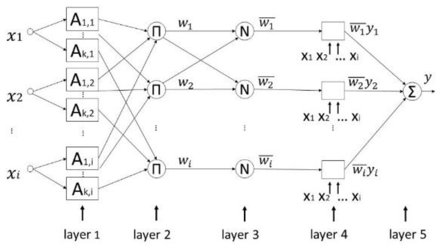
2.2.1. Adaptive Neuro-Fuzzy Inference System (ANFIS)

The adaptive neuro-fuzzy inference system (ANFIS) uses an architecture that is based on both ANN and fuzzy logic principles and takes advantage of the benefits of both in a single framework. It can be described by the fuzzy “IF-THEN” rules from the Takagi and Sugeno (TS) type [106] as follows:
R i : i f   x 1 = A i , 1   a n d a n d   x k = A i , k t h e n   y i = b i , 0 + b i , 1 x 1 + b i , 2 x 2 + + b i , k x k
where A i , k is the membership function associated with input variables x k and n is the number of inputs.
A typical ANFIS network is a five-layer structure consisting of the fuzzy layer, the product layer, the normalized layer, the de-fuzzy layer and the total output layer [3,107,108], as depicted in Figure 1.
In the first layer, every node i represents a linguistic label and is described by the following membership function, as given in Equation (3).
A i , k ( x r ) = e ( ( x r v i , k ) σ ι , κ ) 2 , f o r   r = 1 ,   2 , , i
where A i , k is the membership function which is considered to be Gaussian and is described by the center ν and the spread σ.
In the second layer, the firing strength of the rule is computed using multiplicative operator, as presented in Equation (4). Firing strength is the weight degree of the IF-THEN rule and determines the shape of the output function for that rule.
w i = k = 1 n A i , k ( x k )
In the third layer, the i-th node calculates the ratio of the i-th rule’s firing strength to the sum of the firing strength of all rules. This is the normalization layer which normalizes the strength of all rules and the output of each node is given by Equation (5).
w ¯ i = w i i = 1 w i
In the fourth layer, each node is an adaptive node with a function given by Equation (6). In this layer, each node calculates a linear function where its coefficients are adapted by using the error function of the multilayer feed-forward neural network.
y ¯ i = w ¯ i y i
In the fifth layer, there is only a fixed node indicated as the sum of the net outputs of the nodes in Layer 4. It computes the overall output as the sum of all incoming inputs and is expressed by Equation (7).
y = i y ¯ i
ANFIS uses a hybrid learning algorithm to train the model. The back-propagation algorithm is used to train the parameters in Layer 1, whereas a variation of least-squares approximation or back-propagation algorithm is used for training the parameters of the fourth layer [108,109].

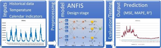
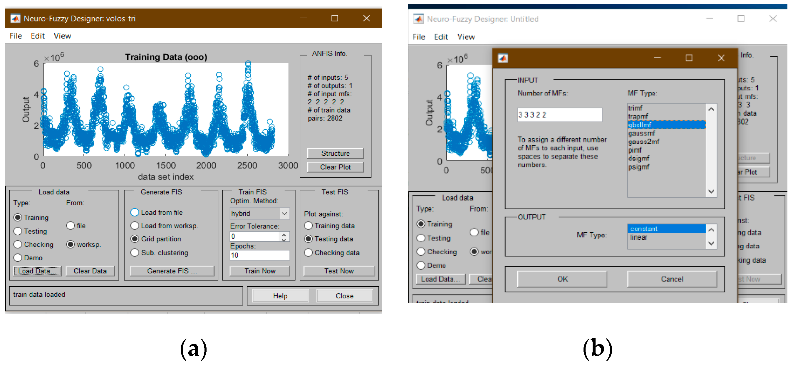
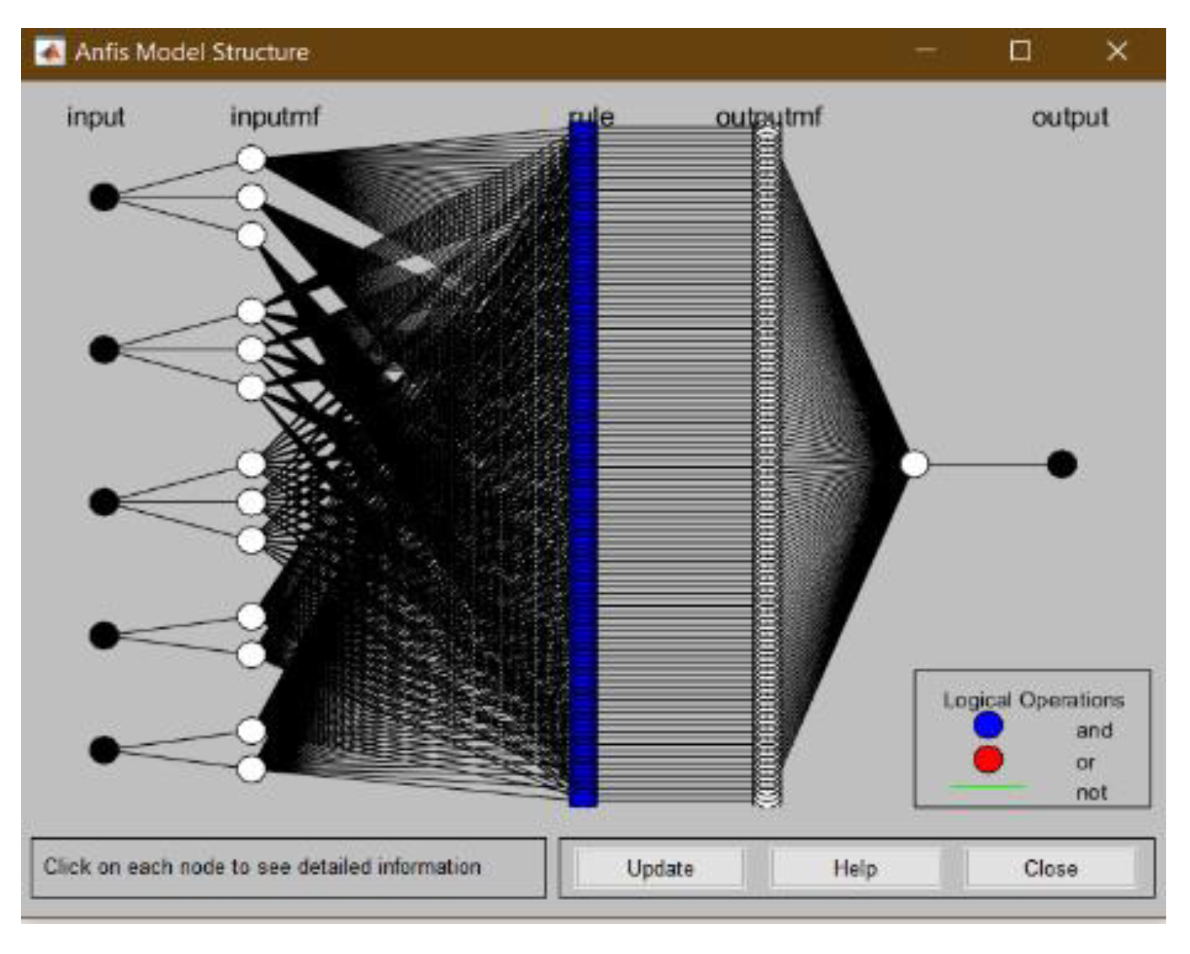
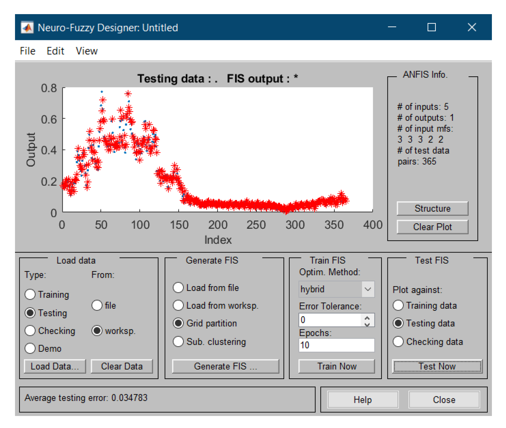
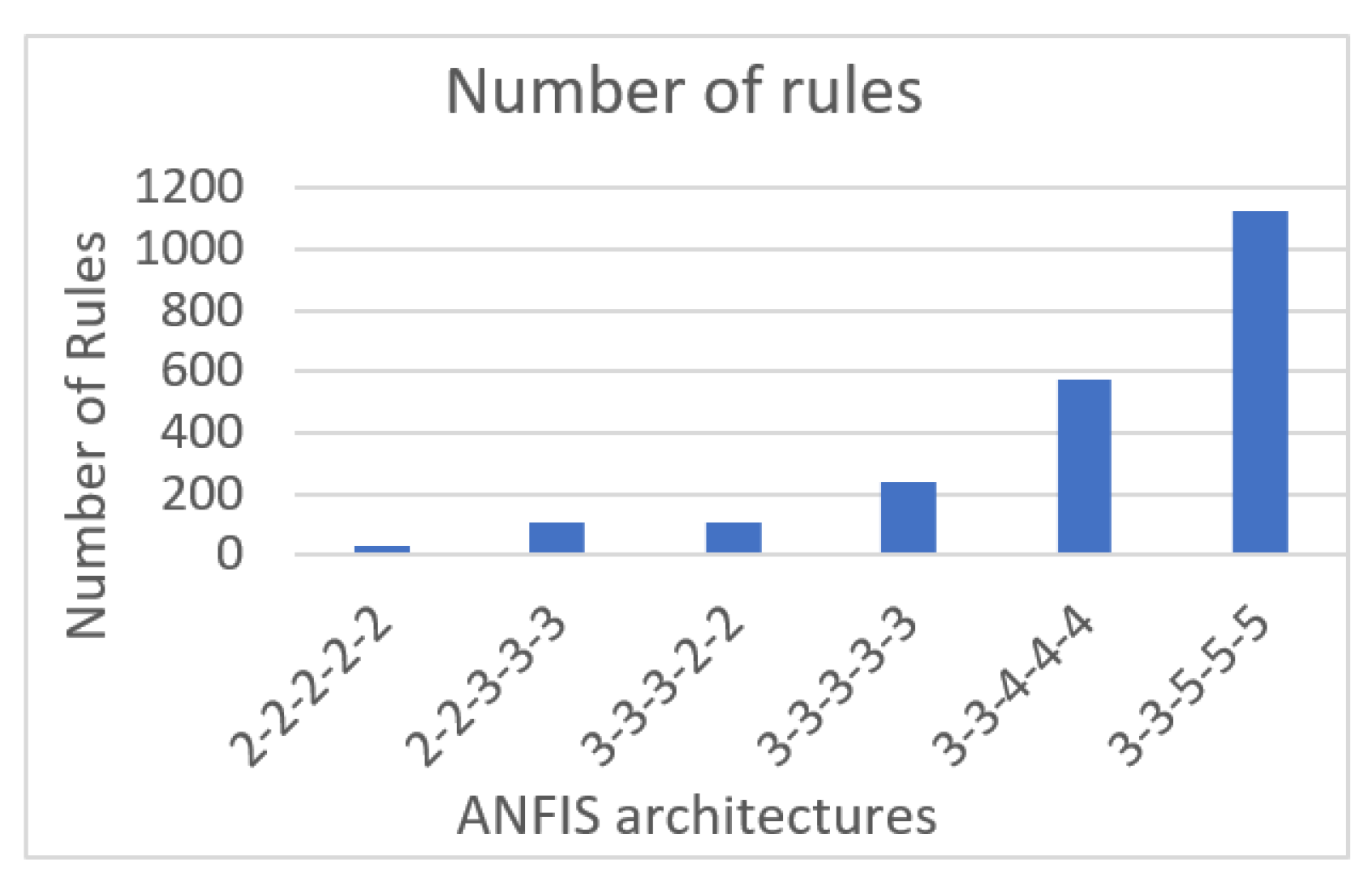
2.2.2. Proposed ANFIS Architecture Applied in Natural Gas Consumption Forecasting

In order to develop an efficient ANFIS model for NG demand forecasting, the authors needed to follow a certain process regarding the design of model’s architecture as well as an exploration process that will properly configure the input and training parameters of the examined model. Priority was given to the definition of the FIS architecture before the training of the network [110]. Among various fuzzy inference system (FIS) models, the Sugeno fuzzy model is the most widely used because of its higher interpretability and computational ability, that includes embedded optimal and adaptive techniques [111]. In order to create a fuzzy rule, the input space needs first to be divided. Two methods are used to divide space, comprised by input variables: the grid partitioning method and the subtractive clustering method. The main difference between these two functions refers to the way the partition of the input space is created.
In grid partitioning [109], the input space is divided into a grid-like structure without overlapping parts. Grid partitioning performs partitioning of the input space using all possible combinations of membership functions of each variable. This method is used when the number of input variables is small. For example, for 10 input variables and two membership functions for each input variable, then the input space is divided into 210 = 1024 specific areas, representing one rule for each specific area, and the total number of rules is 1024, which is a very complicated structure. Therefore, the grid partitioning method is mainly used when the number of input variables is small.
On the other hand, the subtractive clustering method divides the input space into appropriate clusters, even if the user does not specify their number. If the size of the cluster becomes small, then the number of clusters increases, thus increasing the number of fuzzy rules. A rule is created for each cluster, whereas different values for parameters, like range of influence, squash factor, accept ratio and reject ratio, need to be explored for determining an efficient architecture, which will keep the balance between the total number of ANFIS parameters and the total number of rules.
Considering the above specifications, the authors used the Grid partition option to define the FIS architecture due to its simplicity, less time-consuming performance as well as it can easily explore the number and type of membership function (MF). In this stage, the number and type of membership functions of each input variable, along with the rules and values of parameters that belong to these functions, were determined using the option of Grid partition.
When implementing an ANFIS architecture, researchers should have in mind that there is one main restriction: the number of input variables. When these are more than five, then the number of the IF-THEN rules and the computational time also increase, hindering ANFIS to model output with respect to inputs [110]. Thus, in this study, five variables were chosen as input parameters, i.e., month, day, temperature, demand of a day before and demand of current day. As described above, a day-ahead consumption demand was selected as the output variable whose value can be produced by choosing between the option of linear or constant type of MF.
Finding the most efficient ANFIS architecture is a demanding task and entails a rigorous exploration process. Since our concern focuses on the increment of network’s accuracy and decrement of the errors, five necessary configurations should be considered in this direction: (i) the number of membership functions, (ii) types of MF (triangular, trapezoidal, bell-shaped, Gaussian and sigmoid), (iii) types of output MF (constant or linear), (iv) optimization methods (hybrid or back propagation) and (v) the number of epochs [112]. For the convenience of readers, these steps are visually represented in the flowchart in Figure 2.
The aforementioned set of configurations needs to be deployed in order to generate FIS and next to train the ANFIS model. Accordingly, the dataset that included the five input variables (i.e., month, day, temperature, demand of a day before, demand of current day) was selected to determine the only output (day-ahead demand). Initially, the training dataset was loaded in the ANFIS tool, as shown in Figure 3a. The next step was the design of the neuro-fuzzy model using the option “Generate FIS”. The Grid partition option was selected according to the description above (see Figure 3a). These two settings, concerning the fuzzy input variables along with their membership functions, are the most important parts to design the ANFIS. An example of selecting the number and type of MFs is illustrated in Figure 3b.
The number and type of membership function were assigned to the input parameters following the trial-and-error approach. The different types of MF that are offered by the MATLAB ANFIS editor include the triangular, trapezoidal, generalized bell (Gbell), Gaussian curve, Gaussian combination, difference between two sigmoid functions and product of two sigmoid functions (see Figure 3b). Regarding the type of output MFs, in the Sugeno-type fuzzy system, there are two options: a constant-type conclusion or a linear-type conclusion function. In the case of linear function, the output y is defined as:
y = k 0 + k 1 x 1 + k 2 x 2 + + k n x n
where x1, x2, , xn are the n inputs. In this case, ANFIS needs to define k0, k1, k2 up to kn, and it is very time consuming to efficiently calculate the outputs when a large number of parameters are considered. On the other hand, when a constant MF is selected, the algorithm needs to define only one parameter to provide a reliable forecasted value. Thus, the computational time is really low.
The selected configuration also includes the hybrid optimization method, while the number of epochs selected to train the model was between 10 and 50. The hybrid optimization method uses the back propagation learning algorithm for parameters associated with input MF and the least-square estimation algorithm for parameters associated with output MF; thus, it was selected as the most proper one [113]. Various sets of ANFIS configurations are presented in Table 3, regarding different sets of number for MFs, as considered by the authors of this work.
Regarding the output MFs, constant and linear MF were accordingly investigated after certain numbers of experiments conducted. From these experiments and for the linear output, it was observed that the number of rules increases significantly, as well as the computational time, even in the case of problems with a small number of inputs (see Table A1 in Appendix A). Thus, the linear type was not considered as an appropriate parameter of output MF since it is extremely time consuming. In this context, the trial-and-error approach was followed for the selection of the input-output type of MFs. Figure 4 illustrates an indicative ANFIS model, which was constructed with the following configuration set: 3-3-3-2-2, gbell MF, constant output MF, 10 epochs, hybrid.

2.2.3. Testing and Evaluation

The testing process for the ANFIS model was accomplished by using the testing data, which were completely unknown to the model. The predictor makes predictions on each day and finally compares the calculated predicted value with the real value. For example, considering the city of Volos, the predicted values that are illustrated in red in Figure 5 are compared with the real values (in blue color).
In order to evaluate the prediction of NG demand, five well known and commonly used statistical indicators were introduced, i.e., mean square error (MSE), root mean square error (RMSE), mean absolute error (MAE), mean absolute percentage error (MAPE) and coefficient of determination (R2). The mathematical equations of the statistical indicators are described below.
  • Mean squared error:
    MSE = 1 T t = 1 T ( Z ( t ) X ( t ) ) 2
  • Root mean squared error:
    R MSE = MSE
  • Mean absolute error:
    MAE = 1 T t = 1 T | Z ( t ) X ( t ) |
  • Mean absolute percentage error:
    MAPE = 1 T t = 1 T | Z ( t ) X ( t ) Z ( t ) |
  • Coefficient of determination:
    R = T t = 1 T Z ( t ) · X ( t ) ( t = 1 T Z ( t ) ) ( t = 1 T X ( t ) ) T t = 1 T ( Z ( t ) ) 2 ( t = 1 T Z ( t ) ) 2 · T t = 1 T ( X ( t ) ) 2 ( t = 1 T X ( t ) ) 2
    where X(t) is the forecasted value of the NG at the t-th iteration, and Z(t) is the actual value of the NG at the t-th iteration, t = 1, , T, where T is the number of testing records.
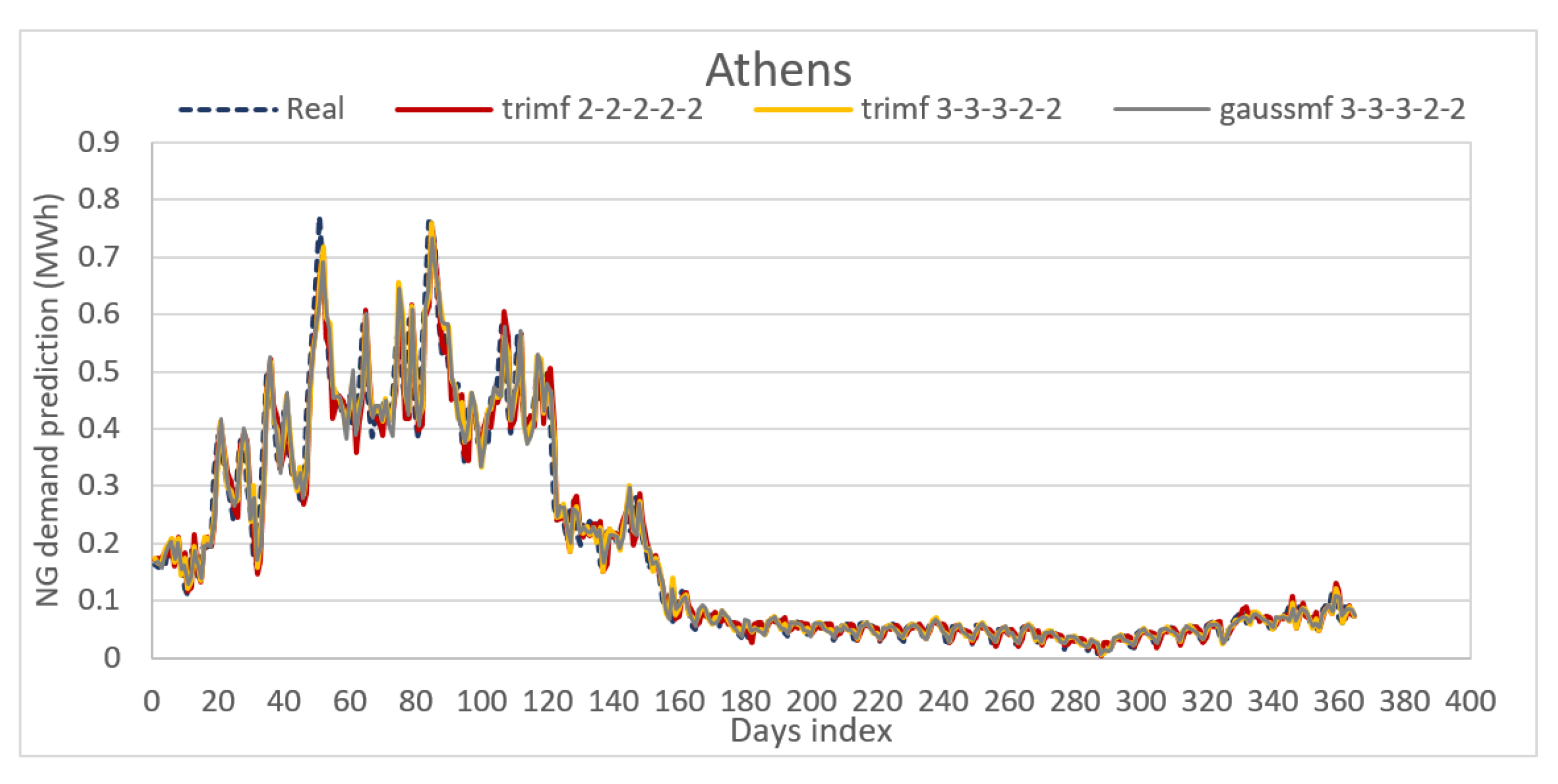
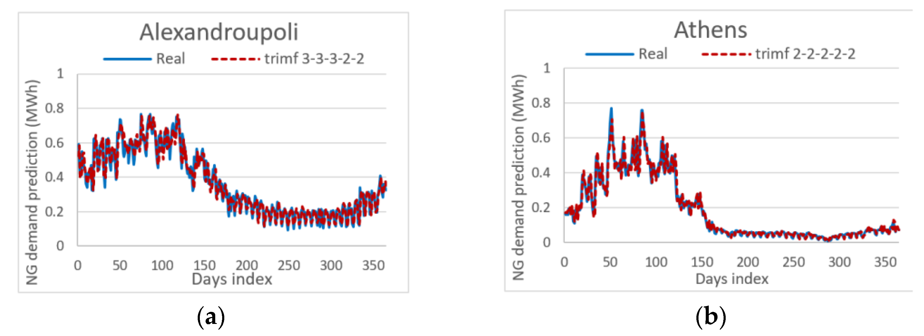
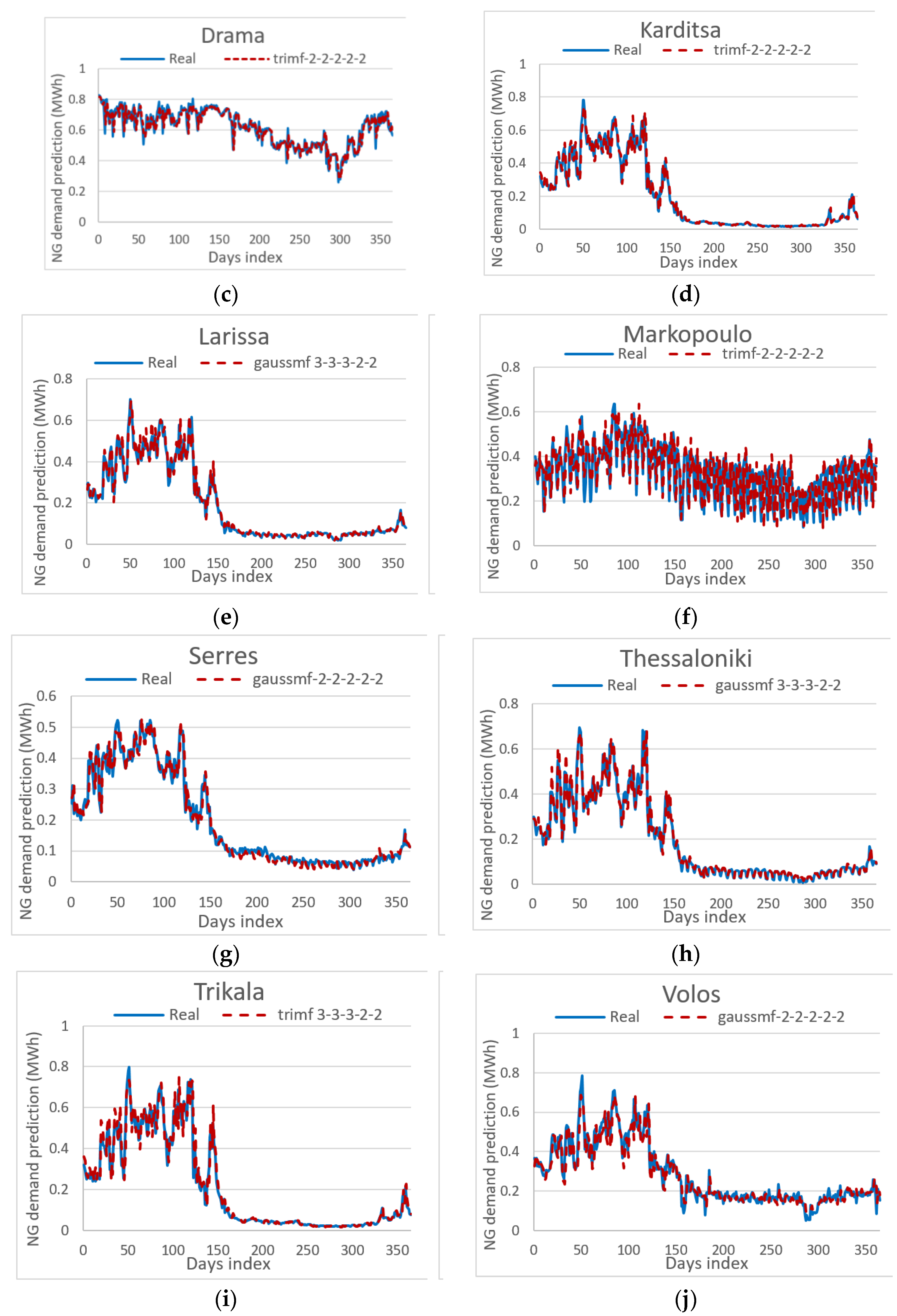
Higher values of R2, i.e., closer to 1, mean better model performance and the regression line fits the data well. A coefficient of determination value of 1.0 points out that the regression curve fits the data perfectly.

3. Results

This section presents the exploration analysis results for the various ANFIS architectures as proposed in Section 2.2.2. Considering the steps proposed in Section 2.2, the initial dataset is split into training and testing. During the training process, the ANFIS model is designed for each one of the suggested configurations. After the training process of the ANFIS finishes, NG consumption demands for the next day (one day ahead prediction) are calculated from the generated FIS. The NG consumption results only for the city of Athens (as an indicative example) regarding all configurations tested, are presented in Table 4, whereas Table 5 gathers the best three results of NG consumption demand obtained from ANFIS for each of the 10 cities. To evaluate the performance of the models, the statistical indicator mean absolute percent error (MAPE) was used [91]. MAPE is a relative measurement, independent of scale, and it is the most common performance metric in time series forecasting, due to being reliable and valid [21].
The corresponding graphical representation of the results regarding the best three out of 47 total ANFIS architectures for the city of Athens is illustrated in Figure 6. Also, the best ANFIS model for each city can be found in Table 6, which provides the most reliable ANFIS architecture results for each city. All the results have been previously ranked, based on the minimum value of MAPE and subsequently the minimum values of MSE, RMSE and MAE. The priority was given to MAPE as one of the most crucial evaluation metrics, according to the literature [91,96], which was used in this study to compare various models obtained from ANFIS and other soft computing and neural networks methods. As a relative and easy to interpret measurement, MAPE is reliable, valid and independent of scale. The smaller the values of MAPE are, the closer the forecasted values are to the actual values.
As illustrated in Table 6, ANFIS models appear to perform best mostly when triangular MFs are used for the input variables: three MFs for the first three input variables (month, day of week and mean temperature) and two or three MFs for the other two input variables (daily demand for current day and one day before). Also, constant MFs are selected for the output variable and hybrid optimization method. The graphical representation of the best ANFIS models for each city is illustrated in Figure 7.
It is worth mentioning that all three most efficient ANFIS architectures with respect to MAPE values have triangular or gaussian MFs and 2-2-2-2-2 or 3-3-3-2-2 number of input MFs, whereas the output MF is constant and the learning algorithm is hybrid. In addition, the application of other MFs combinations does not seem to give results that could be on top of the list. Due to the limitation of the total number of parameters that should not exceed the number of training data pairs, the number of MFs was chosen based on the number of input parameters. Figure 8 shows the exponential increase in the number of rules when the number of MFs increases, whereas Table A2 in Appendix A gathers the time and number of rules for all the proposed ANFIS configurations.

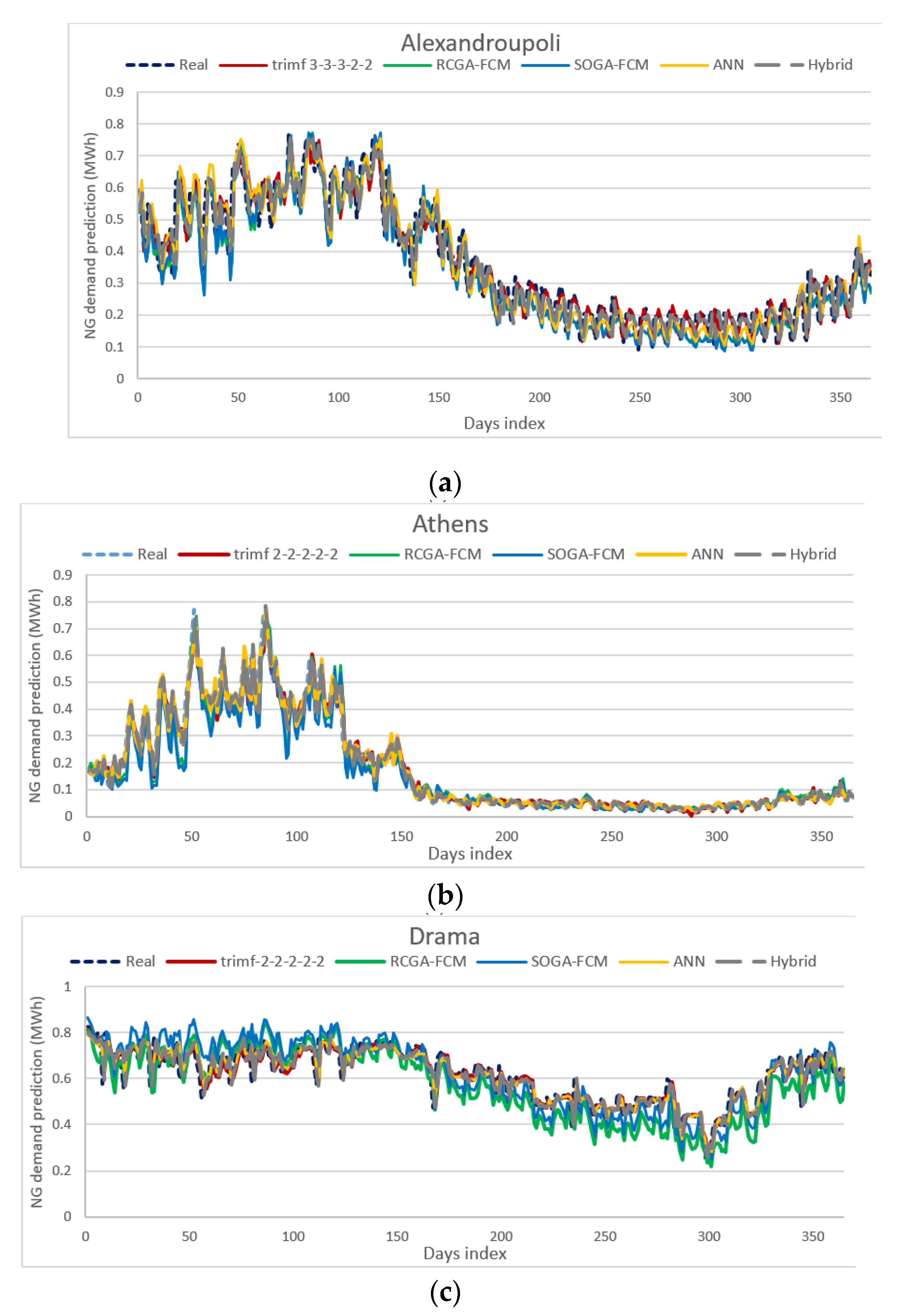
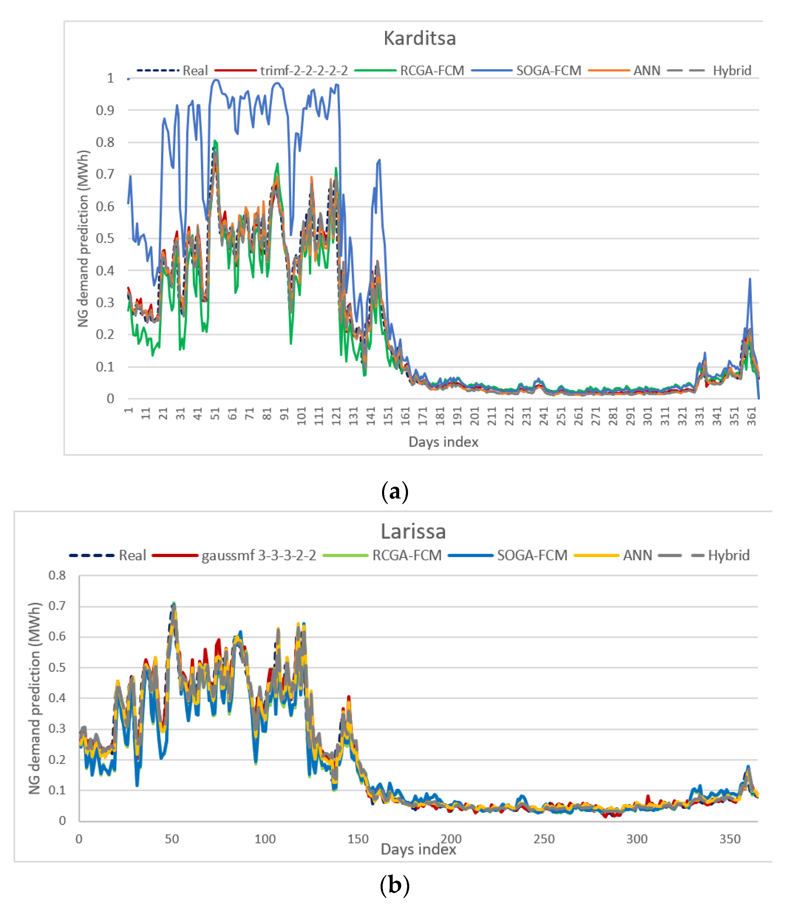
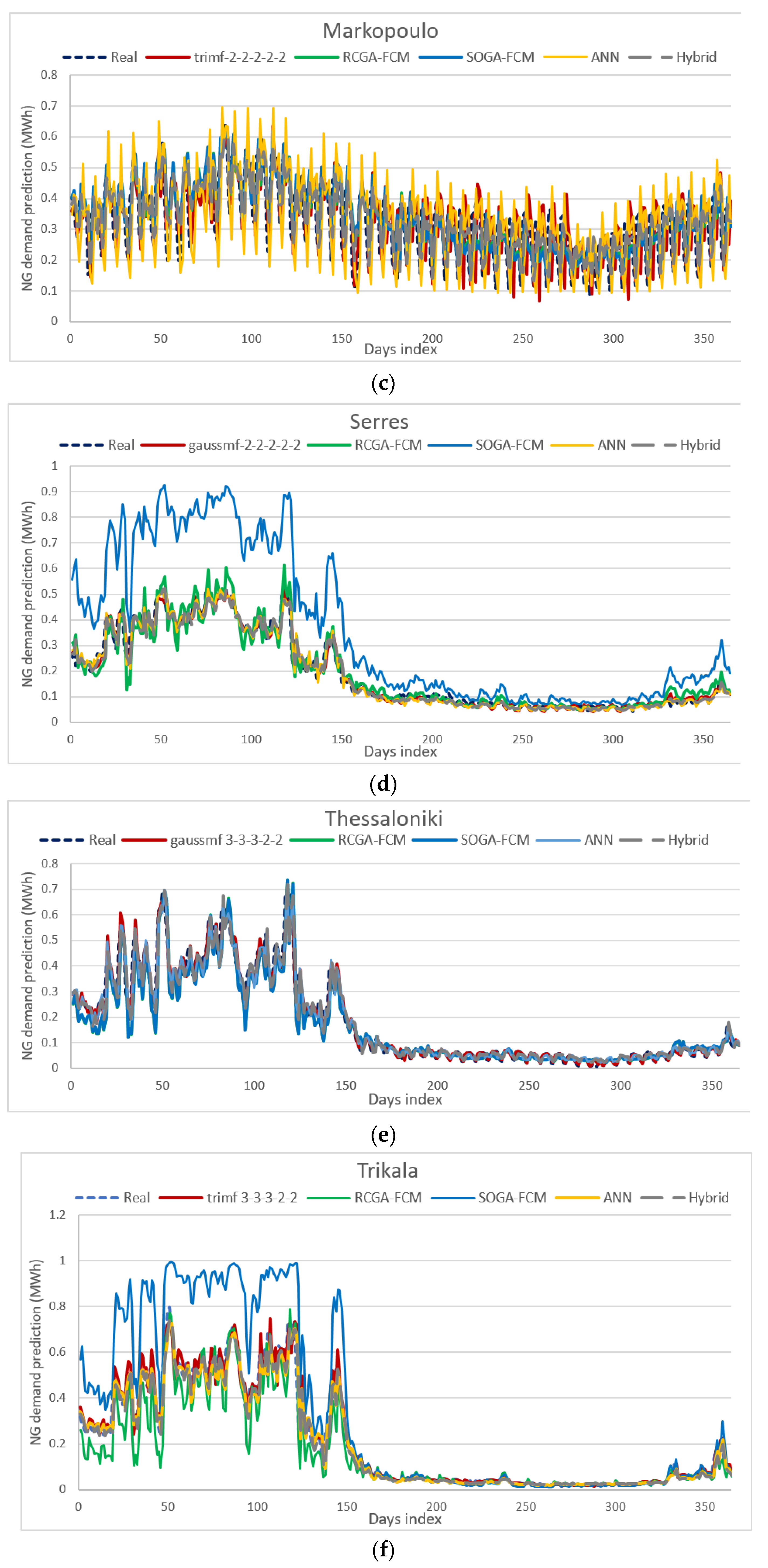
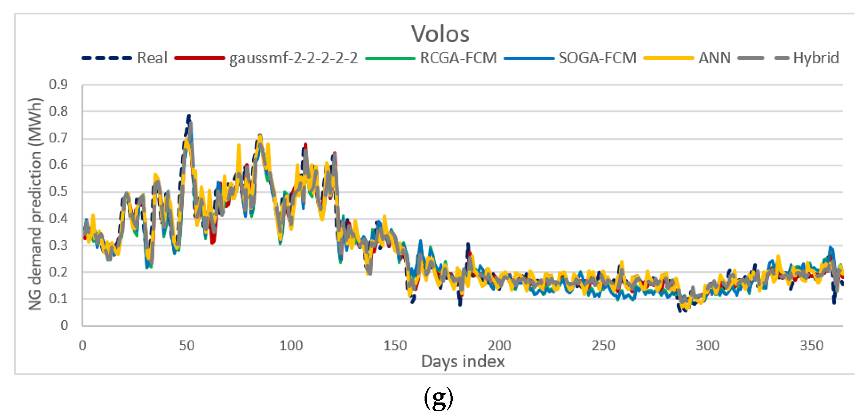
3.1. Comparison with ANNs, FCMs and Hybrid FCM-ANN

To further investigate the performance of the proposed ANFIS architectures, an extensive comparative analysis between the state of the art ANNs, soft computing methods of FCMs and their hybrid combination of FCMs with ANNs was performed.
The architecture of the analyzed ANN was a multilayer feed forward network with an input layer containing five inputs (month, day, temperature, demand of a day before, current demand), a hidden layer with 10 neurons, and an output layer with one output (a day-ahead demand prediction). The authors used the sigmoidal activation function in all layers and implemented Levenberg–Marquardt algorithm to train the network.
The soft computing method of fuzzy cognitive map with evolutionary learning capabilities, such as the real-coded genetic algorithm (RCGA-FCM) and structure optimization genetic algorithm (SOGA-FCM) [100], were used for time series modeling and prediction of day-ahead NG energy demand. For FCM learning, we implemented RCGA-FCM and SOGA-FCM. A short description on the applied evolutionary-based FCM approaches is given in Appendix B. The implementations of FCMs differ from ANFIS, even though they both belong to the soft computing family.
In this research study, we used the dynamic model type (Equation (B1)) which is found in Appendix B, with sigmoidal transformation function. FCMs learned with the use of RCGA and SOGA algorithm contain five concepts (month, day, temperature, demand of a day before, current demand) [114].
The applied hybrid approach for time series prediction is based on FCMs and ANNs and was previously proposed in [18,19]. It allows us to select the most significant concepts for FCM using SOGA. These concepts are used as the inputs for ANN. In the hybrid approach, we used artificial neural networks with an input layer with five inputs selected by the SOGA-FCM approach, a hidden layer with 10 neurons and an output layer with one output (one day-ahead demand prediction). Sigmoidal activation function and Levenberg–Marquardt learning algorithm were used. All the simulations for FCMs and hybrid FCM-ANN configurations were performed with the software tool ISEMK [115] which has been developed for time series forecasting purposes. An analytical description of FCM-based models and hybrid FCM-ANN can be found in [13,101,102,116], whereas they are used in this work only for comparison purposes.
In what follows, Table 7 gathers the results of the explored ANN and soft computing models, which are straightforward compared with our best performed ANFIS configuration, for each one out of the 10 cities, suggested in this research work. In Figure 9, three indicative graphs of the cities Alexandroupoli, Athens, and Drama are illustrated regarding the predicted values of NG demand for all the best proposed architectures. In Appendix A, the corresponding graphs of the rest of the cities are presented (see Figure A1).
For a deeper analysis of the examined architectures (ANFIS, ANN, FCM, hybrid FCM-ANN), the authors report on further details regarding the parameters of each model used in this study. The ANN and FCM models were previously applied for NG demand prediction in several research works, such as those in [13,101,102,116]. The models were sufficiently described and the hyperparameters were properly configured to offer optimum performance of the investigated FCM models.
Table 8 depicts the optimum parameters for all cities considering the neural and FCM evolutionary methods (ANN, RCGA-FCM, SOGA-FCM, Hybrid), compared with the proposed best performed ANFIS. The average running time is also presented in Table 8, which was calculated for each soft computing architecture for all models. It is worth mentioning that we have conducted a rigorous exploratory analysis for all the investigated neuro-fuzzy, soft computing techniques and ANNs, with different parameters, for training and model optimization, to reach the highest prediction accuracy with respect to the evaluation metrics.

3.2. Discussion of Results

In this work, several ANFIS architectures were investigated, with respect to all the variables that were carefully determined in the developed model as reported in Section 2.1 and after different sets of model configurations were tested. However, only one ANFIS architecture reached the optimum performance, in terms of forecasting accuracy, considering the minimum value of MAPE and subsequently the minimum values of MSE, RMSE and MAE values produced. In particular, it emerged that the optimum ANFIS configuration is 2-2-2-2-2 with triangular MFs for input variables, which produces the most simple (concerning the number of rules), fast (see Table A2 in Appendix A) and accurate model for this energy forecasting problem. In general, it is observed that the best results are produced from the combination of triangular or gaussian MFs regarding the input variables, and the constant MFs regarding the output layers.
To further discuss the results produced and to show the effectiveness of the proposed forecasting methodology of ANFIS, the authors conducted a comparative analysis regarding the forecasting performance between the proposed technique, and other ANN and soft computing methods too, such as FCM, which were reported in the literature and have already been applied in the specific domain. The MAPE criterion was used to compare various models from ANN, evolutionary FCM, Hybrid FCM-ANN and ANFIS. The results are given in Table 7. For example, the MAPE values of RCGA-FCM, SOGA-FCM, ANN, hybrid and ANFIS models for the city of Alexandroupoli were calculated as 17.62%, 17.17%, 16.11%, 14.30% and 10.11%, respectively. The smaller the values of MAPE are, the closer to the actual values the forecasted values are. The best result was obtained from the ANFIS model. The respective figures in the text and in Appendix A have been updated with the new prediction values.
Considering the same dataset linked to only three cities (Athens, Thessaloniki, and Larissa) out of the ten that participated in our study, a day-ahead NG consumption prediction was investigated in [117], applying ANN and LSTM approaches and in [102], implementing the SOGA-FCM method and a hybrid combination of it. Furthermore, an ensemble FCM prediction methodology concerning the same dataset was presented in [13], in which a recent soft computing technique for time series forecasting, using evolutionary fuzzy cognitive maps and their ensemble combination was compared to ANNs, as benchmark forecasting methods. These methods and their results in terms of MSE and MAE values for three benchmark cities are all gathered in the following table and certain results can be concluded. The main reason for selecting the statistical indicators MSE and MAE in the following figure is to accomplish a straightforward comparison with the results published in previous works.
In Figure 10, it can be noted that all methods achieve high accuracy in NG consumption predictions, using the same dataset. The best ANFIS approach seems to excel over the ensemble and hybrid methods. Consequently, the proposed ANFIS architecture, which handles the fuzziness of data more efficiently, outperforms all the other examined methods in most cases, with a rather remarkable difference. ANFIS is less time consuming and more flexible than ANN, and as it employs fuzzy rules and membership functions incorporating with real-world systems, it can be used as alternate method to ANN forecasting.
It is observed that the proposed method exhibits better or similar performance to other well-known ANN, FCM or hybrid FCM-ANN architectures for the ten cities under investigation. The produced results highlight the significance and superiority of neuro-fuzzy methods over the other examined methods in terms of prediction accuracy, when they deal with time series forecasting problems in energy. This is in accordance with the main advantageous features of ANFIS models, which are their ability to capture the nonlinear structure of a process, their adaptation capability, and fast training characteristics. As reported in the literature, ANFIS models are able to cope with the uncertainty and fuzziness that characterize the energy domain [118,119] when other intelligent methods cannot tackle them.
The main outcomes of this study can be summarized as follows:
  • The proposed ANFIS method exhibits the best performance when certain configuration settings are selected for the examined datasets which are linked to ten cities of Greece. The authors concluded that a certain configuration is best for the examined ANFIS model, after having conducted a number of experiments and following a trial-and error approach. The best ANFIS model is based on a distinct architecture that features a 2-2-2-2-2 triangular or gaussian MF.
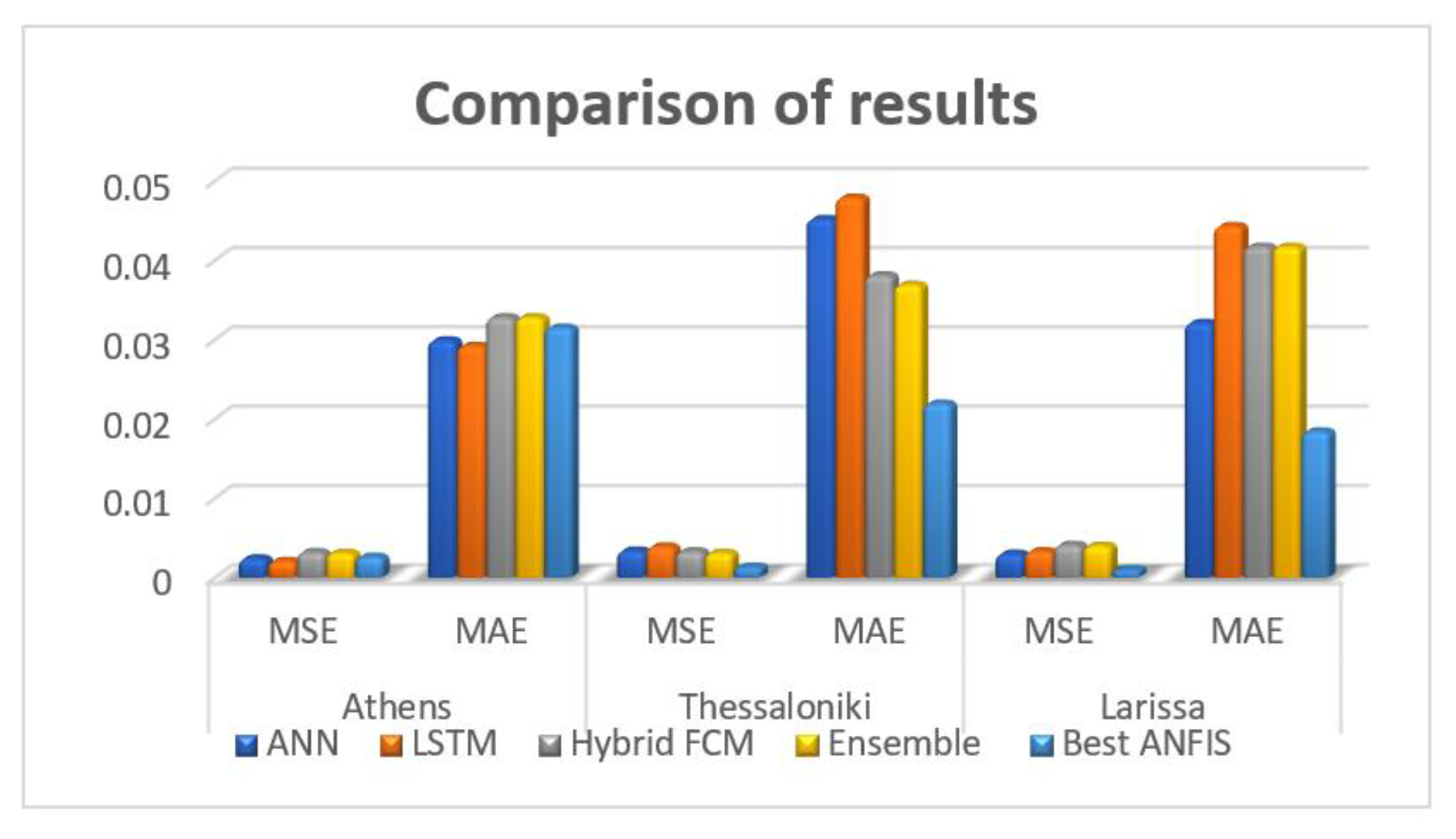
  • The proposed ANFIS architecture is superior to the four benchmark and well-known ANN and FCM methods (ANN, SOGA-FCM, RCGA-FCM, Hybrid FCM-ANN), which have been efficiently used in NG consumption forecasting. The results presented in Table 7, which gathers various error indicators and the R2, as prediction accuracy indices for all five architectures, show that the best ANFIS model holds the best prediction accuracy among all the methods that were included in this comparative analysis.
  • The proposed ANFIS model shows significant capacity when applied to forecasting NG demand, since it exhibits better performance (see Table 7) with less running time (see Table 8) and more flexibility to handle fuzziness than other well-known ANN and FCM architectures.

4. Conclusions

This study proposes the ANFIS method to predict short-term demand of NG consumption. This approach is applied on the Greek territory and uses 10 different datasets provided by DESFA, that regard previous energy consumption historical data, for ten main cities. To decide the model’s proper architecture, the authors follow an exploration process regarding the best configuration of input and training parameters. The best ANFIS model is then compared to other well-known ANN and soft computing models that are commonly used for energy demand prediction purposes. The ANFIS method demonstrates significant performance in the field of energy demand prediction, outweighing the traditional ANN and FCM architectures. In addition, the running time of the proposed architecture is much less than those of other examined models, making it the right decision for day-ahead demand forecasting of NG. The findings of this study reveal that the highest forecasting accuracy emerged when the same model configuration was used for most of the cities, highlighting the generalization capabilities of the proposed architecture.
This work can be widely used in short-term demand forecasting for other countries too, with the same or similar input parameters, and can be also useful especially for distribution operators, providing them with the ability to make long-term planning decisions and apply the correct strategic policies in this direction. Following the literature, the ANFIS approach can be applied in various other domains such as medicine, environmental modelling, various energy systems, like solar and wind, as well as other engineering applications. As can be seen, the ANFIS application area is wide, and as regards the energy sector, this method finds great applicability due to its high prediction accuracy, robustness, and easiness to use.
The results show that the proposed algorithm, which was proven to be efficient, fast and robust, can be adopted by regulatory authorities and decision makers to perform rigorous forecasting of natural gas demand for the respective case cities and other cities in Greece too. The investigated approach is an accurate estimation method as it makes efficient short-term predictions in natural gas demand, showing minor deviations between the real and the predicting values. Since short-term natural gas forecasting is mostly used for the timely reservation of transport, storage capacity optimization, timely purchase of natural gas deliveries and capacity allocation, this method becomes critical to determine the energy policy for Greece and the wider area too, having overall a positive impact in natural gas consumption.
Future work is oriented in developing more advanced neuro-fuzzy models providing explainability and transparency in prediction tasks in diverse research domains, in order to evaluate the generalization capabilities of this approach. Furthermore, new forecast combination architectures of efficient deep learning and regularized recurrent neural networks for time series modelling and prediction in the energy sector will be investigated.

Author Contributions

Conceptualization, E.I.P. and E.I.P.; methodology, E.I.P.; software, E.I.P., K.P. (Konstantinos Papageorgiou) and K.P. (Katarzyna Poczeta); validation, E.I.P., E.I.P., K.P. (Konstantinos Papageorgiou), K.P. (Katarzyna Poczeta), D.B. and G.S.; formal analysis, E.I.P. and E.I.P.; investigation, E.I.P.; resources, E.I.P.; data curation, E.I.P. and K.P. (Konstantinos Papageorgiou), K.P. (Katarzyna Poczeta); writing—original draft preparation, E.I.P.; writing—review and editing, K.P. (Katarzyna Poczeta), E.I.P., D.B. and G.S.; visualization, E.I.P.; supervision, E.I.P. and G.S.; project administration, E.I.P. and D.B. All authors have read and agreed to the published version of the manuscript.

Funding

This research received no external funding.

Conflicts of Interest

The authors declare no conflict of interest.

Appendix A

Table A1. Different configurations of the selected ANFIS architectures regarding linear output MF.
Type of Input MFNumber of MFsType of Output MFNumber of RulesMSERMSEMAEMAPER2Time (s)
trimf2-2-2-2-2Linear320.0011950.0345720.01942611.721800.982121148
trapmf2-2-2-2-2Linear320.0013580.0368590.02086112.123780.979559148
gbellmf2-2-2-2-2Linear320.0012670.0356030.01992111.464460.980963148
Gaussmf2-2-2-2-2Linear320.0012980.0360380.02025911.977940.980468148
Gauss2mf2-2-2-2-2Linear320.0014060.0374960.02087811.263820.978860148
pimf2-2-2-2-2Linear320.0016350.0404420.02217612.082980.975405148
dsigmf2-2-2-2-2Linear320.0014230.0377330.02106211.267210.978592148
psigmf2-2-2-2-2Linear320.0014230.0377330.02106211.267220.978592148
trimf2-2-3-3-3Linear1080.0014760.0384300.02094111.178620.977773328
Gaussmf2-2-3-3-3Linear1080.0020380.0451490.02328612.717200.969241328
Table A2. Running time and number of rules for all the proposed ANFIS configurations.
Type of Input MFNumber of MFsType of Output MFNumber of EpochsOptimizationNumber of RulesTime Run
trimf, trapmf, gbell, gauss, pim, sigm2-2-2-2-2Constant10Hybrid327 s
trimf, trapmf, gbell, gauss, pim, sigm2-2-3-3-3Constant10Hybrid10811 s
trimf, trapmf, gbell, gauss, pim, sigm3-3-3-2-2Constant10Hybrid10819 s
trimf, trapmf, gbell3-3-3-3-3Constant10Hybrid24368 s
trimf3-3-4-4-4Constant10Hybrid57610 min 10 s
trimf3-3-5-5-5Constant10Hybrid112540 min
trapmf3-3-4-4-4Constant10Hybrid57612min
trapmf3-3-5-5-5Constant10Hybrid112570 min
gbellmf3-3-4-4-4Constant10Hybrid57612 min 35 s
gbellmf3-3-5-5-5Constant10Hybrid112550 min
gaussmf3-3-3-3-3Constant10Hybrid2434 min
gaussmf3-3-4-4-4Constant10Hybrid57625 min
gaussmf3-3-5-5-5Constant10Hybrid112547 min
gauss2mf3-3-3-3-3Constant10Hybrid2434 min
gauss2mf3-3-4-4-4Constant10Hybrid57625 min
gauss2mf3-3-5-5-5Constant10Hybrid112547 min
pimf3-3-3-3-3Constant10Hybrid2433.5 min
pimf3-3-4-4-4Constant10hybrid57620 min
pimf3-3-5-5-5Constant10hybrid112542 min
Figure A1. Comparison of forecasting results for each city considering all examined methods. (a) Testing for Karditsa, (b) testing for Larissa, (c) testing for Markopoulo, (d) testing for Serres, (e) testing for Thessaloniki, (f) testing for Trikala, (g) testing for Volos.
Energies 13 02317 g0a1aEnergies 13 02317 g0a1bEnergies 13 02317 g0a1c

Appendix B

Appendix B.1. Fuzzy Cognitive Maps

Fuzzy cognitive maps (FCMs) are an effective tool for modeling and predicting time series. The structure of the FCM model is based on a directed graph, the nodes of which denote concepts significant for the analyzed problem, and the links are the causal relationships. Values of concepts can change over time according to the adopted dynamics model, for example the nonlinear dynamics model:
X i ( t + 1 ) = F ( X i ( t ) + j = 1 j i n X j ( t ) · w j , i )
where Xi(t) is the value of the i-th concept at the t-th iteration, wj,i is the weight of the causal relationship between concepts Xj and Xi taking values from the range [−1,1], t is discrete time, i,j = 1, 2, …, n, n is the number of concepts, and F is the transformation function normalizing the factor values to the range [0,1] or [−1,1]. Fuzzy cognitive maps can be constructed based on expert knowledge or with the use of machine learning algorithms. The aim of fuzzy cognitive map learning is to determine the weights of the causal relationships between concepts on the basis of available time series.
An effective method for fuzzy cognitive map learning is the real-coded genetic algorithm (RCGA) [100]. RCGA defines each individual in the population based on a floating-point vector containing the causal relationships. Each individual is decoded into a candidate map and evaluated with the use of proper fitness function. We used the following fitness function:
f i t n e s s p ( e r o r r l ) = 1 a · e r o r r l + 1
where a is a parameter, l is the number of generations, l = 1, …, L, L is the maximum number of generations, p is the number of individuals, p = 1, , P, P is the population size, and e r o r r l is the learning error that can be in the following form:
e r o r r l = 1 T t = 1 T ( Z ( t ) X ( t ) ) 2
where X(t) is the predicted value of the decision concept at the t-th iteration, Z(t) is the real normalized value of the decision concept at the t-th iteration, t = 1, , T, and T is the number of learning records.
Another way of learning fuzzy cognitive maps is the structure optimization genetic algorithm (SOGA) [100,120]. This allows one to simplify the structure of the FCM model by selecting the most significant concepts and causal relationships during the learning process. In this approach, the fitness function is based on the modified learning error including an additional penalty for highly complexity of the candidate fuzzy cognitive map, understood as a large number of concepts and non-zero relationships, described as follows:
e r o r r l = e r o r r l + b 1 n r n 2 e r o r r l + b 2 n c n e r o r r l
where b1, b2 are the learning parameters, nc is the number of the concepts in the candidate FCM model, nr is the number of the non-zero relationships between concepts, n is the number of all possible concepts, and e r o r r l is the learning error type (Equation (A3)).
In this paper, we also used the hybrid approach for time series prediction based on fuzzy cognitive maps with the structure optimization genetic algorithm and artificial neural networks [101]. In the first stage of this approach, the most important concepts are selected with the use of FCMs and the SOGA algorithm. In the second stage, these concepts are used as inputs for the artificial neural network in order to increase the prediction accuracy. The above algorithms have been implemented in the developed ISEMK system [101].

References

  1. Lee, Y.-S.; Tong, L.-I. Forecasting energy consumption using a grey model improved by incorporating genetic programming. Energy Convers. Manag. 2011, 52, 147–152. [Google Scholar] [CrossRef]
  2. Barak, S.; Sadegh, S.S. Forecasting energy consumption using ensemble ARIMA–ANFIS hybrid algorithm. Int. J. Electr. Power Energy Syst. 2016, 82, 92–104. [Google Scholar] [CrossRef] [Green Version]
  3. Adedeji, P.; Akinlabi, S.; Madushele, N.; Olatunji, O. Hybrid Adaptive Neuro-fuzzy Inference System (ANFIS) for a Multi-campus University Energy Consumption Forecast. Int. J. Ambient Energy 2020, 41, 1–20. [Google Scholar] [CrossRef]
  4. Yu, S.; Wei, Y.-M.; Wang, K. A PSO-GA optimal model to estimate primary energy demand of China. Energy Policy 2012, 42, 329–340. [Google Scholar] [CrossRef]
  5. U.S. Energy Information Administraton. International Energy Outlook. 2016. Available online: https://www.eia.gov/outlooks/ieo/pdf/0484(2016)pdf (accessed on 3 January 2020).
  6. Wei, N.; Li, C.; Li, C.; Xie, H.; Du, Z.; Zhang, Q.; Zeng, F. Short-Term Forecasting of Natural Gas Consumption Using Factor Selection Algorithm and Optimized Support Vector Regression. J. Energy Res. Technol. 2018, 141, 032701. [Google Scholar] [CrossRef]
  7. Tamba, J.G.; Ndjakomo, S.; Sapnken, E.; Koffi, F.; Nsouandele, J.L.; Soldo, B.; Njomo, D. Forecasting Natural Gas: A Literature Survey. Int. J. Energy Econ. Policy 2018, 8, 216–249. [Google Scholar]
  8. Salehnia, N.; Falahi, M.A.; Seifi, A.; Adeli, M.H.M. Forecasting natural gas spot prices with nonlinear modeling using Gamma test analysis. J. Nat. Gas Sci. Eng. 2013, 14, 238–249. [Google Scholar] [CrossRef]
  9. Xu, G.; Wang, W. Forecasting China’s natural gas consumption based on a combination model. J. Nat. Gas Chem. 2010, 19, 493–496. [Google Scholar] [CrossRef]
  10. Agbonifo, P.E. Natural Gas Distribution Infrastructure and the Quest for Environmental Sustainability in the Niger Delta: The Prospect of Natural Gas Utilization in Nigeria. Int. J. Energy Econ. Policy 2016, 6, 442–448. [Google Scholar]
  11. Solarin, S.A.; Ozturk, I. The relationship between natural gas consumption and economic growth in OPEC members. Renew. Sustain. Energy Rev. 2016, 58, 1348–1356. [Google Scholar] [CrossRef]
  12. Panapakidis, I.P.; Dagoumas, A.S. Day-ahead natural gas demand forecasting based on the combination of wavelet transform and ANFIS/genetic algorithm/neural network model. Energy 2017, 118, 231–245. [Google Scholar] [CrossRef]
  13. Papageorgiou, K.; Papageorgiou, E.; Poczeta, K.; Gerogiannis, V.; Stamoulis, G. Exploring an Ensemble of Methods that Combines Fuzzy Cognitive Maps and Neural Networks in Solving the Time Series Prediction Problem of Gas Consumption in Greece. Algorithms 2019, 12, 235. [Google Scholar] [CrossRef] [Green Version]
  14. Ediger, V.Ş.; Akar, S. ARIMA forecasting of primary energy demand by fuel in Turkey. Energy Policy 2007, 35, 1701–1708. [Google Scholar] [CrossRef]
  15. Šebalj, D.; Mesaric, J.; Dujak, D. Predicting Natural Gas Consumption—A Literature Review. In Proceedings of the Central European Conference on Information and Intelligent Systems, Varaždin, Croatia, 27–29 September 2017. [Google Scholar]
  16. Gil, S.; Deferrari, J. Generalized Model of Prediction of Natural Gas Consumption. J. Energy Res. Technol. 2004, 126, 90–98. [Google Scholar] [CrossRef]
  17. Akpınar, M.; Yumuşak, N. Estimating household natural gas consumption with multiple regression: Effect of cycle. In Proceedings of the 2013 International Conference on Electronics, Computer and Computation, ICECCO 2013, Ankara, Turkey, 7–9 November 2013; pp. 188–191. [Google Scholar]
  18. Akpinar, M.; Yumusak, N. Day-ahead natural gas forecasting using nonseasonal exponential smoothing methods. In Proceedings of the 2017 IEEE International Conference on Environment and Electrical Engineering and 2017 IEEE Industrial and Commercial Power Systems Europe (EEEIC/I CPS Europe), Milan, Italy, 6–9 June 2017; pp. 1–4. [Google Scholar]
  19. Akpınar, M.; Yumuşak, N. Forecasting household natural gas consumption with ARIMA model: A case study of removing cycle. In Proceedings of the 2013 7th International Conference on Application of Information and Communication Technologies, Baku, Azerbaijan, 23–25 October 2013; pp. 1–6. [Google Scholar]
  20. Deka, A.; Hamta, N.; Esmaeilian, B.; Behdad, S. Predictive Modeling Techniques to Forecast Energy Demand in the United States: A Focus on Economic and Demographic Factors. In Proceedings of the Journal of Energy Resources Technology, Boston, MA, USA, 2–5 August 2015; Volume 138. [Google Scholar]
  21. Kaynar, O.; Yilmaz, I.; Demirkoparan, F. Forecasting of natural gas consumption with neural network and neuro fuzzy system. Energy Educ. Sci. Technol. Part A Energy Sci. Res. 2010, 26, 221–238. [Google Scholar]
  22. Zhu, L.; Li, M.S.; Wu, Q.H.; Jiang, L. Short-term natural gas demand prediction based on support vector regression with false neighbours filtered. Energy 2015, 80, 428–436. [Google Scholar] [CrossRef]
  23. Yu, F.; Xu, X. A short-term load forecasting model of natural gas based on optimized genetic algorithm and improved BP neural network. Appl. Energy 2014, 134, 102–113. [Google Scholar] [CrossRef]
  24. Potočnik, P.; Govekar, E.; Grabec, I. Short-term natural gas consumption forecasting. In Proceedings of the IASTED International Conference on Applied Simulation and Modelling, ASM 2011, Palma de Mallorca, Spain, 29–31 August 2007; pp. 353–357. [Google Scholar]
  25. Merkel, G.D.; Povinelli, R.J.; Brown, R.H. Short-Term Load Forecasting of Natural Gas with Deep Neural Network Regression. Energies 2018, 11, 2008. [Google Scholar] [CrossRef] [Green Version]
  26. Pedregal, D.J.; Trapero, J.R. Mid-term hourly electricity forecasting based on a multi-rate approach. Energy Convers. Manag. 2010, 51, 105–111. [Google Scholar] [CrossRef]
  27. Almeshaiei, E.; Soltan, H. A methodology for Electric Power Load Forecasting. Alex. Eng. J. 2011, 50, 137–144. [Google Scholar] [CrossRef] [Green Version]
  28. Park, D.C.; El-Sharkawi, M.A.; Marks, R.J.; Atlas, L.E.; Damborg, M.J. Electric load forecasting using an artificial neural network. IEEE Trans. Power Syst. 1991, 6, 442–449. [Google Scholar] [CrossRef] [Green Version]
  29. Pai, P.-F.; Hong, W.-C. Forecasting regional electricity load based on recurrent support vector machines with genetic algorithms. Electr. Power Syst. Res. 2005, 74, 417–425. [Google Scholar] [CrossRef]
  30. Pai, P.-F.; Hong, W.-C. Support vector machines with simulated annealing algorithms in electricity load forecasting. Energy Convers. Manag. 2005, 46, 2669–2688. [Google Scholar] [CrossRef]
  31. Hippert, H.S.; Pedreira, C.E.; Souza, R.C. Neural networks for short-term load forecasting: A review and evaluation. IEEE Trans. Power Syst. 2001, 16, 44–55. [Google Scholar] [CrossRef]
  32. Hong, W.-C. Electric load forecasting by support vector model. Appl. Math. Model. 2009, 33, 2444–2454. [Google Scholar] [CrossRef]
  33. Nizami, S.J.; Al-Garni, A.Z. Forecasting electric energy consumption using neural networks. Energy Policy 1995, 23, 1097–1104. [Google Scholar] [CrossRef]
  34. Kalogirou, S.A. Applications of artificial neural networks in energy systems. Energy Convers. Manag. 1999, 40, 1073–1087. [Google Scholar] [CrossRef]
  35. Aydinalp, M.; Ismet Ugursal, V.; Fung, A.S. Modeling of the appliance, lighting, and space-cooling energy consumptions in the residential sector using neural networks. Appl. Energy 2002, 71, 87–110. [Google Scholar] [CrossRef]
  36. Hsu, C.-C.; Chen, C.-Y. Regional load forecasting in Taiwan—Applications of artificial neural networks. Energy Convers. Manag. 2003, 44, 1941–1949. [Google Scholar] [CrossRef] [Green Version]
  37. Roldán-Blay, C.; Escrivá-Escrivá, G.; Álvarez-Bel, C.; Roldán-Porta, C.; Rodríguez-García, J. Upgrade of an artificial neural network prediction method for electrical consumption forecasting using an hourly temperature curve model. Energy Build. 2013, 60, 38–46. [Google Scholar] [CrossRef]
  38. Raza, M.Q.; Baharudin, Z. A review on short term load forecasting using hybrid neural network techniques. In Proceedings of the 2012 IEEE International Conference on Power and Energy (PECon), Kota Kinabalu, Malaysia, 2–5 December 2012; pp. 846–851. [Google Scholar]
  39. De Felice, M.; Yao, X. Notes Short-Term Load Forecasting with Neural Network Ensembles: A Comparative Study. Comput. Intell. Mag. 2011, 6, 47–56. [Google Scholar] [CrossRef]
  40. Kumar, R.; Aggarwal, R.K.; Sharma, J.D. Energy analysis of a building using artificial neural network: A review. Energy Build. 2013, 65, 352–358. [Google Scholar] [CrossRef]
  41. Sulaiman, S.; Jeyanthy, A.; Devaraj, D. Artificial neural network based day ahead load forecasting using Smart Meter data. In Proceedings of the 2016 Biennial International Conference on Power and Energy Systems: Towards Sustainable Energy (PESTSE), Bangalore, India, 21–23 January 2016; pp. 1–6. [Google Scholar]
  42. Abdel-Aal, R.E.; Al-Garni, A.Z.; Al-Nassar, Y.N. Modelling and forecasting monthly electric energy consumption in eastern Saudi Arabia using abductive networks. Energy 1997, 22, 911–921. [Google Scholar] [CrossRef]
  43. Kermanshahi, B. Recurrent neural network for forecasting next 10 years loads of nine Japanese utilities. Neurocomputing 1998, 23, 125–133. [Google Scholar] [CrossRef]
  44. Ghelardoni, L.; Ghio, A.; Anguita, D. Energy Load Forecasting Using Empirical Mode Decomposition and Support Vector Regression. IEEE Trans. Smart Grid 2013, 4, 549–556. [Google Scholar] [CrossRef]
  45. Ceylan, H.; Ozturk, H. Estimating energy demand of Turkey based on economic indicators using genetic algorithm approach. Energy Convers. Manag. 2004, 45, 2525–2537. [Google Scholar] [CrossRef]
  46. Ozturk, H.K.; Ceylan, H.; Canyurt, O.E.; Hepbasli, A. Electricity estimation using genetic algorithm approach: A case study of Turkey. Energy 2005, 30, 1003–1012. [Google Scholar] [CrossRef]
  47. Azadeh, A.; Ghaderi, S.F.; Tarverdian, S.; Saberi, M. Integration of artificial neural networks and genetic algorithm to predict electrical energy consumption. Appl. Math. Comput. 2007, 186, 1731–1741. [Google Scholar] [CrossRef]
  48. Daut, M.A.M.; Hassan, M.Y.; Abdullah, H.; Rahman, H.A.; Abdullah, M.P.; Hussin, F. Building electrical energy consumption forecasting analysis using conventional and artificial intelligence methods: A review. Renew. Sustain. Energy Rev. 2017, 70, 1108–1118. [Google Scholar] [CrossRef]
  49. Ahmad, T.; Chen, H.; Guo, Y.; Wang, J. A comprehensive overview on the data driven and large scale based approaches for forecasting of building energy demand: A review. Energy Build. 2018, 165, 301–320. [Google Scholar] [CrossRef]
  50. Foucquier, A.; Robert, S.; Suard, F.; Stéphan, L.; Jay, A. State of the art in building modelling and energy performances prediction: A review. Renew. Sustain. Energy Rev. 2013, 23, 272–288. [Google Scholar] [CrossRef] [Green Version]
  51. Metaxiotis, K.; Kagiannas, A.; Askounis, D.; Psarras, J. Artificial intelligence in short term electric load forecasting: A state-of-the-art survey for the researcher. Energy Convers. Manag. 2003, 44, 1525–1534. [Google Scholar] [CrossRef]
  52. GORUCU, F.B. Artificial Neural Network Modeling for Forecasting Gas Consumption. Energy Sources 2004, 26, 299–307. [Google Scholar] [CrossRef]
  53. Karimi, H.; Dastranj, J. Artificial neural network-based genetic algorithm to predict natural gas consumption. Energy Syst. 2014, 5, 571–581. [Google Scholar] [CrossRef]
  54. Khotanzad, A.; Elragal, H.M. Natural gas load forecasting with combination of adaptive neural networks. In Proceedings of the IJCNN’99. International Joint Conference on Neural Networks. Proceedings (Cat. No.99CH36339), Washington, DC, USA, 10–16 July 1999; Volume 6, pp. 4069–4072. [Google Scholar]
  55. Khotanzad, A.; Elragal, H.; Lu, T. Combination of artificial neural-network forecasters for prediction of natural gas consumption. IEEE Trans. Neural Netw. 2000, 11, 464–473. [Google Scholar] [CrossRef]
  56. Kizilaslan, R.; Karlik, B. Combination of neural networks forecasters for monthly natural gas consumption prediction. Neural Netw. World 2009, 19, 191–199. [Google Scholar]
  57. Kizilaslan, R.; Karlik, B. Comparison neural networks models for short term forecasting of natural gas consumption in Istanbul. In Proceedings of the 2008 First International Conference on the Applications of Digital Information and Web Technologies (ICADIWT), Ostrava, Czech Republic, 4–6 August 2008; pp. 448–453. [Google Scholar]
  58. Musílek, P.; Pelikán, E.; Brabec, T.; Simunek, M. Recurrent Neural Network Based Gating for Natural Gas Load Prediction System. In Proceedings of the 2006 IEEE International Joint Conference on Neural Network Proceedings, Vancouver, BC, Canada, 16–21 July 2006; pp. 3736–3741. [Google Scholar]
  59. Soldo, B. Forecasting natural gas consumption. Appl. Energy 2012, 92, 26–37. [Google Scholar] [CrossRef]
  60. Szoplik, J. Forecasting of natural gas consumption with artificial neural networks. Energy 2015, 85, 208–220. [Google Scholar] [CrossRef]
  61. Aydinalp-Koksal, M.; Ugursal, V.I. Comparison of neural network, conditional demand analysis, and engineering approaches for modeling end-use energy consumption in the residential sector. Appl. Energy 2008, 85, 271–296. [Google Scholar] [CrossRef]
  62. Dombayci, Ö. The prediction of heating energy consumption in a model house by using artificial neural networks in Denizli-Turkey. Adv. Eng. Softw. 2010, 41, 141–147. [Google Scholar] [CrossRef]
  63. Taşpınar, F.; Çelebi, N.; Tutkun, N. Forecasting of daily natural gas consumption on regional basis in Turkey using various computational methods. Energy Build. 2013, 56, 23–31. [Google Scholar] [CrossRef]
  64. Lago, J.; Ridder, F.D.; Schutter, B.D. Forecasting spot electricity prices: Deep learning approaches and empirical comparison of traditional algorithms. Appl. Energy 2018, 221, 386–405. [Google Scholar] [CrossRef]
  65. Tonkovic, Z.; Zekic-Susac, M.; Somolanji, M. Predicting natural gas consumption by neural networks. Teh. Vjesn. 2009, 16, 51–61. [Google Scholar]
  66. Demirel, F.; Zaim, S.; Caliskan, A.; Gokcin Ozuyar, P. Forecasting natural gas consumption in Istanbul using neural networks and multivariate time series methods. Turk. J. Electr. Eng. Comput. Sci. 2012, 20, 695–711. [Google Scholar] [CrossRef]
  67. Olgun, M.; Ozdemir, G.; Aydemir, E. Forecasting of Turkey’s natural gas demand using artifical neural networks and support vector machines. Energy Educ. Sci. Technol. 2011, 30, 15–20. [Google Scholar]
  68. Soldo, B.; Potočnik, P.; Šimunović, G.; Šarić, T.; Govekar, E. Improving the residential natural gas consumption forecasting models by using solar radiation. Energy Build. 2014, 69, 498–506. [Google Scholar] [CrossRef]
  69. Izadyar, N.; Ong, H.C.; Shamshirband, S.; Ghadamian, H.; Tong, C.W. Intelligent forecasting of residential heating demand for the District Heating System based on the monthly overall natural gas consumption. Energy Build. 2015, 104, 208–214. [Google Scholar] [CrossRef]
  70. Ivezić, D. Short-term natural gas consumption forecast. FME Trans. 2006, 34, 165–169. [Google Scholar]
  71. Garcia, A.; Mohaghegh, S.D. Forecasting US Natural Gas Production into year 2020: A comparative study. In Proceedings of the SPE Eastern Regional Meeting, Charleston, WV, USA, 15–17 September 2004; Society of Petroleum Engineers: Richardson, TX, USA, 2004; p. 5. [Google Scholar]
  72. Ma, H.; Wu, Y. Grey Predictive on Natural Gas Consumption and Production in China. In Proceedings of the 2009 Second Pacific-Asia Conference on Web Mining and Web-based Application, Wuhan, China, 6–7 June 2009; pp. 91–94. [Google Scholar]
  73. Ervural, B.C.; Beyca, O.F.; Zaim, S. Model Estimation of ARMA Using Genetic Algorithms: A Case Study of Forecasting Natural Gas Consumption. Procedia Soc. Behav. Sci. 2016, 235, 537–545. [Google Scholar] [CrossRef]
  74. Zeng, B.; Li, C. Forecasting the natural gas demand in China using a self-adapting intelligent grey model. Energy 2016, 112, 810–825. [Google Scholar] [CrossRef]
  75. Liu, G.; Dong, X.; Jiang, Q.; Dong, C.; Li, J. Natural gas consumption of urban households in China and corresponding influencing factors. Energy Policy 2018, 122, 17–26. [Google Scholar] [CrossRef]
  76. Wang, D.; Liu, Y.; Wu, Z.; Fu, H.; Shi, Y.; Guo, H. Scenario Analysis of Natural Gas Consumption in China Based on Wavelet Neural Network Optimized by Particle Swarm Optimization Algorithm. Energies 2018, 11, 825. [Google Scholar] [CrossRef] [Green Version]
  77. Hribar, R.; Potočnik, P.; Šilc, J.; Papa, G. A comparison of models for forecasting the residential natural gas demand of an urban area. Energy 2019, 167, 511–522. [Google Scholar] [CrossRef]
  78. Laib, O.; Khadir, M.T.; Mihaylova, L. Toward efficient energy systems based on natural gas consumption prediction with LSTM Recurrent Neural Networks. Energy 2019, 177, 530–542. [Google Scholar] [CrossRef]
  79. Chen, Y.; Chua, W.S.; Koch, T. Forecasting day-ahead high-resolution natural-gas demand and supply in Germany. Appl. Energy 2018, 228, 1091–1110. [Google Scholar] [CrossRef]
  80. Beyca, O.F.; Ervural, B.C.; Tatoglu, E.; Ozuyar, P.G.; Zaim, S. Using machine learning tools for forecasting natural gas consumption in the province of Istanbul. Energy Econ. 2019, 80, 937–949. [Google Scholar] [CrossRef]
  81. Ding, S. A novel self-adapting intelligent grey model for forecasting China’s natural-gas demand. Energy 2018, 162, 393–407. [Google Scholar] [CrossRef]
  82. Fan, G.-F.; Wang, A.; Hong, W.-C. Combining Grey Model and Self-Adapting Intelligent Grey Model with Genetic Algorithm and Annual Share Changes in Natural Gas Demand Forecasting. Energies 2018, 11, 1625. [Google Scholar] [CrossRef] [Green Version]
  83. Brown, R.G.; Matin, L.; Kharout, P.; Piessens, L.P. Development of artificial neural-network models to predict daily gas consumption. In Proceedings of the IECON ′95—21st Annual Conference on IEEE Industrial Electronics, Orlando, FL, USA, 6–10 November 1996; Volume 5, pp. 1–22. [Google Scholar]
  84. Viet, N.H.; Mandziuk, J. Neural and fuzzy neural networks for natural gas consumption prediction. In Proceedings of the 2003 IEEE XIII Workshop on Neural Networks for Signal Processing (IEEE Cat. No.03TH8718), Toulouse, France, 17–19 September 2003; pp. 759–768. [Google Scholar]
  85. Ying, L.-C.; Pan, M.-C. Using adaptive network based fuzzy inference system to forecast regional electricity loads. Energy Convers. Manag. 2008, 49, 205–211. [Google Scholar] [CrossRef]
  86. Akdemir, B.; Çetinkaya, N. Long-term load forecasting based on adaptive neural fuzzy inference system using real energy data. Energy Procedia 2012, 14, 794–799. [Google Scholar] [CrossRef] [Green Version]
  87. Mordjaoui, M.; Boudjema, B. Forecasting and Modelling Electricity Demand Using Anfis Predictor. J. Math. Stat. 2011, 7, 275–281. [Google Scholar] [CrossRef] [Green Version]
  88. Azadeh, A.; Saberi, M.; Gitiforouz, A.; Saberi, Z. A hybrid simulation adaptive-network-based fuzzy inference system for improvement of electricity consumption estimation. Expert Syst. Appl. 2009, 36, 11108–11117. [Google Scholar] [CrossRef]
  89. Cheng, C.-H.; Wei, L.-Y. One step-ahead ANFIS time series model for forecasting electricity loads. Optim. Eng. 2010, 11, 303–317. [Google Scholar] [CrossRef]
  90. Senvar, O.; Ulutagay, G.; Turanoğlu Bekar, E. ANFIS Modeling for Forecasting Oil Consumption of Turkey. J. Mult.-Valued Log. Soft Comput. 2016, 26, 609–624. [Google Scholar]
  91. Azadeh, A.; Asadzadeh, S.M.; Ghanbari, A. An adaptive network-based fuzzy inference system for short-term natural gas demand estimation: Uncertain and complex environments. Energy Policy 2010, 38, 1529–1536. [Google Scholar] [CrossRef]
  92. Zhang, Y.; Ling, C. A strategy to apply machine learning to small datasets in materials science. Npj Comput. Mater. 2018, 4, 25. [Google Scholar] [CrossRef] [Green Version]
  93. Behrouznia, A.; Saberi, M.; Azadeh, A.; Asadzadeh, S.M.; Pazhoheshfar, P. An adaptive network based fuzzy inference system-fuzzy data envelopment analysis for gas consumption forecasting and analysis: The case of South America. In Proceedings of the 2010 International Conference on Intelligent and Advanced Systems, Manila, Philippines, 15–17 June 2010; pp. 1–6. [Google Scholar]
  94. Azadeh, A.; Saberi, M.; Asadzadeh, S.M.; Hussain, O.K.; Saberi, Z. A neuro-fuzzy-multivariate algorithm for accurate gas consumption estimation in South America with noisy inputs. Int. J. Electr. Power Energy Syst. 2013, 46, 315–325. [Google Scholar] [CrossRef]
  95. Azadeh, A.; Asadzadeh, S.M.; Saberi, M.; Nadimi, V.; Tajvidi, A.; Sheikalishahi, M. A Neuro-fuzzy-stochastic frontier analysis approach for long-term natural gas consumption forecasting and behavior analysis: The cases of Bahrain, Saudi Arabia, Syria, and UAE. Appl. Energy 2011, 88, 3850–3859. [Google Scholar] [CrossRef]
  96. Azadeh, A.; Zarrin, M.; Rahdar Beik, H.; Aliheidari Bioki, T. A neuro-fuzzy algorithm for improved gas consumption forecasting with economic, environmental and IT/IS indicators. J. Pet. Sci. Eng. 2015, 133, 716–739. [Google Scholar] [CrossRef]
  97. Salmeron, J.L.; Froelich, W. Dynamic optimization of fuzzy cognitive maps for time series forecasting. Knowl.-Based Syst. 2016, 105, 29–37. [Google Scholar] [CrossRef]
  98. Froelich, W.; Salmeron, J.L. Evolutionary learning of fuzzy grey cognitive maps for the forecasting of multivariate, interval-valued time series. Int. J. Approx. Reason. 2014, 55, 1319–1335. [Google Scholar] [CrossRef]
  99. Papageorgiou, E.I.; Poczeta, K.; Laspidou, C. Application of Fuzzy Cognitive Maps to water demand prediction. In Proceedings of the IEEE International Conference on Fuzzy Systems, Istanbul, Turkey, 2–5 August 2015; Volume 2015. [Google Scholar]
  100. Poczeta, K.; Yastrebov, A.; Papageorgiou, E.I. Learning fuzzy cognitive maps using structure optimization genetic algorithm. In Proceedings of the 2015 Federated Conference on Computer Science and Information Systems, FedCSIS 2015, Lodz, Poland, 13–16 September 2015. [Google Scholar]
  101. Papageorgiou, E.I.; Poczeta, K. A two-stage model for time series prediction based on fuzzy cognitive maps and neural networks. Neurocomputing 2017, 232, 113–121. [Google Scholar] [CrossRef]
  102. Poczeta, K.; Papageorgiou, E.I. Implementing Fuzzy Cognitive Maps with Neural Networks for Natural Gas Prediction. In Proceedings of the 2018 IEEE 30th International Conference on Tools with Artificial Intelligence (ICTAI), Volos, Greece, 5–7 November 2018; pp. 1026–1032. [Google Scholar]
  103. Hellenic Gas Transmission System Operator S.A. (DESFA). Available online: https://www.desfa.gr/en/ (accessed on 1 March 2020).
  104. Dudek, G. Multilayer perceptron for short-term load forecasting: From global to local approach. Neural Comput. Appl. 2020, 32, 3695–3707. [Google Scholar] [CrossRef] [Green Version]
  105. Azadeh, A.; Ghaderi, S.F.; Sohrabkhani, S. A simulated-based neural network algorithm for forecasting electrical energy consumption in Iran. Energy Policy 2008, 36, 2637–2644. [Google Scholar] [CrossRef]
  106. Takagi, T.; Sugeno, M. Fuzzy identification of systems and its applications to modeling and control. IEEE Trans. Syst. Man Cybern. 1985, SMC-15, 116–132. [Google Scholar] [CrossRef]
  107. Jang, J.-R. ANFIS: Adaptive-network-based fuzzy inference system. IEEE Trans. Syst. Man Cybern. 1993, 23, 665–685. [Google Scholar] [CrossRef]
  108. Rosadi, D.; Subanar, T. Suhartono Analysis of Financial Time Series Data Using Adaptive Neuro Fuzzy Inference System (ANFIS). Int. J. Comput. Sci. Issues 2013, 10, 491–496. [Google Scholar]
  109. Jang, J.-S.; Sun, C.-T.; Mizutani, C.T. Neuro-Fuzzy and Soft Computing—A Computational Approach to Learning and Machine Intelligence. In Prentice Hall Upper Saddle River; IEEE: Piscataway, NJ, USA, 1997; Volume 42, pp. 1482–1484. [Google Scholar]
  110. Jang, J.-S.; Sun, C.-T. Neuro-Fuzzy Modeling and Control. Proc. IEEE 1995, 83, 378–406. [Google Scholar] [CrossRef]
  111. Yeom, C.-U.; Kwak, K.-C. Performance Comparison of ANFIS Models by Input Space Partitioning Methods. Symmetry 2018, 10, 700. [Google Scholar] [CrossRef] [Green Version]
  112. Naderloo, L.; Alimardani, R.; Omid, M.; Sarmadian, F.; Javadikia, P.; Torabi, M.Y.; Alimardani, F. Application of ANFIS to predict crop yield based on different energy inputs. Measurement 2012, 45, 1406–1413. [Google Scholar] [CrossRef]
  113. Papageorgiou, E.I.; Aggelopoulou, K.; Gemtos, T.A.; Nanos, G.D. Development and Evaluation of a Fuzzy Inference System and a Neuro-Fuzzy Inference System for Grading Apple Quality. Appl. Artif. Intell. 2018, 32, 253–280. [Google Scholar] [CrossRef]
  114. Papageorgiou, E.I.; Groumpos, P.P. Two-stage learning algorithm for fuzzy cognitive maps. In Proceedings of the 2004 2nd International IEEE Conference “Intelligent Systems”—Proceedings, Varna, Bulgaria, 22–24 June 2004; Volume 1. [Google Scholar]
  115. Papageorgiou, E.I.; Poczȩta, K.; Laspidou, C. Hybrid model for water demand prediction based on fuzzy cognitive maps and artificial neural networks. In Proceedings of the 2016 IEEE International Conference on Fuzzy Systems, FUZZ-IEEE, Vancouver, BC, Canada, 24–29 July 2016. [Google Scholar]
  116. Poczeta, K.; Kubuś, L.; Yastrebov, A.; Papageorgiou, E.I. Temperature Forecasting for Energy Saving in Smart Buildings Based on Fuzzy Cognitive Map; Springer: Berlin/Heidelberg, Germany, 2018; Volume 743, ISBN 978-3-319-77178-6. [Google Scholar]
  117. Anagnostis, A.; Papageorgiou, E.; Dafopoulos, V.; Bochtis, D. Applying Long Short-Term Memory Networks for natural gas demand prediction. In Proceedings of the 2019 10th International Conference on Information, Intelligence, Systems and Applications (IISA), Patras, Greece, 15–17 July 2019; pp. 1–7. [Google Scholar]
  118. Azizi, A. An adaptive neuro-fuzzy inference system for a dynamic production environment under uncertainties. World Appl. Sci. J. 2013, 25, 428–433. [Google Scholar] [CrossRef]
  119. Raju, G.S.V.P.; Mary Sumalatha, V.; Ramani, K.V.; Lakshmi, K.V. Solving Uncertain Problems using ANFIS. Int. J. Comput. Appl. 2011, 29, 14–21. [Google Scholar] [CrossRef]
  120. Poczeta, K.; Yastrebov, A.; Papageorgiou, E.I. Forecasting Indoor Temperature Using Fuzzy Cognitive Maps with Structure Optimization Genetic Algorithm; Springer: Berlin/Heidelberg, Germany, 2016; Volume 655. [Google Scholar]
Figure 1. The TSK ANFIS architecture [107].
Energies 13 02317 g001
Figure 2. Flowchart of the proposed adaptive neuro-fuzzy inference system (ANFIS) methodology.
Energies 13 02317 g002
Figure 3. Screenshots regarding (a) the training dataset configuration, (b) the number and type of MF configuration.
Energies 13 02317 g003
Figure 4. Screenshot of the constructed ANFIS model.
Energies 13 02317 g004
Figure 5. Screenshot of the testing data configuration.
Energies 13 02317 g005
Figure 6. Forecasting results for the best three ANFIS architectures for Athens.
Energies 13 02317 g006
Figure 7. Forecasting results for three cities considering the best ANFIS method. (a) Testing Alexandroupoli, (b) testing Athens, (c) testing Drama, (d) testing Karditsa, (e) testing Larissa, (f) testing Markopoulo, (g) testing Serres, (h) testing Thessaloniki, (i) testing Trikala, (j) testing Volos.
Energies 13 02317 g007aEnergies 13 02317 g007b
Figure 8. Number of rules for various ANFIS architectures.
Energies 13 02317 g008
Figure 9. Comparison of forecasting results for each city considering all examined methods. (a) Testing for Alexandroupoli, (b) Testing for Athens, (c) Testing for Drama.
Energies 13 02317 g009
Figure 10. Comparison of results between machine learning and soft computing methods for three benchmark cities.
Energies 13 02317 g010
Table 1. Time period referred to in each time-series dataset for all cities.
CityTime Period of the Examined DataCityTime Period of the Examined Data
Alexandroupoli2/2013–10/2018Markopoulo3/2010–10/2018
Athens3/2010–10/2018Serres6/2013–10/2018
Drama9/2011–10/2018Thessaloniki3/2012–10/2018
Karditsa5/2014–10/2018Trikala9/2012–10/2018
Larissa3/2010–10/2018Volos3/2010–10/2018
Table 2. Input and output parameters.
TypeParameterUnit
InputDemand of a day beforeMWh
InputCurrent day demandMWh
InputDaily average temperatureCelsius degrees
InputMonth indicatorK = 1/12, 2/12, …, 1
InputDay indicatorl = 1/7, 2/7, …, 1
OutputA day ahead NG demandMWh
Table 3. Different configurations of the selected ANFIS architectures regarding constant output membership function (MF).
ANFIS RunType of Input MFNumber of MFsType of Output MFNumber of EpochsLearning Method
1trimf2-2-2-2-2Constant10Hybrid
2trapmf2-2-2-2-2Constant10Hybrid
3gbellmf2-2-2-2-2Constant10Hybrid
4Gaussmf2-2-2-2-2Constant10Hybrid
5Gauss2mf2-2-2-2-2Constant10Hybrid
6pimf2-2-2-2-2Constant10Hybrid
7dsigmf2-2-2-2-2Constant10Hybrid
8psigmf2-2-2-2-2Constant10Hybrid
9trimf2-2-3-3-3Constant10Hybrid
10trapmf2-2-3-3-3Constant10Hybrid
11gbellmf2-2-3-3-3Constant10Hybrid
12Gaussmf2-2-3-3-3Constant10Hybrid
13Gauss2mf2-2-3-3-3Constant10Hybrid
14pimf2-2-3-3-3Constant10Hybrid
15dsigmf2-2-3-3-3Constant10Hybrid
16psigmf2-2-3-3-3Constant10Hybrid
17trimf3-3-3-2-2Constant10Hybrid
18trapmf3-3-3-2-2Constant10Hybrid
19gbellmf3-3-3-2-2Constant10Hybrid
20Gaussmf3-3-3-2-2Constant10Hybrid
21trimf3-3-3-3-3Constant10hybrid
22trimf3-3-3-3-3Constant10backpropa
23trapmf3-3-3-3-3Constant10hybrid
24trapmf3-3-3-3-3Constant10backpropa
25gbellmf3-3-3-3-3Constant10hybrid
26gbellmf3-3-3-3-3Constant10backpropa
27trimf3-3-3-3-3Constant30hybrid
28trimf3-3-3-3-3Constant50hybrid
29trapmf3-3-3-3-3Constant30hybrid
30trapmf3-3-3-3-3Constant50hybrid
31gbellmf3-3-3-3-3Constant30hybrid
32gbellmf3-3-3-3-3Constant50hybrid
33trimf3-3-4-4-4Constant10hybrid
34trimf3-3-5-5-5Constant10hybrid
35trapmf3-3-4-4-4Constant10hybrid
36trapmf3-3-5-5-5Constant10hybrid
37gbellmf3-3-4-4-4Constant10hybrid
38gbellmf3-3-5-5-5Constant10hybrid
39gaussmf3-3-3-3-3Constant10hybrid
40gaussmf3-3-4-4-4Constant10hybrid
41gaussmf3-3-5-5-5Constant10hybrid
42gauss2mf3-3-3-3-3Constant10hybrid
43gauss2mf3-3-4-4-4Constant10hybrid
44gauss2mf3-3-5-5-5Constant10hybrid
45pimf3-3-3-3-3Constant10hybrid
46pimf3-3-4-4-4Constant10hybrid
47pimf3-3-5-5-5Constant10hybrid
Table 4. Testing results for the examined ANFIS architectures concerning the city of Athens.
Anfis RunType of Input MFNumber of MFsType of Output MFNumber of EpochsOptimizationMSERMSEMAEMAPER2
1trimf2-2-2-2-2Constant10Hybrid0.00100.03200.019212.68820.9849
2trapmf2-2-2-2-2Constant10Hybrid0.00130.03660.024519.88780.9806
3gbellmf2-2-2-2-2Constant10Hybrid0.00110.03350.020914.74980.9834
4Gaussmf2-2-2-2-2Constant10Hybrid0.00110.03260.020113.84220.9842
5Gauss2mf2-2-2-2-2Constant10Hybrid0.00110.03240.019713.57850.9845
6pimf2-2-2-2-2Constant10Hybrid0.00150.03890.025419.54860.9782
7dsigmf2-2-2-2-2Constant10Hybrid0.00140.03780.024418.78510.9794
8psigmf2-2-2-2-2Constant10Hybrid0.00140.03780.024418.78510.9794
9trimf2-2-3-3-3Constant10Hybrid0.00150.03880.023215.88400.9774
10trapmf2-2-3-3-3Constant10Hybrid0.00200.04480.026919.27270.9698
11gbellmf2-2-3-3-3Constant10Hybrid0.00140.03790.022715.50560.9785
12Gaussmf2-2-3-3-3Constant10Hybrid0.00140.03790.022615.76400.9784
13Gauss2mf2-2-3-3-3Constant10Hybrid0.00170.04100.024115.82270.9747
14pimf2-2-3-3-3Constant10Hybrid0.01300.11410.034721.67170.8552
15dsigmf2-2-3-3-3Constant10Hybrid0.00200.04480.025416.78090.9698
16psigmf2-2-3-3-3Constant10Hybrid0.00200.04480.025416.78090.9698
17trimf3-3-3-2-2Constant10Hybrid0.00120.03480.021014.61160.9819
18trapmf3-3-3-2-2Constant10Hybrid0.00180.04300.029727.02550.9723
19gbellmf3-3-3-2-2Constant10Hybrid0.00130.03550.021214.42470.9810
20Gaussmf3-3-3-2-2Constant10Hybrid0.00110.03370.019812.89880.9829
21trimf3-3-3-3-3Constant10hybrid0.00210.04550.024215.49640.9698
22trimf3-3-3-3-3Constant10backpropa0.05590.23650.161074.96540.7447
23trapmf3-3-3-3-3Constant10hybrid0.00310.05560.028121.58140.9562
24trapmf3-3-3-3-3Constant10backpropa0.05010.22380.152772.26290.7404
25gbellmf3-3-3-3-3Constant10hybrid0.00140.03740.021714.65380.9791
26gbellmf3-3-3-3-3Constant10backpropa0.00150.03920.026525.17960.9793
27trimf3-3-3-3-3Constant30hybrid0.00160.04030.022413.31940.9759
28trimf3-3-3-3-3Constant50hybrid0.00170.04170.022413.22760.9745
29trapmf3-3-3-3-3Constant30hybrid0.00290.05390.024517.22380.9590
30trapmf3-3-3-3-3Constant50hybrid0.00170.04160.023316.46120.9745
31gbellmf3-3-3-3-3Constant30hybrid0.00130.03660.021313.20770.9799
32gbellmf3-3-3-3-3Constant50hybrid0.00190.04320.023613.44450.9724
33trimf3-3-4-4-4Constant10hybrid0.00230.04790.025115.42250.9662
34trimf3-3-5-5-5Constant10hybrid0.00780.08840.032017.31580.9006
35trapmf3-3-4-4-4Constant10hybrid0.00210.04540.027523.17690.9695
36trapmf3-3-5-5-5Constant10hybrid0.00980.10840.045019.31580.8806
37gbellmf3-3-4-4-4Constant10hybrid0.00220.04720.025616.16370.9669
38gbellmf3-3-5-5-5Constant10hybrid0.00440.06600.030718.09770.9376
39gaussmf3-3-3-3-3Constant10hybrid0.00130.03650.021213.82350.9800
40gaussmf3-3-4-4-4Constant10hybrid0.00190.04310.024114.77150.9720
41gaussmf3-3-5-5-5Constant10hybrid0.00560.07460.031417.53070.9185
42gauss2mf3-3-3-3-3Constant10hybrid0.00170.04090.023516.26260.9755
43gauss2mf3-3-4-4-4Constant10hybrid0.00400.06320.026017.38630.9407
44gauss2mf3-3-5-5-5Constant10hybrid0.00720.08470.029017.73310.9048
45pimf3-3-3-3-3Constant10hybrid0.12240.34990.048226.09010.3608
46pimf3-3-4-4-4Constant10hybrid0.00260.05100.030724.76260.9615
47pimf3-3-5-5-5Constant10hybrid0.00220.04660.028522.35530.9678
Table 5. Testing results for the best three ANFIS architectures of each city based on MAPE value.
CityAnfis RunType of Input MFNumber of MFsNumber of RulesTime (s)MSERMSEMAEMAPER2
Alexandroupoli17trimf3-3-3-2-27250.00240.04940.035110.52780.9638
39gaussmf3-3-3-3-3243470.00310.05570.035510.15560.9538
20gaussmf3-3-3-2-27250.00230.04800.034110.11230.9659
Athens1trimf2-2-2-2-23270.00210.04570.029520.17990.9825
17trimf3-3-3-2-2108190.00260.05110.031519.79720.9786
20gaussmf3-3-3-2-2108190.00220.04670.030621.29290.9818
Drama17trimf3-3-3-2-2108190.00260.05110.03636.25470.8997
1trimf2-2-2-2-23250.00260.05130.03616.22350.8975
20gaussmf3-3-3-2-2108130.00260.05080.03716.40710.8995
Karditsa17trimf3-3-3-2-2108120.00190.04340.024213.83940.9789
1trimf2-2-2-2-23240.00180.04210.023611.61960.9801
4gaussmf2-2-2-2-23240.00190.04310.024813.38410.9792
Larissa1trimf2-2-2-2-23240.00120.03520.020310.95680.9817
4gaussmf2-2-2-2-23240.00120.03520.020410.98330.9817
20gaussmf3-3-3-2-2108190.00100.03140.018410.52360.9858
Markopoulo1trimf2-2-2-2-23250.00910.09560.072825.08870.6593
4gaussmf2-2-2-2-23250.00960.09800.075526.75100.6364
17trimf3-3-3-2-2108190.02590.16090.108736.71740.5126
Serres1trimf2-2-2-2-23250.00070.02710.017610.47210.9839
4gaussmf2-2-2-2-23250.00080.02790.018511.24210.9831
39gaussmf3-3-3-3-3243450.00080.02850.019412.11630.9824
Thessaloniki17trimf3-3-3-2-2108130.00150.03820.022916.10460.9773
20gaussmf3-3-3-2-2108130.00130.03630.021914.19440.9795
39gaussmf3-3-3-3-3243450.00210.04590.025615.20320.9672
Trikala1trimf2-2-2-2-23240.00190.04330.023210.58170.9815
4gaussmf2-2-2-2-23240.00200.04500.024511.14120.9800
20gaussmf3-3-3-2-2108130.00280.05300.027111.76310.9708
Volos1trimf2-2-2-2-23240.00210.04590.031713.25200.9564
4gaussmf2-2-2-2-23240.00210.04600.031413.16290.9563
20gaussmf3-3-3-2-2108120.00200.04450.032313.97100.9588
Table 6. The best ANFIS models for all the cities under investigation (10 epochs and hybrid optimization).
Title 1Anfis RunType of Input MFNumber of MFsType of Output MFOptimizationMSERMSEMAEMAPER2
Alexandroupoli20gaussmf3-3-3-2-2ConstantHybrid0.00230.04800.034110.11230.9659
Athens17trimf3-3-3-2-2ConstantHybrid0.00260.05110.031519.79720.9786
Drama1trimf2-2-2-2-2ConstantHybrid0.00260.05130.03616.22350.8975
Karditsa1trimf2-2-2-2-2ConstantHybrid0.00180.04210.023611.61960.9801
Larissa20gaussmf3-3-3-2-2ConstantHybrid0.00100.03140.018410.52360.9858
Markopoulo1trimf2-2-2-2-2ConstantHybrid0.00910.09560.072825.08870.6593
Serres4gaussmf2-2-2-2-2ConstantHybrid0.00080.02790.018511.24210.9831
Thessaloniki20gaussmf3-3-3-2-2ConstantHybrid0.00130.03630.021914.19440.9795
Trikala4gaussmf2-2-2-2-2ConstantHybrid0.00200.04500.024511.14120.9800
Volos4gaussmf2-2-2-2-2ConstantHybrid0.00210.04600.031413.16290.9563
Table 7. Comparison results among the artificial neural network (ANN), fuzzy cognitive map (FCM), hybrid FCM-ANN and best ANFIS architectures of each city.
CityMethodMSERMSEMAEMAPER2
AlexandroupoliRCGA-FCM0.00470.06840.053817.62330.9450
SOGA-FCM0.00450.06720.052617.17070.9484
ANN0.00420.06450.050516.11310.9439
Hybrid FCM-ANN0.00340.05790.042714.30340.9498
Best ANFIS0.00230.04800.034110.11230.9659
AthensRCGA-FCM0.00220.04730.030323.59850.9676
SOGA-FCM0.00290.05390.033722.74530.9646
ANN0.00100.03230.019814.24640.9844
Hybrid FCM-ANN0.00140.03740.023017.54180.9790
Best ANFIS0.00260.05110.031519.79720.9786
DramaRCGA-FCM0.00800.08940.074912.99420.8691
SOGA-FCM0.00560.07480.060010.17660.8796
ANN0.00250.05010.03576.16570.9025
Hybrid FCM-ANN0.00280.05260.03636.25020.8941
Best ANFIS0.00260.05130.03616.22350.8975
KarditsaRCGA-FCM0.00390.06240.037927.59140.9591
SOGA-FCM0.04880.22100.139750.21120.9711
ANN0.00160.04050.024517.45790.9819
Hybrid FCM-ANN0.00170.04070.024518.40950.9817
Best ANFIS0.00180.04210.023611.61960.9801
LarissaRCGA-FCM0.00270.05150.033122.24810.9638
SOGA-FCM0.00250.05050.032822.95790.9649
ANN0.00130.03550.020913.24790.9812
Hybrid FCM-ANN0.00130.03560.021513.19740.9811
Best ANFIS0.00100.03140.018410.52360.9858
MarkopouloRCGA-FCM0.00750.08680.072626.00030.6975
SOGA-FCM0.00780.08830.073926.33450.6955
ANN0.01720.13100.104834.85940.4765
Hybrid FCM-ANN0.00700.08360.066723.71660.7094
Best ANFIS0.00910.09560.072825.08870.6593
SerresRCGA-FCM0.00170.04090.027416.51990.9648
SOGA-FCM0.04950.22250.163272.97850.9772
ANN0.00080.02750.017910.99480.9842
Hybrid FCM-ANN0.00080.02890.019011.50000.9821
Best ANFIS0.00080.02790.018511.24210.9831
ThessalonikiRCGA-FCM0.00290.05410.033929.97130.9565
SOGA-FCM0.00290.05390.034030.14710.9568
ANN0.00170.04120.026223.87480.9735
Hybrid FCM-ANN0.00190.04410.026623.88350.9696
Best ANFIS0.00130.03630.021914.19440.9795
TrikalaRCGA-FCM0.00590.07700.045321.97220.9528
SOGA-FCM0.04330.20820.128742.74270.9715
ANN0.00200.04430.025814.11830.9804
Hybrid FCM-ANN0.00190.04320.025113.90340.9815
Best ANFIS0.00200.04500.024511.14120.9800
VolosRCGA-FCM0.00280.05260.039717.81950.9436
SOGA-FCM0.00270.05200.039517.89880.9445
ANN0.00200.04440.031913.25040.9588
Hybrid FCM-ANN0.00200.04460.030712.78810.9587
Best ANFIS0.00210.04600.031413.16290.9563
Table 8. Parameters and average running time for each architecture.
ArchitecturesParameters for Athens CityAverage Running Time
ANNMultilayer feed forward network, six inputs, 10 neurons, one output, sigmoidal activation function, Levenberg-Marquardt learning, epochs = 2016–20 s
RCGA-FCMUniform crossover with probability 0.4, Mühlenbein’s mutation with probability 0.4, ranking selection, elite strategy, population size 200, maximum number of generations 200808 s
SOGA-FCMUniform crossover with probability 0.4, Mühlenbein’s mutation with probability 0.4, ranking selection, elite strategy, population size 200, maximum number of generations 200, learning parameters b1 = b2 = 0.01799 s
Hybrid FCM-ANNMultilayer feed forward network, four inputs selected by SOGA-FCM (month, temperature, demand of a day before, current demand), one hidden layer with 10 neurons, one output, sigmoidal activation function, Levenberg-Marquardt learning, epochs = 20811 s
Best ANFISTriangular mf, 2-2-2-2-2 or 3-3-3-2-2, Constant output, epochs = 10, Hybrid optimization4–19 s

