Adaptive Luminaire with Variable Luminous Intensity Distribution


1
Department of Power Electronics and Power Engineering, Rzeszow University of Technology, 35-959 Rzeszow, Poland
2
Department of Industrial Electrical Engineering and Automatic Control, Kielce University of Technology, 25-314 Kielce, Poland
*
Author to whom correspondence should be addressed.
Energies 2020, 13(3), 721; https://doi.org/10.3390/en13030721
Submission received: 22 November 2019
/
Revised: 17 January 2020
/
Accepted: 5 February 2020
/
Published: 7 February 2020
(This article belongs to the Special Issue Technology Evolution and Power Quality Issues in Designing Future Lighting Systems)
Abstract
:The field of indoor lighting covers a wide range of lighting uses with varying requirements for lighting conditions to be satisfied by properly selected lighting equipment. The need to frequently change the arrangement of useable areas entails the necessity to adapt the lighting to new requirements. A good solution for reducing costs and saving time is a luminaire adjusting the luminous flux and spatial luminous intensity distribution in a wide range. The authors present the concept of an adaptive luminaire and its construction assumptions. In addition, the results of studies on the development of the concept are shown together with conditions and limitations that influenced the construction of the luminaire. The analysis of the surface of the moveable reflector is presented, and the results of testing the luminaire prototype are compared with the results of simulation tests.
1. Introduction
The development and dissemination of semiconductor light sources has forced a new approach to luminaire design [1]. The specific nature of both spatial distribution of light and formation of the luminous surface of high-power electroluminescent sources means that they cannot be effectively used in the same luminaires as the discharge sources; thus, it is necessary to design new constructions where multi-source matrices are used [2,3,4]. Thanks to small dimensions of LED sources, it has become possible to limit dimensions of luminaires, which is associated with the widespread use of optical lens systems replacing reflector systems wherever it is desirable [5,6]. However, in some situations, the use of reflectors is necessary because of the expected lighting effect.
The indoor lighting covers a wide range of lighting uses with varying requirements for lighting conditions that must be satisfied by properly selected lighting equipment [7,8,9,10]. Manufacturers of lighting equipment are required to offer products with different power ratings and luminous intensity distribution requirements to satisfy the needs of various functional zones. Construction solutions of luminaires, available on the market, make it possible to design lighting adjusted to specific requirements and operating conditions such as high ambient temperature [11]. The impact of temperature must be considered at the design stage to ensure high luminous efficacy of LED luminaires [12,13,14,15]. Modern luminaires are adapted to work in advanced lighting control systems frequently cooperating with day lighting systems [16,17].
An important issue regarding LED lighting is photobiological safety. It is related to blue light included in the spectrum of LED’s light used in general lighting applications. The “blue light” range (300–500 nm) includes visible light (mainly blue, 400–500 nm) and ultraviolet (UV) radiation, all UVA radiation (315–400 nm), and a portion of UVB radiation (300–315 nm). The monitoring and assessment of the risk of adverse health effects from long-term LED use is carried out [18,19,20]. Due to the radiation emission limits, luminaires can be classified into four risk groups: free of risk (0), low risk (1), moderate risk (2), and high risk (3), which have been defined in standardization documents together with measurement procedures [21,22,23]. Most general purpose luminaires should belong to groups (0) and (1) due to continuous exposure of people to their radiation. Some high power luminaires can cause a moderate risk (2) then the threshold illuminance and threshold distance from the luminaire are determined. The high risk group (3) includes specialized luminaires used in industry and medicine for which the permissible exposure is specified in detail.
When there is a necessity for a change of the space arrangement in building structures, such as industrial production halls (Figure 1a), storage halls (Figure 1b), sales halls in large-format stores, exhibition halls, the lighting requirements also change. As a result, the relocation of lighting installation is necessary to meet new requirements. The replacement of lighting equipment generates significant investment costs. If such modernization is carried out at relatively long intervals, in the period of several years or so, it does not constitute a significant problem. However, if the space arrangement changes more often, the costs of replacing lighting equipment and works connected with it can be burdensome for the manager or user of the facility. In this case, there is a need to use such lighting equipment that would allow dynamic adjustment of the lighting method (luminous intensity distribution, luminous flux) to new lighting requirements without the necessity of relocation or replacement of individual components and the consequent reconstruction of the power supply installation.
Examples of design solutions of rotationally symmetrical luminaires are shown in Figure 2.
A rotationally symmetrical reflector (Figure 2a) is a commonly used type of optical system. It can be made of polished or matted aluminum, or have a diffusing macrostructure and can be covered with a glass when used in a dusty environment [24]. This solution is found both in luminaires with discharge lamps and LED sources. Reflectors are available in multiple options of beam angles matching the intended use of the luminaire at an appropriate height. The light distribution can only be changed by replacing the elements of the optical system with elements of a different geometry (reflector with a different focusing profile). Due to the luminaire’s construction and assembly method, the light direction cannot be changed.
In LED luminaires, uncovered LED sources characterized by diffuse distribution are often used, and when glare limitation is necessary, they are covered with a diffusing glass (Figure 2b), maintaining the diffuse nature of distribution [24]. In this solution, the direction of luminaire’s illumination cannot be changed.
The use of lenses in luminaires with LED sources allows for wide possibilities of forming distribution ranging from obtuse to focused beams (Figure 2c) [25]. The advantage of using lenses is also the reduction of luminaire’s dimensions. Unfortunately, changing the beam angle is possible, just like in luminaires with reflectors, only by exchanging lenses for elements with different characteristics. It is usually impossible to change the light direction, but some design solutions allow to adjust the position of the entire luminaire or a part of it in the case of modular construction (such as the luminaire shown in Figure 2c) [25]. In this case, it is possible to manually set the luminaire modules in different directions, but they should be treated as independent units with unregulated distribution and placed on a common supporting element. This solution does not allow for fast adaptation of distribution to new requirements.
Some solutions of luminaires with a variable light beam opening are available on the market like the projectors shown in Figure 3.
These are small projectors that are characterized by a narrow light beam in the range of about 10 to 40 degrees and low power from a few to about 20 W [26,27]. For this reason, they are usually used to illuminate exhibitions in shops, museums, etc. The solution shown in Figure 3a is equipped with a lens that can be manually moved away and brought closer to the LED source, which allows to symmetrically adjust the angle of the light beam.
The projector in Figure 3b has a hybrid optical system consisting of a reflector and a special aperture equipped with liquid crystal glass lenses that are electronically controlled to regulate light diffusion and the beam opening from narrow to medium width light spot. Both types of projectors allow to manually adjust the lighting direction. The disadvantage of these solutions is the low optical efficiency, which does not allow their use in general lighting but only in low-power luminaires.
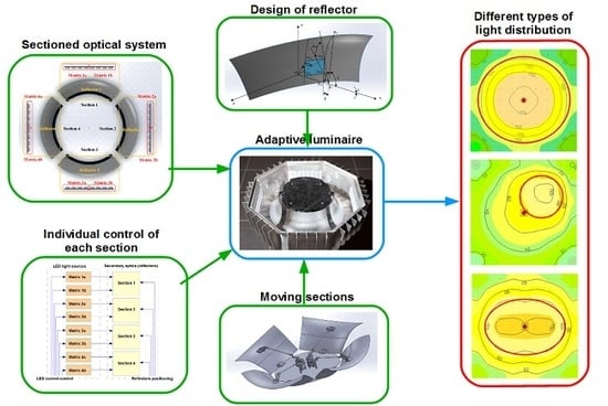
Considering the above, the research on the modeling and construction of light-optical systems of luminaires seems purposeful. The authors’s approach to the control of luminous intensity distribution differs from currently used design solutions. The aim of the study was to analyze the possibilities of forming a spatial distribution of light in a way that allows dynamic change of the shape of the solid of light distribution by means of appropriate optical elements, without the necessity of replacing them. Also, it provides rotationally symmetrical and bi-axially symmetrical distribution using the same optical system. The concept of an innovative luminaire was created, and preliminary simulation tests, which confirmed the assumptions, were conducted [28,29]. There were simulation works performed that only contained the possibility of luminous intensity distribution regulation by a designed optical system [28]. The next step was simulation studies but extended by analyzing lighting conditions on work surfaces with variable geometry and position [29]. The article presents the results of further studies, which include simulations as well as the construction and photometric measurements of a luminaire prototype. This solution can be used in smart lighting systems that adapt the way of lighting and the color of light to the shape and color of the illuminated object, for example, at an exhibition in shops or museums [30,31].
2. Luminaire Design Assumptions
A luminaire that would allow to quickly adjust the luminous intensity distribution to changing requirements on the working plane should provide the possibility of quantitative and directional adjustment of the emitted light. Therefore, the main design assumptions for a new type of luminaire were formulated:
- Adjustment of the luminous flux of light sources,
- Changing the luminous intensity distribution by positioning the elements of the optical system relative to the light source, without the necessity to replace them with elements with different geometry,
- Adjustment of luminous intensity distribution uniformly in all directions determined by the C half plane (Figure 4), with the rotational symmetry of the luminous intensity distribution maintained,
- Possibility of obtaining bi-axial luminous intensity distribution,
- Possibility of obtaining asymmetrical, diagonal distribution and directing it in one of eight main directions,
- The light-optical system consisting of independently controlled sections that enable the orientation of the light distribution in all directions,
- Ensuring adequate thermal conditions for the operation of LED sources in order to maintain high luminous efficacy.
3. Computer Modeling of the Light-Optical System of an Adaptive Luminaire
3.1. The Concept of the Optical System
The concept of forming the luminous intensity distribution changing dynamically during the operation of luminaire requires the use of movable elements of the optical system that change their position relative to the light source.
The use of LED sources allowed the use of lens systems due to their small dimensions. However, when the position of the lens relative to the LED source was changed in order to adjust the angle of light distribution, this solution proved to be ineffective due to the losses of luminous flux caused by the changed position of the lens and the consequent change of the amount of light radiated from a source and covered by the lens, as shown in Figure 5a,b.
In view of these problems, the use of a reflector for forming the luminous intensity distribution was considered. However, it was associated with a significant increase in the dimensions of the optical system. In addition, this solution does not give control over the direction of radiation of the entire luminous flux of the light source but only over a part of it, as shown in Figure 6.
A wide luminous intensity distribution of LED sources implies that the direction of radiation of a part of the luminous flux cannot be controlled. As a result, a part of the luminous flux is lost in the housing of the luminaire, and a part goes into space regardless of the position of reflector (direct component). This limits the possibility of narrowing the light distribution of the luminaire. For this reason, it was decided to use a hybrid solution that combines both types of optical systems.
A solution was devised that uses a movable reflector changing the final luminous intensity distribution of the luminaire, and the lens limiting the beam angle of light sources, and focusing the entire luminous flux on the reflector. It gives maximum control over the direction of light radiation and reduces losses. The method of forming the light distribution by means of a movable reflector at various angles of its inclination is shown in Figure 7a,b.
A complete luminaire consists of a set of light-optical elements that participate in the production of luminous flux (LED matrices) and forming its distribution characteristics (reflectors) by adjusting the operating parameters such as the position of the reflectors and the power of the sources. The structure of the control system of the designed luminaire is shown in Figure 8.
The entire light-optical system is divided into four main sections, as shown in Figure 9. Each section consists of a matrix of LED sources equipped with lenses constituting the primary optical system in which the task is to narrow the distribution of light sources and direct the luminous flux towards the secondary optical system, i.e., towards the reflector. Each of the LED matrices is divided into two independently powered subsections, which allows greater possibilities of shaping the asymmetrical distribution. The secondary optical system is an element changing the position by rotation about a horizontal axis passing through its base. This allows changing the direction of light radiation from the luminaire, which changes the beam angle. The division of the light-optical system into sections makes it possible to control the light distribution symmetrically, asymmetrically, and independently of each other, which allows the beam angle to be extended or narrowed only on one side, in the longitudinal, transverse, or diagonal axis.
The light distribution of the luminaire is caused by the movement of the reflector relative to the light source. The movement is executed by turning the reflector around an axis passing through its base, in the middle, or upper part of the focusing profile. In the adopted concept, the light source is placed on a vertical plane. The reflector changes its position by rotating around an axis passing through its base. This type of movement results from the need to place all optical elements inside a closed luminaire. The widest range of reflector’s movement is achieved by positioning the rotation axis at the base. The manner of movement is presented in Figure 10. The maximum inclination of the reflector towards the source matrix is the position where its upper edge remains above the upper edge of the matrix. This ensures that the reflector covers the luminous flux of the sources. Therefore, it was assumed that the critical angle of the reflector inclination was 20°. The movement of reflectors is provided through the motorized arms, as shown in Figure 11.
3.2. Modeling the Surface of Reflector
Determining the shape of the reflector, which implements the desired distribution, is a complex issue to which the analytical and graphic methods can be used [32,33].
The surface of the reflector of any shape with a parabolic profile can be mapped in a point or mesh manner. The vertices of the mesh surface lie on the surface, which is created by rotating around Oy axis or pulling the profile that is a part of the parabola located in the Oxy plane along Oz axis, as shown in Figure 12. Several methods that allow plotting points lying on the profile curve are known [34,35]. If a parabolic profile is used, it can be assumed that radial-angular division will be the most appropriate. It provides uneven distribution of points on the parabola with more points in the vertex zone, and fewer points in the zone of the parabola arms. It results from higher, and lower accuracy of profile mapping in individual zones. It is caused by more frequent occurrence of multiple reflections in the area of the parabola vertex.
In order to describe the mathematical parabolic profile, in the assumed system of coordinates, it is necessary to define the focal point Fl(xF,O), the axis of radiation of the light beam reflected from the reflector’s surface (determined by ν angle measured from the Ox axis), reflector’s cover angle (included between the sections FlPO i FlPN), and a point on the edge of the reflector PO(xO,yO). Parabola is approximated by replacing the curve with straight sections at a given angular division specified by the nO parameter.
In order to simplify the notation, the following designations have been adopted:
Hence the equation of parabola takes the following form:
The focal length of the parabola is defined by the relationship:
and the condition
is additionally satisfied.
If the described parabola is rotated around the Oy axis, a rotational surface is obtained, and its vertex points can be described in the form of a matrix:
where: oraz .
Oij = [Oij],
The matrix (5) is obtained by assigning new points lying in the plane Oxz to points Pi, using a constant of angular division mO, the number of new points being , (K ∈ N).
The authors developed the reflector profile that, for the assumed dimensions, and the range of movement, allows the change of the beam angle of rotationally symmetrical distribution in the range between 80–125°. The final shape of the reflector is shown in Figure 13. The reflector focusing profile consists of two parabolic curves.
The upper profile curve reflects the rays of the light source over the entire angle range from 0 degrees to the maximum luminous intensity angle for the reflector inclination set to 0°. The lower profile curve is optimized for a narrow range of angles, close to the maximum luminous intensity angle, in order to increase the maximum luminous intensity over the entire range of reflector inclination.
3.3. Analysis of Optically Active Reflector Surface
The luminous intensity distribution depends on many factors, such as geometry or physical properties of materials used to manufacture elements of the optical system. In the case of the reflector, which is the main element responsible for forming the light distribution in the designed luminaire, the shape of the focusing profile plays a decisive role, but the distribution also depends on the material used, and its reflective properties. Three main types of light reflection are distinguished: directional, diffuse, and directional-diffuse. The type of reflection depends on the surface of the material used: mirror, diffusing, or with a diffusing macrostructure. The reflectors made of these materials are offered by various manufacturers [36,37,38]. The selection of material, ensuring an appropriate degree of light focusing or scattering, is particularly important in the case of a movable reflector as its position shapes either a wide or focused distribution.
The basic reflector material is a material with a mirror surface that provides directional reflection. In the proposed design, the material did not fulfill its task due to uneven luminous intensity distribution at wide distribution and consequent underexposure in the axis of the luminaire. Examples of luminous intensity curves for the two extreme distributions of a luminaire with a mirror reflector are shown in Figure 14.
The diffusing material, causing Lambertian reflection, did not provide sufficient adjustability of light distribution in the designed solution due to too small orientation of reflection causing the insufficient focus of the light beam at narrow distribution. Examples of luminous intensity curves for the two extreme distributions of a luminaire with a diffuse reflector are shown in Figure 15.
The next tested solution is a material with a surface that provides directional-diffuse reflection. The analysis of materials with varying levels of diffusion was conducted by proper matting of the active surface. However, the available materials of this type were characterized by too high a degree of diffusion, which made the required adjustability of distribution impossible. Therefore, the materials with a mirror surface with a diffusing macrostructure were tested. Examples of luminous intensity curves for the two extreme distributions of a luminaire with a mirror surface with a diffusing macrostructure are shown in Figure 16.
4. Testing the Performance of Optical System
4.1. Constructing a Luminaire Prototype
Due to technological difficulties connected with shaping the reflector curvature from structural materials in the pressing process, the reflector for the developed prototype was made in 3D printing technology. The active surface of the reflector was covered with a concave honeycomb structure similar to that of the material used at an earlier stage of simulations. The view of the element with the structure applied is shown in Figure 17.
The next stage was constructing the luminaire prototype and determining its luminous intensity curves on the basis of measurements. The reflector model was made by a 3D printing method and had its surface sputtered with a metallic layer to obtain reflection properties. The finished object is shown in Figure 18. In the luminaire, the reflectors were mounted on joints, which enable their movement in relation to light sources.
A view of the complete prototype luminaire is shown in Figure 19.
The luminaire was equipped with 64 XP-G3 LED sources with a maximum power of 6 W [39]. Under normal operating conditions, the power of the source is 3 W, which gives a total rated power of 192 W. The power reserve allows, if necessary, to increase the power in one section, while reducing it in another, so as not to exceed the maximum power of the luminaire, i.e., 200 W. The C14607_HB-2X2-M type lenses installed on the XP-G3 source have a distribution angle of 28 degrees [40].
4.2. Determining Luminous Intensity Distribution
In order to verify whether the assumed types of distribution can be obtained the computer, simulations were performed to determine luminaire’s luminous intensity curves for luminaire supplied with rated power. The computations of luminous intensity distribution were conducted for the geometric model of the reflector presented in Figure 17. The model was used to construct a prototype of the luminaire. Photopia software (version 2019, LTI Optics, LLC, Westminster, CO, USA) was employed for computations [41].
The real luminous intensity distributions were determined, at rated power, for three characteristic options of rotationally symmetrical distribution: in reflector’s two extreme adjustable positions, and in the intermediate position. These options were selected because they give the possibility to precisely set the inclination angle of the reflectors in the appropriate position relative to the light sources in the range from 0 to 20°. The comparison of luminous intensity curves was made only for rotationally symmetrical distributions, with the exception of asymmetrical options, because luminous intensity curves obtained in rotationally symmetrical options are components of asymmetrical options in characteristic half planes. The luminous intensity curves were determined with a uniform angular step over the entire measuring range, which results from the fact that the expected luminous intensity curve does not have large gradients, and the light beam is relatively wide. In the case of a very narrow light beam, the number of measurements of directional flux should be increased, and decreased in particular zones. This principle is applied, for example, in signal lighting [42].
The comparison of luminous intensity curves obtained in simulations, and by prototype measurements is shown in Figure 20, Figure 21 and Figure 22. The luminous intensity curves obtained in simulations and measurements for wide distribution are similar to each other for the range of angles greater than the angle of maximum luminous intensity. The differences are bigger in the range from maximum luminous intensity to axial luminous intensity. The luminous intensity curves for medium distribution have a shape, and values that are more similar for individual angles. They are similar to the curves for narrow distribution.
The values of maximum luminous intensity in all analyzed cases differ from each other by less than 5%. Their curves depending on the angle of inclination of the reflectors are shown in Figure 23. The values of maximum luminous intensity for wide distribution are achieved at slightly different angles. In turn, the beam angles differ by no more than 3.5% in the case of wide and medium distribution, whereas for narrow distribution, the difference is bigger and amounts to 10%; however, it is still at an acceptable level. The change of beam angle depending on the inclination angle of reflectors is shown in Figure 24.
4.3. Determining Illuminance on the Plane
In the next step, made in order to compare and verify the compatibility of the prototype with the simulation model, the shape of the obtained light spots and the illuminance distribution on the plane were compared. Figure 25, Figure 26, Figure 27 and Figure 28 present the comparison of the illuminance distribution on the plane determined by the measurements of prototype’s luminous intensity distributions with the distributions obtained on the basis of luminous intensity distributions determined by simulation of the developed system. Illuminance distributions were determined for the 10 by 10 m plane, and the luminaire suspended 4 m above the plane, using the DIALux evo software (version 8.1, DIAL GmbH, Luedenscheid, Germany) [43]. The position of the luminaire relative to the illuminated plane is constant, and the positioning of individual reflector sections relative to light sources changes in the range from 0 to 20o. Red points in the figures indicate the center of the computational plane through which the luminaire’s optical axis passes, and the circles indicate the approximate shape of the light spot.
Figure 25 presents the illuminance distribution on a plane illuminated by a luminaire with a wide rotationally symmetrical distribution. Both in the simulation (Figure 25a) and in the real option (Figure 25b) can distinguish the area where the illuminance assumes values are not smaller than 100 lx. This area is approximated with a circle with a diameter of 9 m (red circles in Figure 25). While comparing the distribution of isolines with higher values, a certain asymmetry for the real option is observed. It may be caused by an imprecise production process of reflectors.
Illuminance distributions for narrow light distribution are shown in Figure 26. In both cases, similar results were obtained, 100 lx in an area with a diameter of 8 m, 300 lx in an area with a diameter of approximately 3 m, and over 500 lx in the center of the computation plane. A slight asymmetry of distribution can be noticed for the prototype.
The first of the asymmetrical options assumes the shift of a narrowed light spot in one axis, as shown in Figure 27.
The center of the area with a diameter of 4 m and illuminance above 200 lx is shifted relative to the plane center by 1 m in the transverse axis. In the option with the real luminaire, this area has a more oval shape than in the simulation.
In the second option, a diagonal (bi-axial) shift of a narrowed light spot was obtained, and the illuminance distribution is shown in Figure 28. In the simulation option, the area with illuminance above 80 lx has a diameter of 3 m, and for a real luminaire, it is about 3.5 m. In both cases, the shift of the center of the light spot relative to the plane center is approximately 2 m.
In the third option, the distribution with two symmetry axes, narrowed in one axis and similar to linear distribution, is obtained. The illuminance distribution is shown in Figure 29. The area with illuminance above 120–125 lx is oval shaped and measures 8 by 4 m in the case of simulation, and in the case of a real luminaire, its width decreases to approximately 3.5 m.
4.4. Analysis of Optical Efficiency
The ability to adjust the beam angle of the luminaire carries the complication of the optical system, which can cause additional luminous flux losses, and thus also power losses. Figure 30 shows the change in luminous flux as a function of beam angle, and the luminaire was supplied at constant power. The luminous flux of the sources is constant, while at the luminous flux opening the luminaire changes at different beam angles. The maximum value occurs in the middle of the range of the beam angle changes and the minimum values at its ends. The difference between the maximum and minimum value is less than 3.5%.
Figure 31 shows changes in the optical efficiency of the luminaire as a function of changes in the beam angle. The efficiency curve is analogous to changes in the light output from the luminaire. The efficiency varies from 72.5% to 75%. The smallest value occurs at the widest distribution.
The optical efficiency of other luminaires with adjustable light distribution, for example, luminaires shown in Figure 3, can be used as a reference for assessing optical efficiency. They are characterized by a narrow light beam and use a different type of optical system. The luminaire from Figure 3a with a power of 3 W has an angle adjustment range from 14 to 34 degrees and has an optical efficiency of about 32%. In turn, the luminaire shown in Figure 3b with a power of 26 W allows to adjust the beam angle in the range of 16 to 42 degrees, its optical efficiency varies in the range of 42% to 48%. It can be seen that the developed luminaire is characterized by a clearly higher optical efficiency (72%–75%), which is particularly important due to the higher power level (192 W).
5. Conclusions
Considering the results obtained by comparing the luminous intensity distribution (LID) curves of the prototype and the simulation model, it can be concluded that the compatibility of results confirms the assumed possibility of adjusting the luminous intensity distribution in the angle range between approximately 80 and 125 degrees. Based upon the comparison of light spots and illuminance distribution, determined with the use of luminous intensity distributions obtained in computer simulations, with the LIDs measured on the luminaire prototype, it should be noted that light spots show significant similarities of characteristic areas both in terms of shape and illuminance values. Some differences in the shape of the illuminated area, which are most likely due to the inaccuracy of prototype components, can be seen.
Thanks to the use of reflectors as elements responsible for adjusting the beam angle, the luminaire is characterized by higher optical efficiency than luminaires with adjustable distribution, which use lens optics. By limiting the loss of luminous flux in the optical system, it is possible to design luminaires with adjustable distribution and high power, comparable to industrial luminaires.
The obtained results allow to state that the developed luminaire meets the main constructional assumptions of adaptive distribution, including symmetrical change of the beam angle and the possibility of forming the asymmetrical distribution. More refined technology of manufacturing individual elements of the luminaire, mainly reflectors, as well as the improvement of their positioning precision, should allow for even greater compatibility of the real luminaire with the simulation model. At the same time, further works on the development of luminaires are conducted. They focus on the source control system, the positioning of reflectors, and the integration with adaptive lighting control systems.
The developed luminaire, due to its properties, can be used in both general and local lighting in facilities with a large usable space. In cooperation with smart lighting systems, it can be used to dynamically create a lighting scene, for example, displays in shops, museums, exhibition centers. The luminaire with variable light distribution is a solution that saves time and money needed to modernize lighting where space arrangement often changes, due to the fact that the installation works must be done once. It is estimated that the cost of a new luminaire will be about 30%-40% higher than a classic luminaire with comparable power with adjustable luminous flux, due to the more complex construction. However, the savings are expected if any changes in lighting are planned during exploitation.
Author Contributions
Measurements of luminaire’s luminous intensity distribution were made by H.W. and M.L. The results of studies presented in this manuscript and their assessment was carried out by M.L. and A.R. Finally, M.L., H.W., and S.R. supervised the research and prepared the manuscript. All authors have read and agreed to the published version of the manuscript.
Funding
This research received no external funding.
Conflicts of Interest
The authors declare no conflict of interest.
References
- Khanh, T.; Bodrogi, P.; Vinh, Q.; Winkler, H. LED Lighting. Technology and Perception; Wiley-VCH Verlag GmbH: Darmstadt, Germany, 2015. [Google Scholar]
- Różowicz, A.; Leśko, M.; Wachta, H. Evaluation of the zonal luminous flux distribution of LED sources. In Proceedings of the 2016 13th Selected Issues of Electrical Engineering and Electronics (WZEE), Rzeszow, Poland, 4–8 May 2016; pp. 1–6. [Google Scholar]
- Barbosa, J.L.F.; Simon, D.; Calixto, W.P. Design Optimization of a High Power LED Matrix Luminaire. Energies 2017, 10, 639. [Google Scholar] [CrossRef] [Green Version]
- Barbosa, J.L.F.; Calixto, W.P.; Simon, D. High power LED luminaire design optimization. In Proceedings of the IEEE 16th International Conference on Environment and Electrical Engineering, Florence, Italy, 7–10 June 2016; pp. 1–6. [Google Scholar]
- Rozowicz, A.; Lesko, M.; Wachta, H. The technical possibilities of losses reduction in the LED optical systems. In Proceedings of the 2016 IEEE Lighting Conference of the Visegrad Countries (Lumen V4), Karpacz, Poland, 13–16 September 2016; pp. 1–5. [Google Scholar]
- Vu, N.H.; Tuan Pham, T.; Shin, S. LED Uniform Illumination Using Double Linear Fresnel Lenses for Energy Saving. Energies 2017, 10, 2091. [Google Scholar] [CrossRef] [Green Version]
- Light and Lighting—Lighting of Work Places—Part 1: Indoor Work Places; EN 16464-1: 2012; PKN: Warszawa, Poland, 2012; Polish Version.
- CIE. Review of Lighting Quality Measures for Interior Lighting with LED Lighting Systems; Technical Report 205:2013; CIE: Vienna, Austria, 2013. [Google Scholar]
- Guideline for the Application of General Illumination (“White”) Light-Emitting Diode (LED) Technologies; IES G-2-10; Illuminating Engineering Society: New York, NY, USA, 2010.
- Liu, M.; Rong, B.; Salemink, H.W. Evaluation of LED application in general lighting. Opt. Eng. 2007, 46, 074002. [Google Scholar]
- Gueorgiev, V.; Rizov, P. Lighting in High Temperature Industrial Enviroment. In Proceedings of the 2018 Seventh Balkan Conference on Lighting (BalkanLight), Varna, Bulgaria, 20–22 September 2018; pp. 1–3. [Google Scholar]
- Barroso, A.; Dupuis, P.; Alonso, C.; Jammes, B.; Seguier, L.; Zissis, G. A characterization framework to optimize LED luminaire’s luminous efficacy. In Proceedings of the 2015 IEEE Industry Applications Society Annual Meeting, Addison, TX, USA, 18–22 October 2015; pp. 905–913. [Google Scholar]
- Baran, K.; Wachta, H.; Leśko, M.; Różowicz, A. Research on thermal resistance Rthj-c of high power semiconductor light sources. In Proceedings of the 15th Conference on Computational Technologies in Engineering, Mikolajki, Poland, 16–19 October 2018; AIP Conference Proceedings 2078. p. 020047. [Google Scholar]
- Baran, K.; Wachta, H.; Leśko, M.; Różowicz, A. Thermal Modeling and Simulation of High Power LED Module. In Proceedings of the 15th Conference on Computational Technologies in Engineering, Mikolajki, Poland, 16–19 October 2018; AIP Conference Proceedings 2078. p. 020048. [Google Scholar]
- Lasance, C.; Poppe, A. Thermal Management for LED Applications; Springer Science, Business Media: New York, NY, USA, 2014. [Google Scholar]
- Mathews, E.; Guclu, S.S.; Liu, Q.; Ozcelebi, T.; Lukkien, J.J. The Internet of Lights: An Open Reference Architecture and Implementation for Intelligent Solid State Lighting Systems. Energies 2017, 10, 1187. [Google Scholar] [CrossRef] [Green Version]
- Vu, N.H.; Shin, S. Flat Optical Fiber Daylighting System with Lateral Displacement Sun-Tracking Mechanism for Indoor Lighting. Energies 2017, 10, 1679. [Google Scholar] [CrossRef] [Green Version]
- Scientific Committee on Health, Environmental and Emerging Risks (SCHEER). Opinion on Potential risks to human health of Light Emitting Diodes (LEDs); SCHEER: Bruxelles, Belgium, 2018. [Google Scholar]
- Behar-Cohen, F.; Martinsons, C.; Viénot, F.; Zissis, G.; Barlier-Salsi, A.; Cesarini, J.P.; Enouf, O.; Garcia, M.; Picaud, S.; Attiah, D. Light-emitting diodes (LED) for domestic lighting: Any risks for the eye? Prog. Retin. Eye Res. 2011, 30, 239–257. [Google Scholar] [CrossRef] [PubMed]
- Leccese, F.; Salvadori, G.; Casini, M.; Bertozzi, M. Analysis and Measurements of Artificial Optical Radiation (AOR) Emitted by Lighting Sources Found in Offices. Sustainability 2014, 6, 5941–5954. [Google Scholar] [CrossRef] [Green Version]
- Photobiological Safety of Lamps and Lamp Systems; IEC/EN 62471: 2006; IEC: Geneva, Switzerland, 2006.
- Photobiological Safety of Lamps and Lamp Systems. Part 2: Guidance on Manufacturing Requirements Relating to Non-Laser Optical Radiation Safety; IEC/TR 62471-2:2009; IEC: Geneva, Switzerland, 2009.
- Application of IEC 62471 for the Assessment of Blue Light Hazard to Light Sources and Luminaires; IEC/TR 62778:2014; IEC: Geneva, Switzerland, 2014.
- SOLLS Products. Available online: http://solls.pl/katalog/produkty/ (accessed on 12 November 2019).
- ES-System Industry Flower. Available online: https://www.essystem.pl/produkty/s/59;industry-flower-maxi (accessed on 12 November 2019).
- Targetti Otto. Available online: http://www.targetti.com/en/indoor-lighting/projectors/otto_base (accessed on 16 December 2019).
- Targetti Zeno Medium DBS. Available online: http://www.targetti.com/en/indoor-lighting/projectors/zeno/?0=Reflector||168||DBS (accessed on 16 December 2019).
- Leśko, M.; Różowicz, A.; Baran, K.; Wachta, H. A luminaire with variable light distribution. E3S Web Conf. 2018, 49, 00066. [Google Scholar] [CrossRef] [Green Version]
- Leśko, M.; Baran, K.; Wachta, H.; Różowicz, A. A Concept of an Adaptive Luminaire with Variable Luminous Intensity Distribution. In Proceedings of the 2018 VII Lighting Conference of the Visegrad Countries (Lumen V4), Trebic, Czech Republic, 18–20 September 2018; pp. 1–4. [Google Scholar]
- Durmus, D.; Davis, W. Optimising light source spectrum for object reflectance. Opt. Express 2015, 23, A456–A464. [Google Scholar] [CrossRef] [PubMed]
- Vázquez, D.; Alvarez, A.; Canabal, H.; Garcia, A.; Mayorga, S.; Muro, C.; Galan, T. Point to point multispectral light projection applied to cultural heritage. In Proceedings of the SPIE 10379, Nonimaging Optics: Efficient Design for Illumination and Solar Concentration XIV, San Diego, CA, USA, 7 September 2017; p. 103790K. [Google Scholar]
- Elmer, W.B. The Optical Design of Reflectors; John Wiley &Sons: New York, NY, USA, 1980. [Google Scholar]
- Zalewski, S. A proposed method for the calculation of light emitting diode road lighting. Light. Res. Technol. 2012, 44, 186–196. [Google Scholar] [CrossRef]
- Januszewski, B.; Bieniasz, J. Geometryczne Podstawy Grafiki Inżynierskiej; Oficyna Wydawnicza Politechniki Rzeszowskiej: Rzeszów, Poland, 2000. (In Polish) [Google Scholar]
- Nicyporowicz, E. Krzywe płaskie. Wybrane Zagadnienia z Geometrii Analitycznej i Różniczkowej; PWN: Warszawa, Poland, 1991. (In Polish) [Google Scholar]
- Alanod. Available online: https://alanod-westlake.com/products/ (accessed on 12 November 2019).
- Almeco Group. Available online: https://almecogroup.com/en/pages/377-reflecting-surfaces-for-lighting (accessed on 12 November 2019).
- ACA Corp. Available online: https://acacorp.com/lighting/ (accessed on 12 November 2019).
- CREE LED Components. Available online: https://www.cree.com/led-components/products/xlamp-leds-discrete/xlamp-xp-g3 (accessed on 12 November 2019).
- LEDIL. Available online: https://www.ledil.com/product-card/?product=C14607_HB-2X2-M (accessed on 12 November 2019).
- LTI Optics Photopia Design Software. Available online: http://www.ltioptics.com/en/photopia-general-2017.html (accessed on 12 November 2019).
- Rozowicz, S.; Delag, M. Approval of Special Warning Lights for the Power-Driven Vehicles in Free Market. In Proceedings of the 2018 Conference: Conference on Electrotechnology–Processes, Models, Control and Computer Science (EPMCCS), Cedzyna, Poland, 12–14 November 2018. [Google Scholar]
- DIALux evo. Available online: https://www.dial.de/en/dialux-desktop/ (accessed on 12 November 2019).
Figure 1.
Large useable areas: (a) production hall, (b) storage hall.

Figure 2.
Selected luminaires with a rotationally symmetrical solid of light distribution and different type of optical system: (a) reflector type, (b) uncovered LED with optional diffusing glass, (c) lens type.
Figure 2.
Selected luminaires with a rotationally symmetrical solid of light distribution and different type of optical system: (a) reflector type, (b) uncovered LED with optional diffusing glass, (c) lens type.

Figure 3.
Selected luminaires with variable light beam opening: (a) manually controlled zoom lens, (b) aperture equipped with electronically controlled liquid crystal glass lenses.
Figure 3.
Selected luminaires with variable light beam opening: (a) manually controlled zoom lens, (b) aperture equipped with electronically controlled liquid crystal glass lenses.
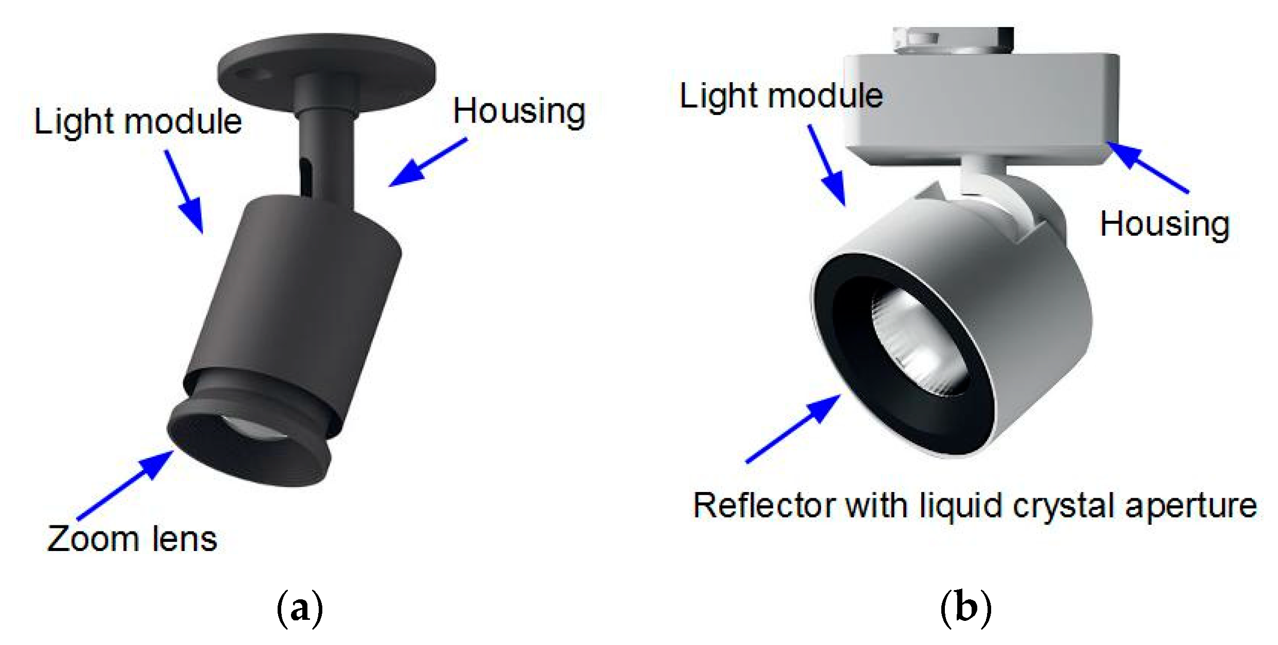
Figure 4.
The adjustment of light distribution angle in the C half plane.
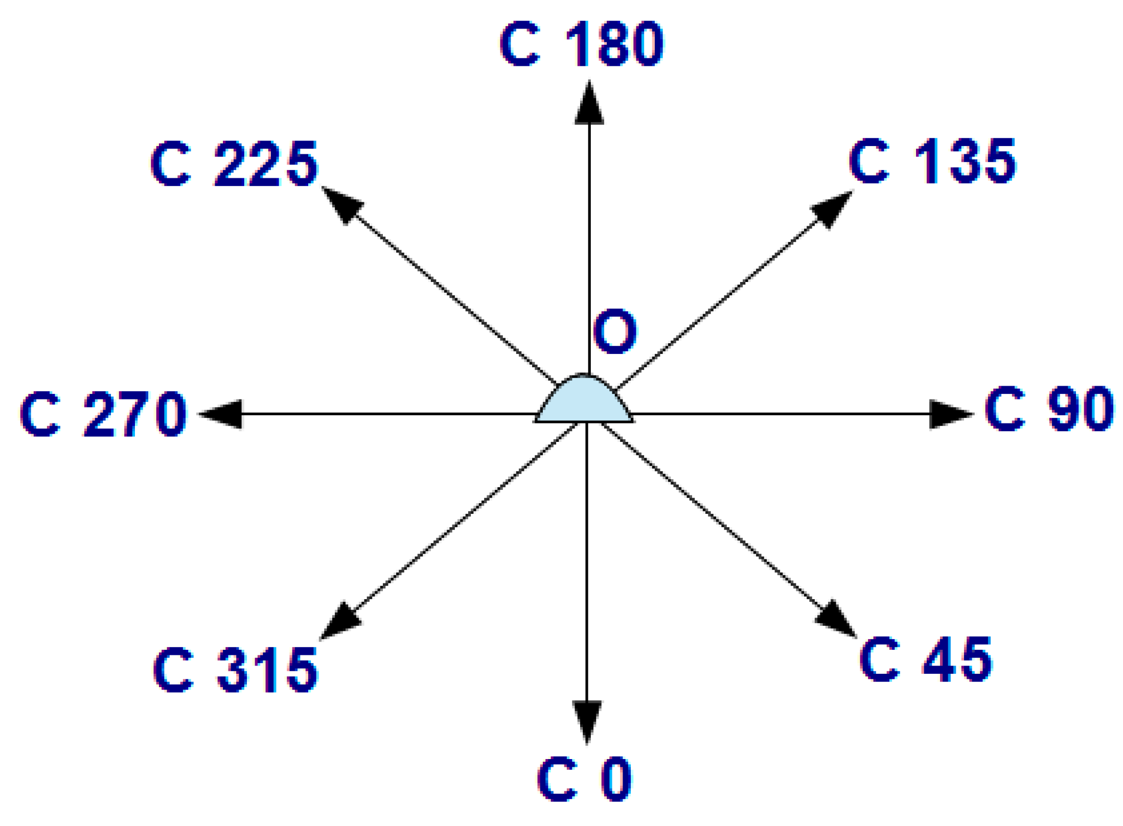
Figure 5.
The losses of luminous flux for the changed position of the lens relative to the LED source: (a) the lens positioned at a short distance from the source, (b) the lens positioned at a long distance from the source.
Figure 5.
The losses of luminous flux for the changed position of the lens relative to the LED source: (a) the lens positioned at a short distance from the source, (b) the lens positioned at a long distance from the source.

Figure 6.
Image of forming the luminous intensity distribution by a reflector system and the LED source without focusing lenses.
Figure 6.
Image of forming the luminous intensity distribution by a reflector system and the LED source without focusing lenses.
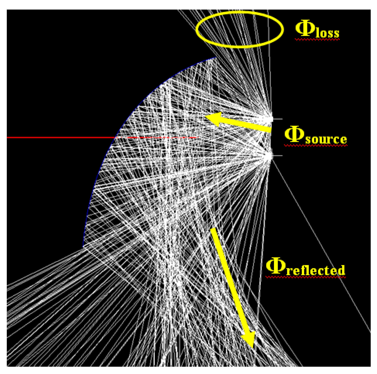
Figure 7.
Image of the change of a luminous flux direction for the changed inclination of the reflector relative to the LED light source with focusing lenses: (a) minimum inclination, (b) maximum inclination.
Figure 7.
Image of the change of a luminous flux direction for the changed inclination of the reflector relative to the LED light source with focusing lenses: (a) minimum inclination, (b) maximum inclination.
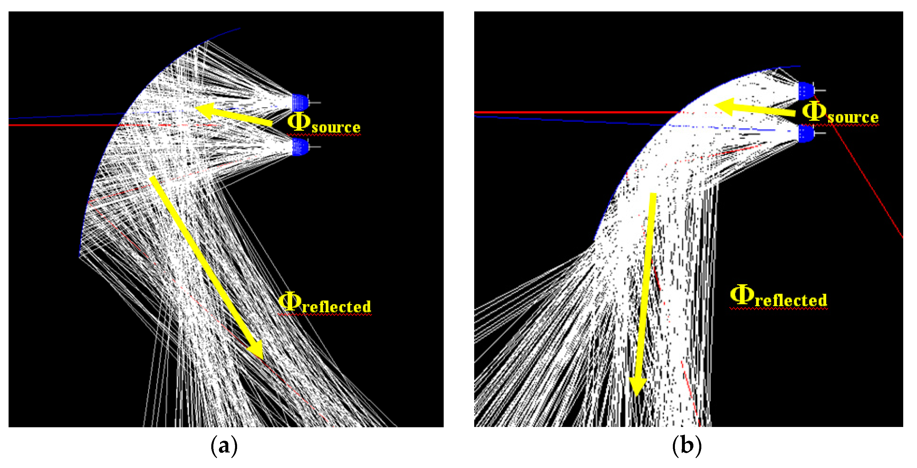
Figure 8.
Diagram of the luminaire’s control system.
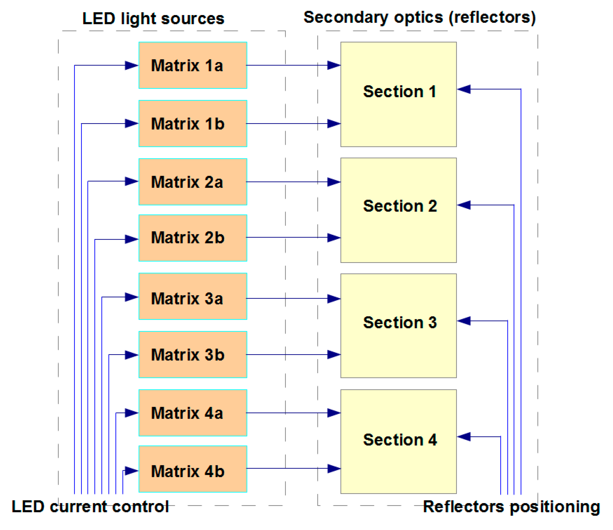
Figure 9.
The division of the light-optical system into sections.
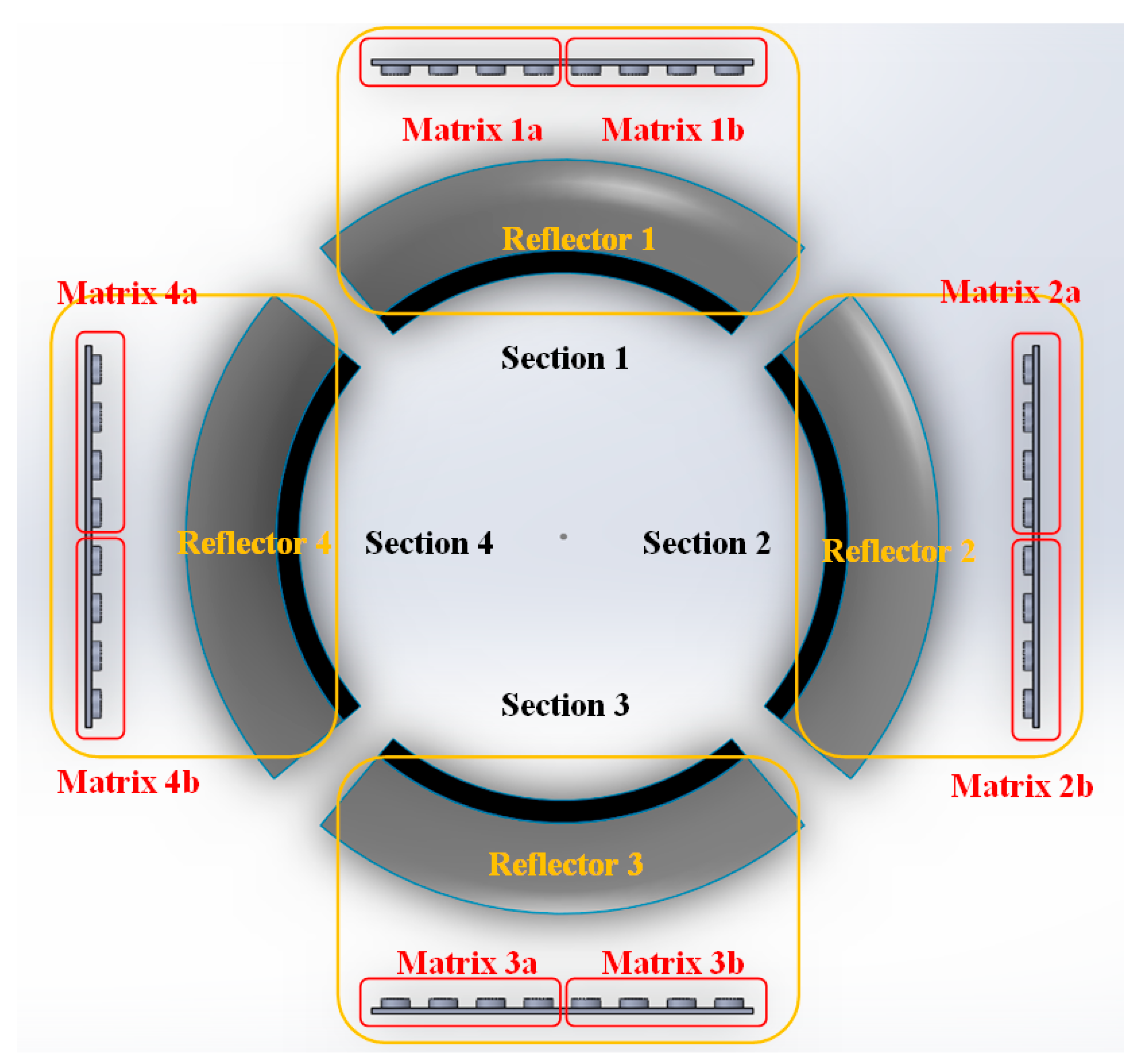
Figure 10.
The range of the angular movement of the reflector relative to the LED matrix: (a) minimum inclination, (b) maximum inclination.
Figure 10.
The range of the angular movement of the reflector relative to the LED matrix: (a) minimum inclination, (b) maximum inclination.

Figure 11.
The implementation of reflector movement using motorized arms.

Figure 12.
The geometric model of the reflector with the surface constituting a section of the parabolic torus, approximated by a set of finite number of elementary flat surfaces.
Figure 12.
The geometric model of the reflector with the surface constituting a section of the parabolic torus, approximated by a set of finite number of elementary flat surfaces.

Figure 13.
View of the reflector with a double-curved focusing profile.

Figure 14.
Luminous intensity curves for a luminaire with a mirror reflector: (a) wide distribution (b) narrow distribution.
Figure 14.
Luminous intensity curves for a luminaire with a mirror reflector: (a) wide distribution (b) narrow distribution.

Figure 15.
Luminous intensity curves for a luminaire with a diffuse reflector: (a) wide distribution (b) narrow distribution.
Figure 15.
Luminous intensity curves for a luminaire with a diffuse reflector: (a) wide distribution (b) narrow distribution.

Figure 16.
Luminous intensity curves for a reflector with a mirror surface and a diffusing macrostructure: (b) wide distribution (b) narrow distribution.
Figure 16.
Luminous intensity curves for a reflector with a mirror surface and a diffusing macrostructure: (b) wide distribution (b) narrow distribution.
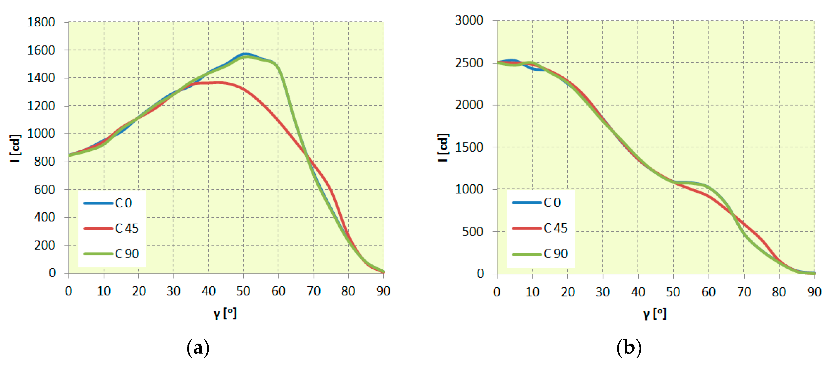
Figure 17.
View of the reflector model with a diffusing macrostructure.

Figure 18.
View of the finished reflector with a diffusing macrostructure and a metallic layer sputtered on it.
Figure 18.
View of the finished reflector with a diffusing macrostructure and a metallic layer sputtered on it.

Figure 19.
View of a complete prototype luminaire: (a) bottom with optical system, (b) top with radiator.
Figure 19.
View of a complete prototype luminaire: (a) bottom with optical system, (b) top with radiator.

Figure 20.
The comparison of luminous intensity curves of a light-optical system for wide distribution obtained as a result of simulation and prototype measurements.
Figure 20.
The comparison of luminous intensity curves of a light-optical system for wide distribution obtained as a result of simulation and prototype measurements.

Figure 21.
The comparison of luminous intensity curves of a light-optical system for medium wide distribution obtained as a result of simulation and prototype measurements.
Figure 21.
The comparison of luminous intensity curves of a light-optical system for medium wide distribution obtained as a result of simulation and prototype measurements.
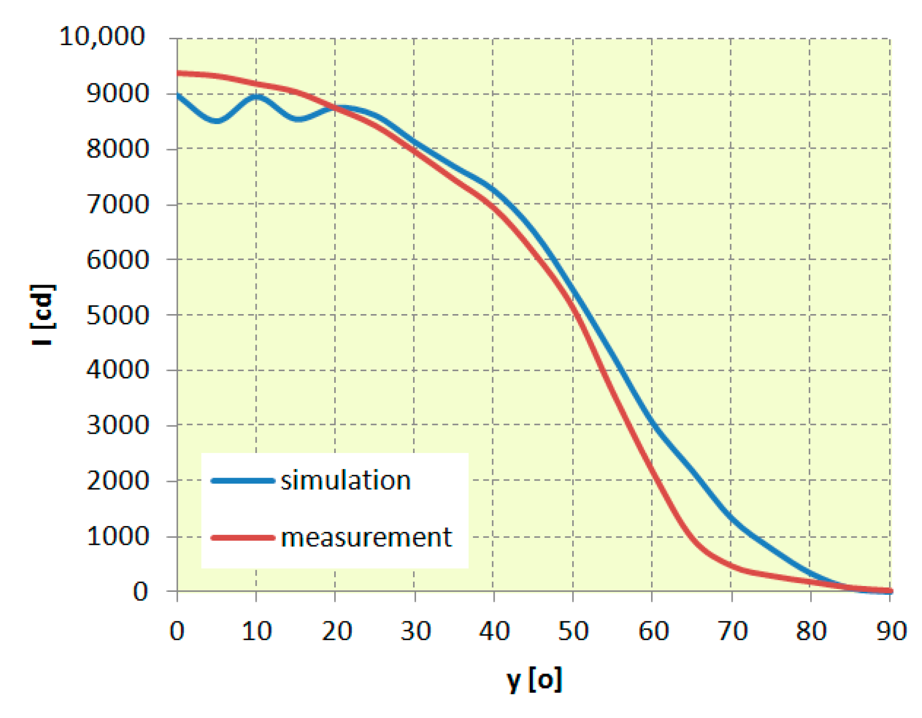
Figure 22.
The comparison of luminous intensity curves of a light-optical system for narrow distribution obtained as a result of simulation and prototype measurements.
Figure 22.
The comparison of luminous intensity curves of a light-optical system for narrow distribution obtained as a result of simulation and prototype measurements.
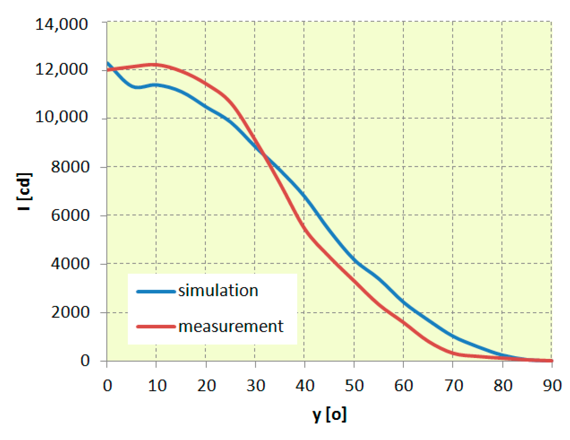
Figure 23.
The comparison of maximum luminous intensity of a light-optical system obtained as a result of simulation and prototype measurements in the function of reflector’s inclination angle.
Figure 23.
The comparison of maximum luminous intensity of a light-optical system obtained as a result of simulation and prototype measurements in the function of reflector’s inclination angle.

Figure 24.
The comparison of beam angles of a light-optical system obtained in simulations and by prototype measurements in the function of reflector’s inclination angle.
Figure 24.
The comparison of beam angles of a light-optical system obtained in simulations and by prototype measurements in the function of reflector’s inclination angle.
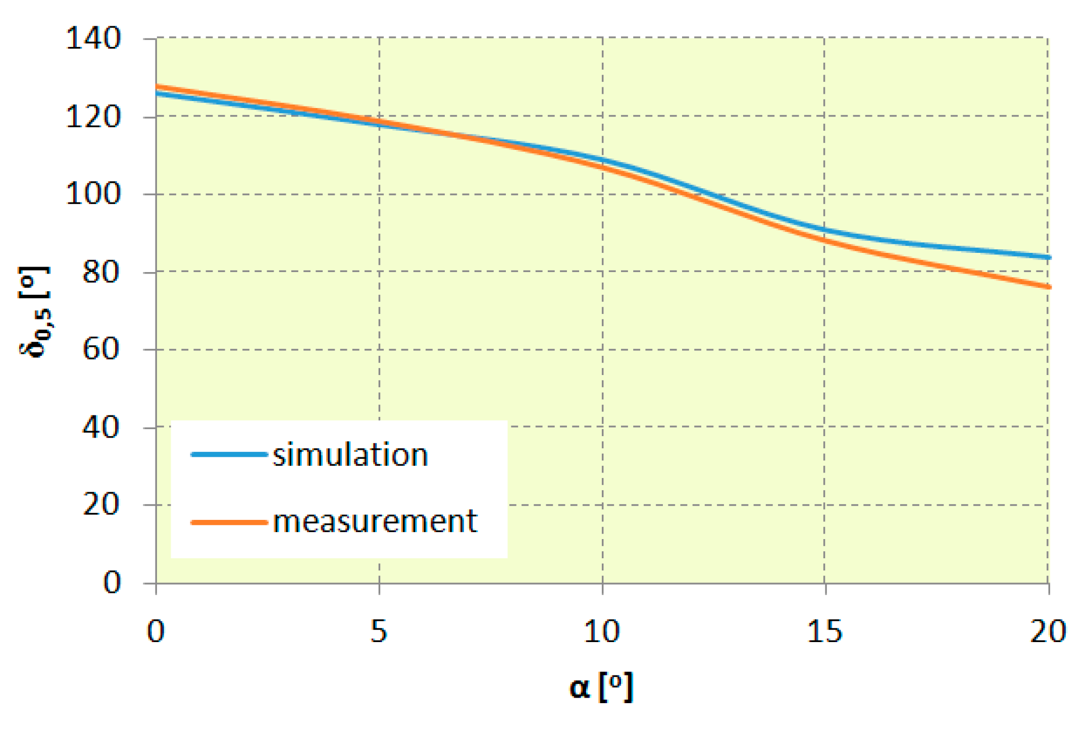
Figure 25.
Illuminance distribution on a plane for wide symmetrical light distribution (128°): (a) results for a simulation model, (b) results for a prototype luminaire.
Figure 25.
Illuminance distribution on a plane for wide symmetrical light distribution (128°): (a) results for a simulation model, (b) results for a prototype luminaire.
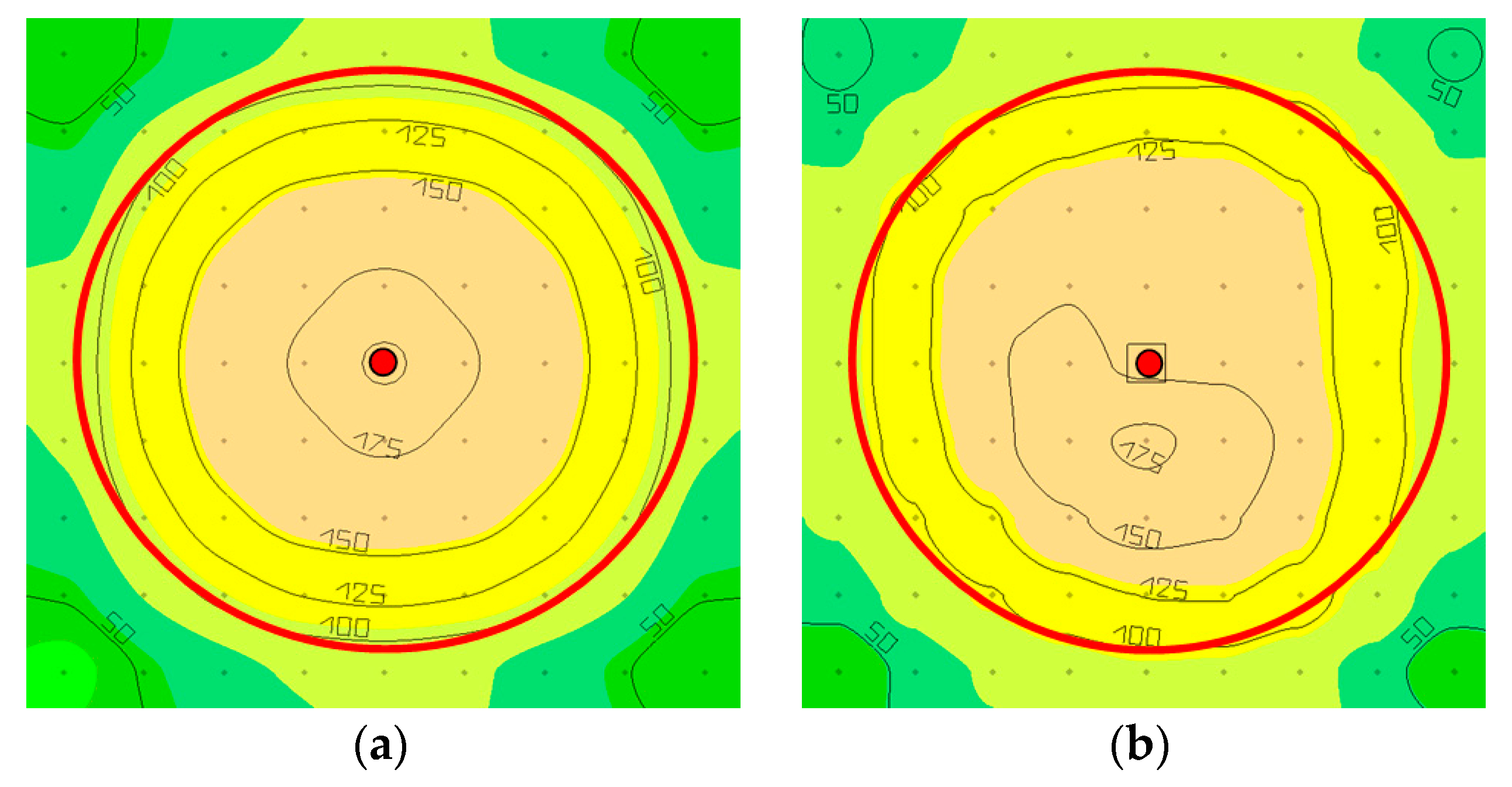
Figure 26.
Illuminance distribution on a plane for narrow symmetrical distribution (76°): (a) results for a simulation model, (b) results for a prototype luminaire.
Figure 26.
Illuminance distribution on a plane for narrow symmetrical distribution (76°): (a) results for a simulation model, (b) results for a prototype luminaire.
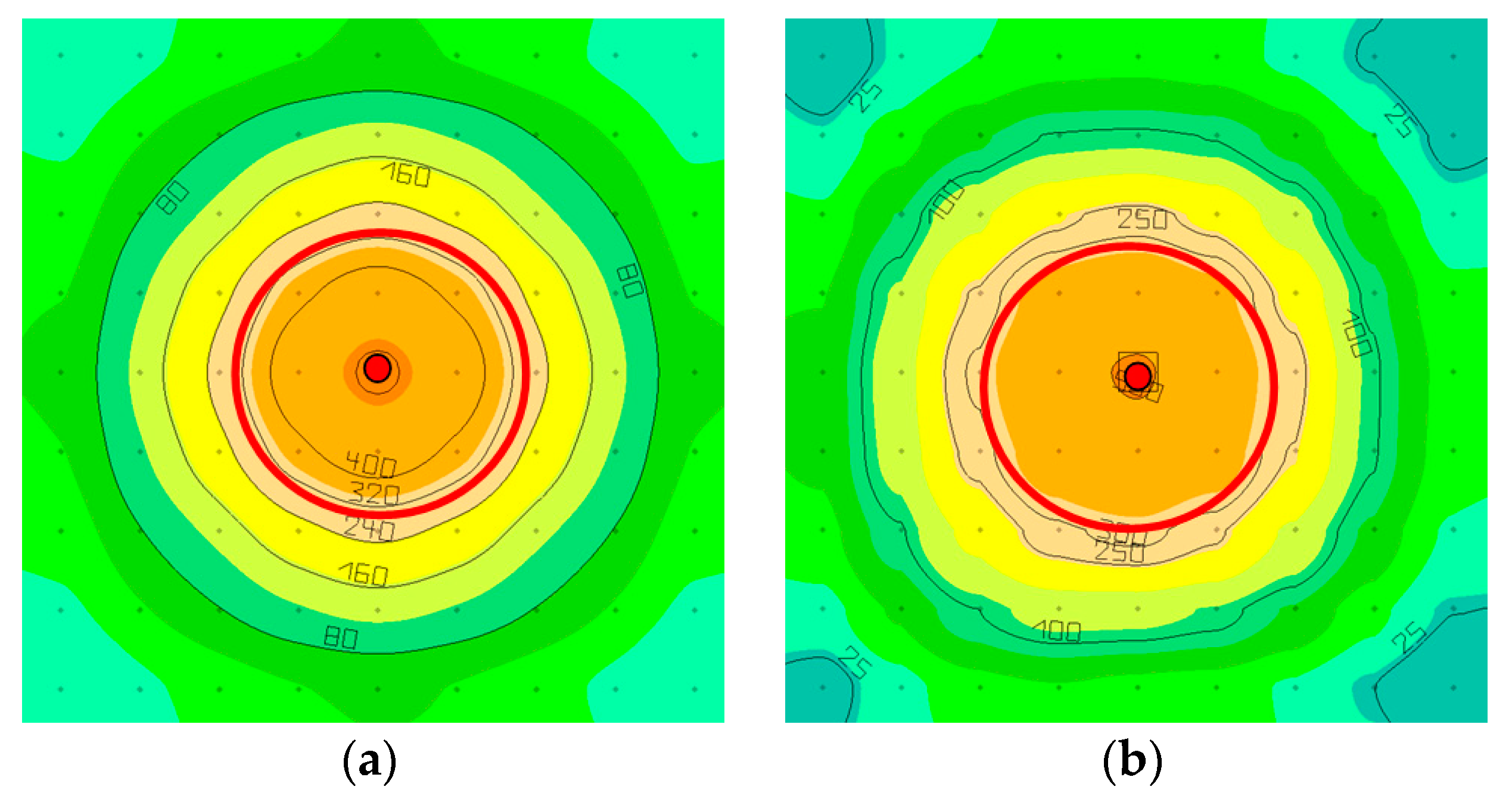
Figure 27.
Option 1, illuminance distribution on a plane for asymmetrical distribution (a) results for a simulation model, (b) results for a prototype luminaire.
Figure 27.
Option 1, illuminance distribution on a plane for asymmetrical distribution (a) results for a simulation model, (b) results for a prototype luminaire.
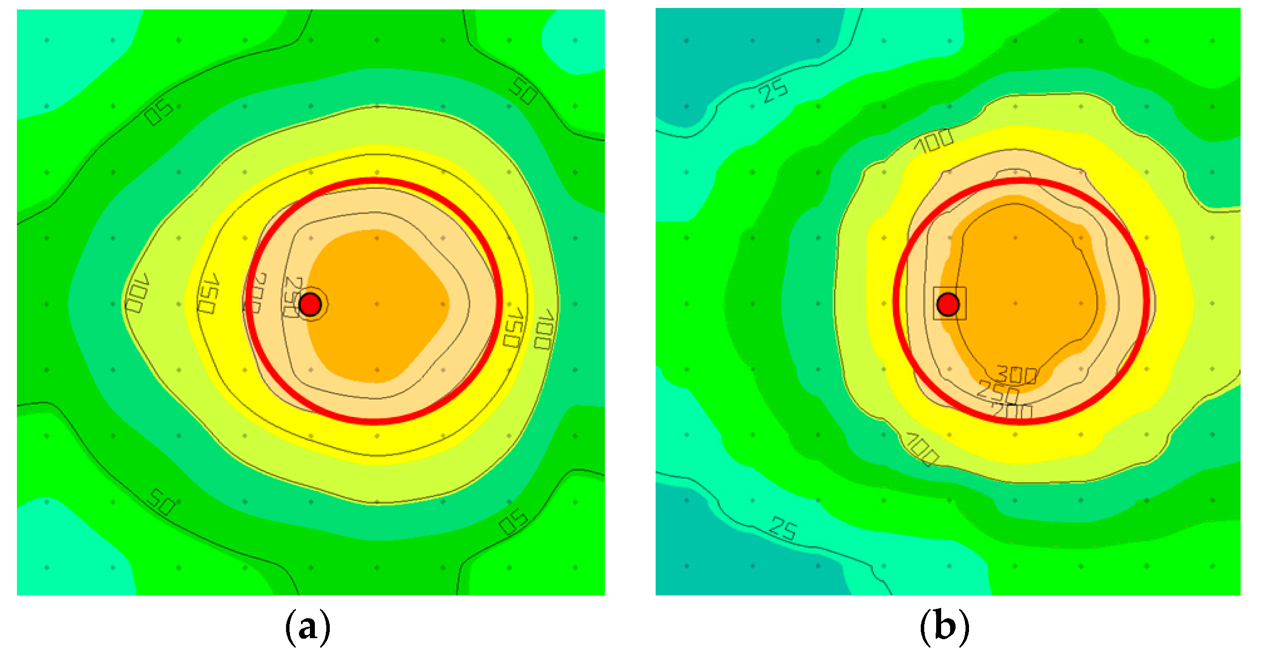
Figure 28.
Option 2, illuminance distribution on the plane for asymmetrical distribution (a) results for a simulation model, (b) results for a luminaire prototype.
Figure 28.
Option 2, illuminance distribution on the plane for asymmetrical distribution (a) results for a simulation model, (b) results for a luminaire prototype.
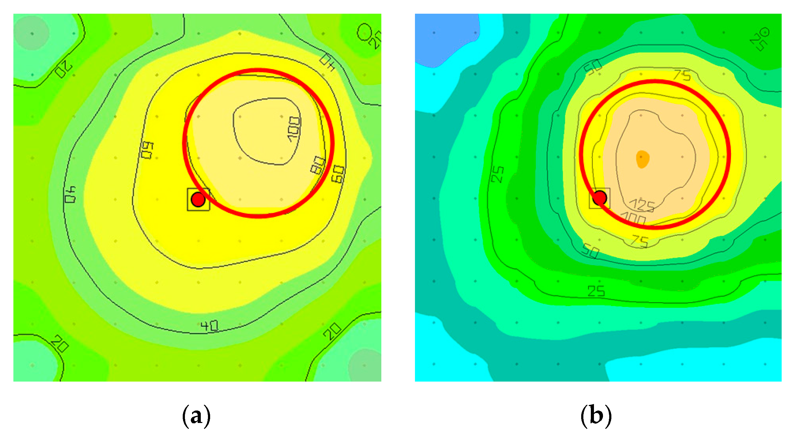
Figure 29.
Option 3, illuminance distribution on the plane for asymmetrical distribution (a) results for a simulation model, (b) results for a luminaire prototype.
Figure 29.
Option 3, illuminance distribution on the plane for asymmetrical distribution (a) results for a simulation model, (b) results for a luminaire prototype.

Figure 30.
Luminous flux as a function of beam angle.

Figure 31.
Optical efficiency of a luminaire as a function of beam angle.

© 2020 by the authors. Licensee MDPI, Basel, Switzerland. This article is an open access article distributed under the terms and conditions of the Creative Commons Attribution (CC BY) license (http://creativecommons.org/licenses/by/4.0/).
Share and Cite
MDPI and ACS Style
Leśko, M.; Różowicz, A.; Wachta, H.; Różowicz, S. Adaptive Luminaire with Variable Luminous Intensity Distribution. Energies 2020, 13, 721. https://doi.org/10.3390/en13030721
AMA Style
Leśko M, Różowicz A, Wachta H, Różowicz S. Adaptive Luminaire with Variable Luminous Intensity Distribution. Energies. 2020; 13(3):721. https://doi.org/10.3390/en13030721
Chicago/Turabian StyleLeśko, Marcin, Antoni Różowicz, Henryk Wachta, and Sebastian Różowicz. 2020. "Adaptive Luminaire with Variable Luminous Intensity Distribution" Energies 13, no. 3: 721. https://doi.org/10.3390/en13030721
Note that from the first issue of 2016, this journal uses article numbers instead of page numbers. See further details here.