A Study on Optimal Power System Reinforcement Measures Following Renewable Energy Expansion


1
School of Electrical Engineering, Daegu Catholic University, Gyeongsangbuk-do 38430, Korea
2
System Planning Department, KEPCO, Jeollanam-do 58322, Korea
*
Author to whom correspondence should be addressed.
Energies 2020, 13(22), 5929; https://doi.org/10.3390/en13225929
Submission received: 17 September 2020
/
Revised: 6 November 2020
/
Accepted: 7 November 2020
/
Published: 13 November 2020
(This article belongs to the Special Issue Modeling of Variable Renewable Generation: Wind and Solar Photovoltaic Power Plants)
Abstract
:Renewable energy generation capacity in Korea is expected to reach about 63.8 GW by 2030 based on calculations using values from a power plan survey (Korea’s renewable energy power generation project plan implemented in September 2017) and the “3020” implementation plan prescribed in the 8th Basic Plan for Long-Term Electricity Supply and Demand that was announced in 2017. In order for the electrical grid to accommodate this capacity, an appropriate power system reinforcement plan is critical. In this paper, a variety of scenarios are constructed involving renewable energy capacity, interconnection measures and reinforcement measures. Based on these scenarios, the impacts of large-scale renewable energy connections on the future power systems are analyzed and a reinforcement plan is proposed based on the system assessment results. First, the scenarios are categorized according to their renewable energy interconnection capacity and electricity supply and demand, from which a database is established. A dynamic model based on inverter-based resources is applied to the scenarios here. The transmission lines, high-voltage direct current and flexible alternating current transmission systems are reinforced to increase the stability and capabilities of the power systems considered here. Reinforcement measures are derived for each stage of renewable penetration based on static and dynamic analysis processes. As a result, when large-scale renewable energy has penetrated some areas in the future in Korean power systems, the most stable systems could be optimally configured by applying interconnection measure two and reinforcement measure two as described here. To verify the performance of the proposed methodology, in this paper, comprehensive tests are performed based on predicted large-scale power systems in 2026 and 2031. Database creation and simulation are performed semi-automatically here using Power System Simulator for Engineering (PSS/E) and Python.
1. Introduction
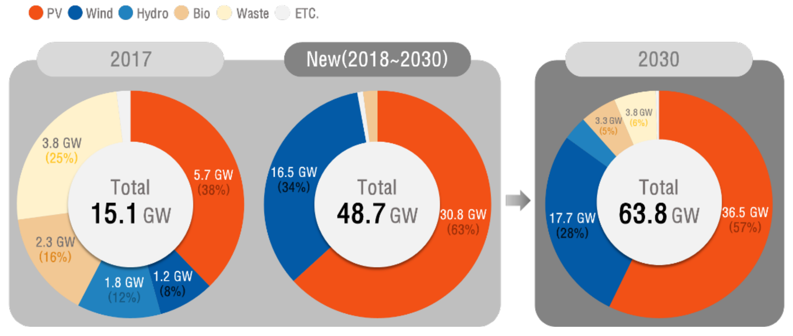
Increasing levels of carbon dioxide in the atmosphere have caused environmental problems, such as global warming, to worsen. In response, nations have created numerous environmental treaties. Since the signing of the Paris Agreement on Climate Change in 2015, countries worldwide have taken measures to reduce carbon dioxide levels in the atmosphere [1]. One such measure taken by power companies is adding natural gas generators and renewable energy generators, which rarely emit carbon, while reducing the number of carbon-emitting power generators like coal and thermal power plants, thereby contributing to the reduction of carbon dioxide emissions [2]. In line with this trend of energy conversion, Korea also has announced the “3020” Implementation Plan, which was revised recently. As such, Korea plans to construct 63.8 GW of renewable energy generation capacity by 2030, as shown in Figure 1. By 2030, the plan aims to construct 36.5 GW of wind (57%), 17.7 GW of photovoltaic (PV) (28%), 1.8 GW of hydropower (3%), 3.3 GW of biomass (5%) and 3.8 GW of waste energy (6%) generation capacity [3].
As the proportion of renewable energy generation increases under this plan, changes occur in the power grid. According to the 8th Basic Plan for Long-Term Electricity Supply and Demand, the renewable energy generation capacity of the Honam and Yeongnam regions will be significantly higher, as shown in Table 1, with over 35 GW of capacity in 2030, extending the gap between the available renewable energy generation capacity and the capacity expected by the Korea Electric Power Corporation (KEPCO) [3,4]. In addition, due to stability issues, inertia decreases with the decrease in synchronous generators, decreasing the stability of the reserve power and power system because of the fluctuations in renewable energy output caused by variables such as weather. To minimize these issues, diverse renewable energy power system accommodation measures are necessary.
Korea is experiencing rapid changes in its power systems, such as increasing renewable energy, expanding high-voltage direct current (HVDC) infrastructure, expanding flexible alternating current transmission systems (FACTSs) and installing thyristor-controlled series capacitors (TCSC). In addition, a system interconnection plan for offshore wind power and large-scale solar power complexes is being established; however, when new equipment is supplied to various power systems it is analyzed without considering renewable energy in the power system analysis process. Similarly, for the application of power system analysis in energy management systems (EMSs), renewable energy is operated as a negative load model. In order to compensate for these problems and maintain the stability of power systems, many reinforcement projects are in progress, using renewable energy adjustment, FACTSs, HVDC, energy storage systems (ESSs) and so forth, according to the expansion of new renewable energy.
In the case of foreign nations, Denmark has established a goal from 2020 to 2050 based on the energy policy referred to as “milestone”, which aims to reduce fossil fuels by 40% compared to 1990 and create a society that is free from fossil fuel by 2050. The transmission system operator (TSO, Energinet.dk) of Denmark has provided details (shown in Table 2) to aid in coping with the volatility caused by wind power generation [5,6]. In preparation for energy conversion, Germany is also constructing future power system reinforcement plan scenarios that consider the magnitude and speed of the energy conversion. The scenarios are categorized as A, B and C in the order of the magnitude of the energy conversion, where C has the largest energy conversion, followed by B then A. System reinforcement plans have been created based on these scenarios, among which the system reinforcement plan of the scenario B in 2035 (B 2035) shows that the existing line of 2110 km will be replaced. With the expansion of the transmission grid, a total of 4080 km of direct current (DC) lines with a total capacity of 14 GW is planned, connecting the southern and northern regions of Germany, while there is an expansion plan of 1140 km for alternating current (AC) lines. The total considered DC and AC grid development length is 7490 km. With these measures, safe power transmission and distribution would be possible. The estimated cost of scenario B in 2035 is 68 billion euros [7,8,9].
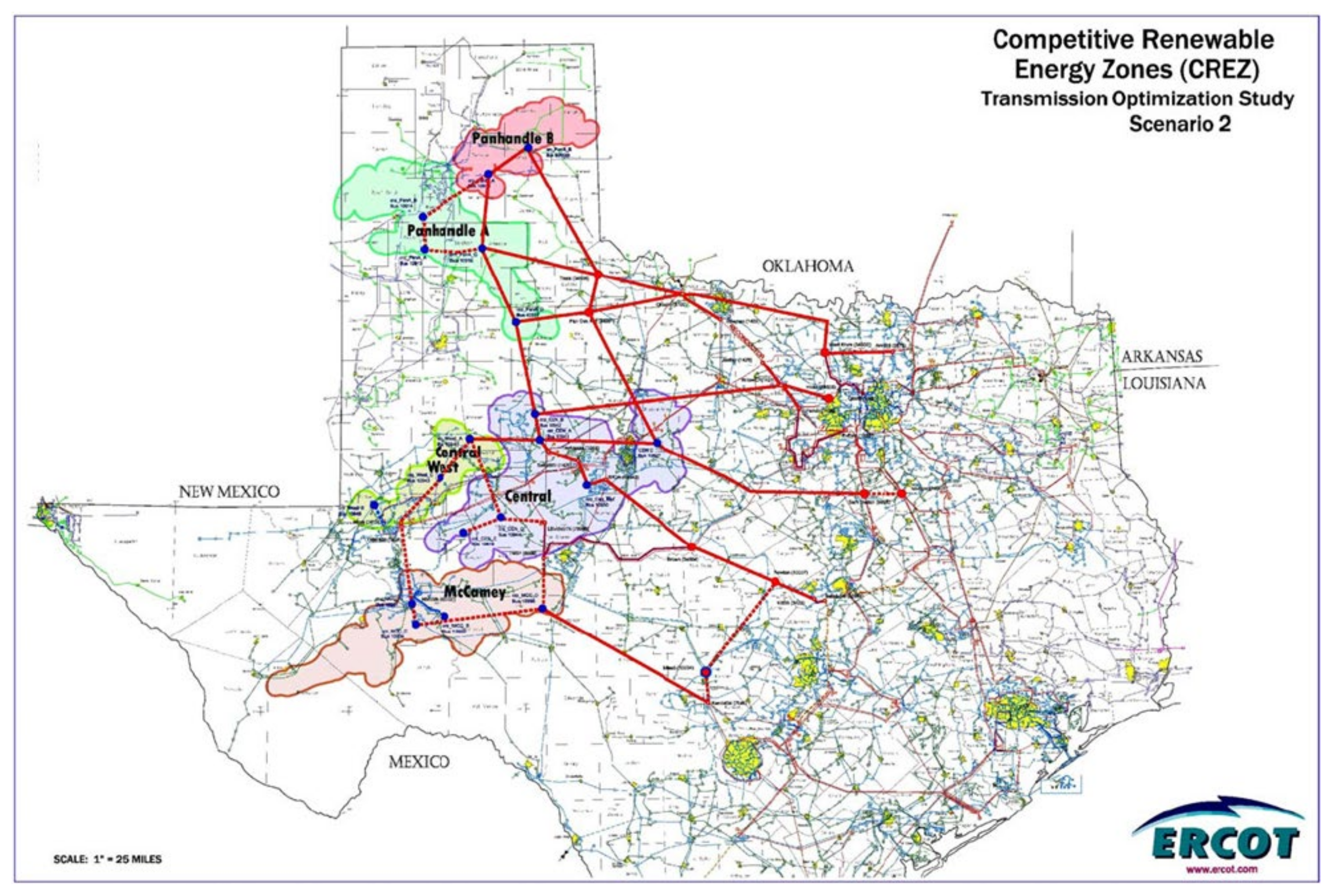
In the United States of America, similar to Germany, a scenario was created according to the capacity of renewable energy and a system reinforcement plan was established and system reinforcement was completed in 2014. In October 2007, the Public Utility Commission of Texas (PUCT or “commission”) issued an interim order which designated five areas as competitive renewable energy zones (CREZs) and requested that the Electric Reliability Council of Texas (ERCOT) and stakeholders develop transmission plans for four levels of wind capacity. The scenario configurations are shown in Table 3 below [10,11,12,13].
For example, the reinforcement plan for scenario 2 represents 3562 km for 345 kV right-of-way lines and 67.6 km for 138 kV right-of-way lines. The plan would provide adequate transmission capacity to accommodate a total of 18,456 MW for wind generation. The estimated cost of this plan is 4.93 billion US dollars. A diagram for CREZ scenario 2 is shown in Figure A1. In scenarios 3 and 4, reinforcement plans include HVDC. After constructing system reinforcement plans according to the given scenario, power system assessment and economic feasibility assessment were performed. Based on these results, the reinforcement of the transmission grid was completed on 30 January 2014, where 5800 km of 345 kV transmission lines were added with a total capacity of 18.5 GW. A diagram of the completed CREZ project is shown in Figure A2.
As the usage of renewable energy has increased, many have researched this topic and developed various techniques [14,15,16,17,18,19,20,21,22]. In order to maintain the reliability of power systems, research efforts have been directed at the development of two aspects, the first of which is assessing reliability based on voltage stability, angle stability, frequency stability and small-signal stability under the high penetration of inverter-based resources (IBRs). TSO was analyzed for a scenario with maximum power transfer from a renewable zone to a load center under various conditions, such as long-distance transfer, low inertia, high penetration of renewable energy, the dynamic characteristics of IBRs, new transmission lines, transient stability problems and reactive power control [14,15,16,17,18,19]. The second factor is investigating and carrying out grid expansion and the interconnection between grids and renewable zones when using HVDC. Projects associated with HVDC based on line-commutated converters (LCCs), voltage sourced converters (VSCs) and multi-terminal DC (MTDC) are actively progressing around the world and aim to expand renewable energy capacity and complement the disadvantages of transmission lines [20,21,22]. Various enhanced technologies for scenario development, IBR modeling, stability assessment and HVDC and so forth, have been applied and additionally researched in the context of power systems, including variable resources with high or medium penetration.
In this paper, optimal reinforcement measures for the accommodation of large-scale renewable energy are proposed. The methodology used in this paper is detailed below:
- First, a power system database (DB) containing a total of 63.8 GW of renewable energy is constructed. Scenarios with renewable energy capacities of 1 to 9 GW are established in the Sinan region.
- Second, renewable energy is modeled according to the Korean Grid Code standard. Renewable energy aggregation, reactive power supply capability, dynamic models and low-voltage ride-through (LVRT) standards are modeled in detail.
- Third, static and dynamic stability analyses are performed to examine the stability of renewable energy in connection with the power system considered here. Static analysis is performed for power flow analysis, contingency analysis, short-circuit analysis and robustness analysis. Dynamic analysis is performed for transient stability, frequency stability and LVRT analysis.
- Fourth, adequate grid reinforcement procedures are established according to the connection of renewable energy. After performing static and dynamic stability analyses for each scenario, grid reinforcement procedures based on transmission lines and HVDC are established. In selecting the grid reinforcement location, sensitivity analysis is performed and then reinforced at a substation with high sensitivity.
- Finally, after applying the reinforcement, some violations that cleared that the ESS and synchronous condenser were installed in the Shinan region.
2. Scenario Development
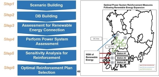
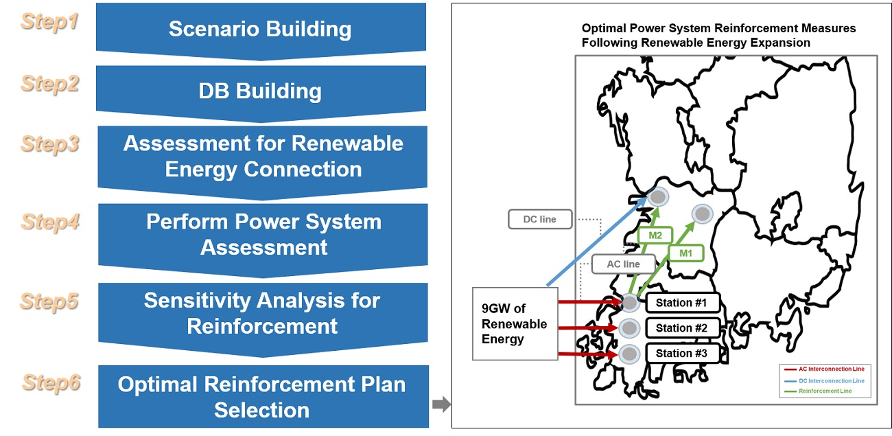
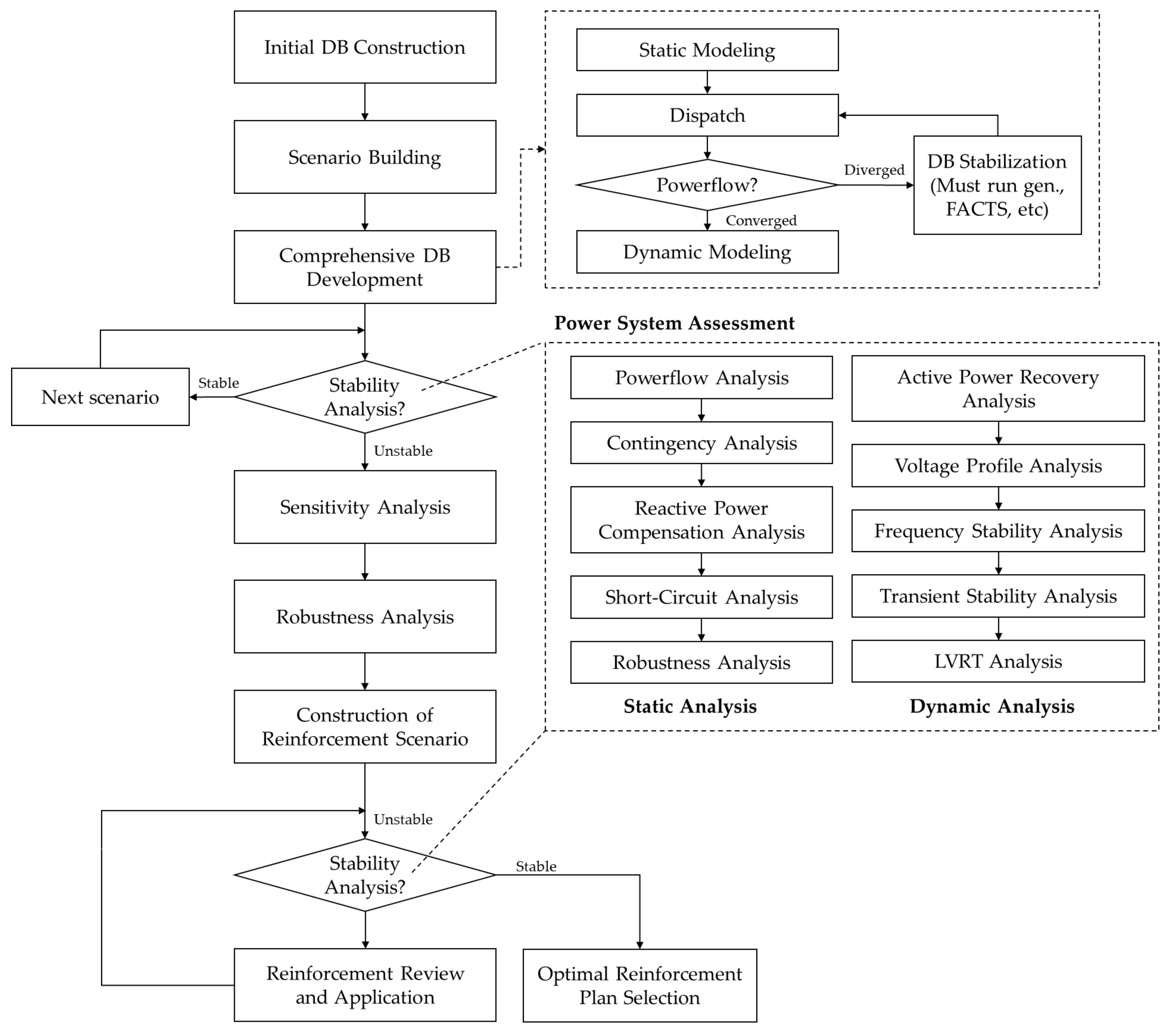
An overall flowchart of the reinforcement plan based on the study scenario is shown in Figure 2. Interconnection measures are designed to connect a large-scale renewable energy complex with an existing system and reinforcement measures are designed to strengthen an existing system to resolve system instability caused by renewable energy [23]. The major features are described as follows:
- An initial DB with the renewable energy capacity of 31.9 GW in 2026 and 63.8 GW in 2031 was created.
- Scenarios with renewable energy capacities of 1 to 9 GW were established in the Sinan region.
- A DB was built based on the convergence with respect to power flow calculation. The DB used in this paper was a Power System Simulator for Engineering (PSS/E)-based power system configuration database. As mentioned before, a total of 72 scenarios were constructed and analyzed using PSS/E. Each scenario consisted of power flow data and dynamic data. The power flow data were composed of bus, generator, load, transformer and transmission line data and so forth. Dynamic data were also considered, including the dynamic characteristic parameters of each piece of equipment. The power flow data and dynamic data related to a total of 72 scenarios were referred to as a PSS/E DB. The DB configuration in PSS/E is shown in Figure A3 and Figure A4.
- IBRs based on PV and wind type 3 and type 4 renewable generic models were applied.
- The interconnection measures of AC and HVDC lines were considered.
- After that, power system assessment was performed based on the DB configuring the interconnection measures. The method of configuring the interconnection measures in the DB was to create some buses at the interconnection point in the power flow data and to create the transmission line or HVDC line connecting the renewable energy complex and the interconnection bus. The interconnection measurement configuration in PSS/E is shown in Figure A5.
- In accordance with the stability results of the power system, the point of reinforcement was reviewed and applied, after which the power system was re-evaluated for the applied reinforcement measures.
The power system assessment was examined with both static analysis and dynamic analysis. The static analysis included overload, voltage violation, contingency, short-circuit capacity and reactive power compensation analyses. The dynamic analysis included active power recovery, voltage profile, frequency stability, transient stability and LVRT analyses. The steps used to generate the database for power system analysis were scenario building, generator modeling, dispatch, DB convergence and dynamic modeling.
2.1. Scenario Building
The renewable energy power system connection scenarios consist of:
- Separate scenarios for the years of 2026 and 2031.
- Demands of 60, 80 and 100% from a perspective of electricity supply and demand, where demand represents the scaled load for the maximum power consumption. If the load in 2030 is 100 GW, then 60% demand represents 60 GW.
- Constructing the initial DB and creating the scenario with renewable energy capacity between 1 and 9 GW.
- An AC line scenario and an AC and DC mixed scenario with approximately 7–9 GW of interconnection capacity.
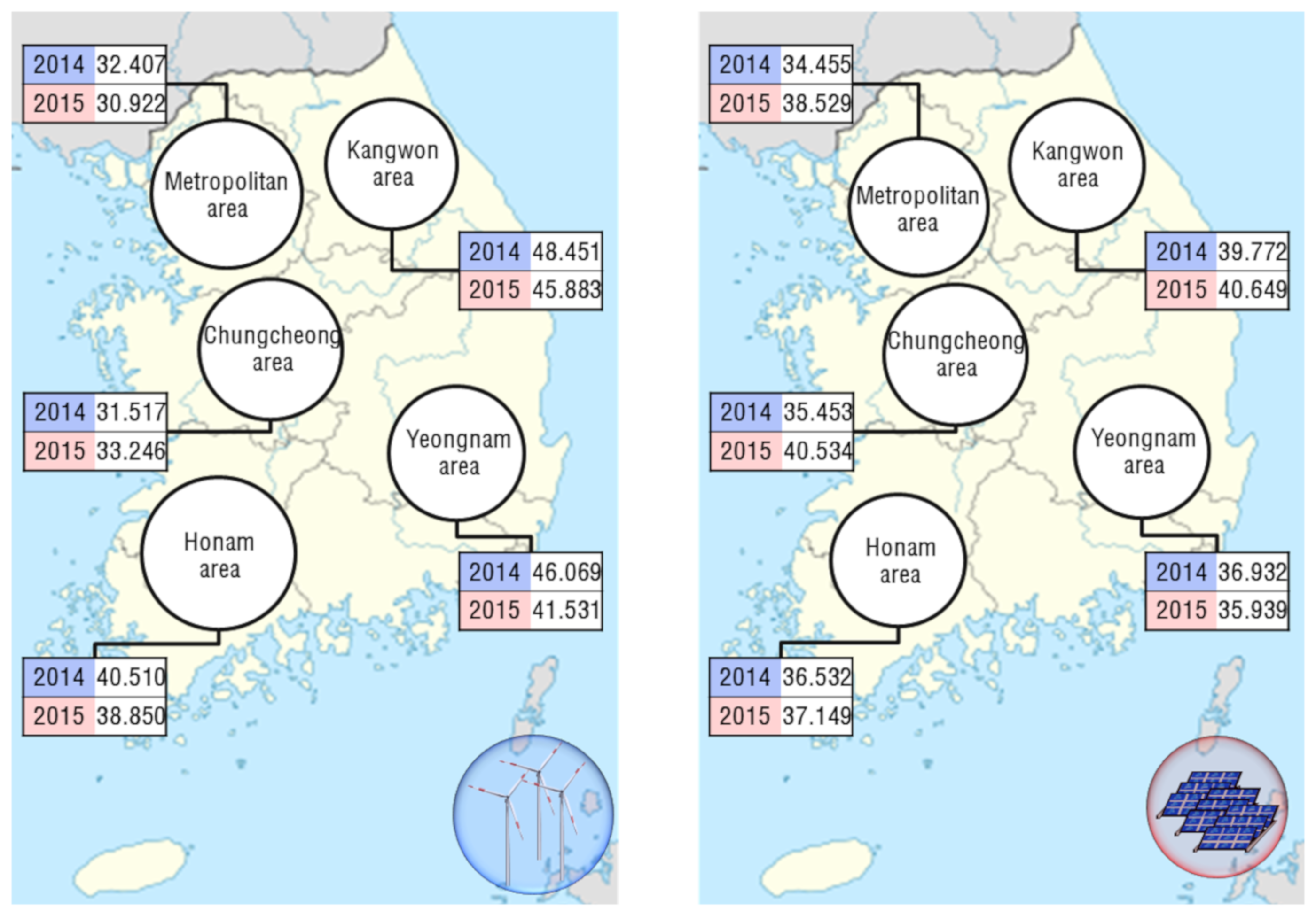
The scenarios were classified as shown in Table 4 through the above components. It is indicated when the renewable energy interconnection capacity is 1 GW at 100% demand, which is where scenario 1-1 applicable. Similarly, when the demand is 80%, the scenario is 2-1 and when the demand is 60%, the scenario is 3-1. In this way, scenarios were constructed for each 2026 and 2030. Scenario for demand of 60% represents only wind generation considering night. A total of 72 scenarios were constructed and analyzed. In this paper, the average capacity factor was used for all areas. Figure A6 and Figure A7 show the average and maximum values of the capacity factor in different areas for the years of 2014 and 2015. The capacity factor is defined as the ratio of actual power output over a period of time. In Korea, Korea Power Exchange (KPX), the power system operator, acquires and manages the amount of renewable energy output every hour. Considering the maximum capacity factor used in the 72 scenarios, the study of interconnection for installing 9 GW of renewable energy capacity is difficult to analyze because of convergence problems of power flow, voltage, transient instability and lack of inertia and so forth. Therefore, the average capacity factor was used for the renewable energy outputs in other areas and 9 GW of renewable energy was considered where the active power output of renewable energy is 100%.
2.2. DB Construction
2.2.1. Renewable Energy Modeling
In order to ensure the reliability of power system assessment for grid expansion, the methodology based on the Korean grid code for renewable energy was applied [24,25]. The standard for aggregation models was considered, that is, reactive power control and fault ride-through (FRT).
- (1)
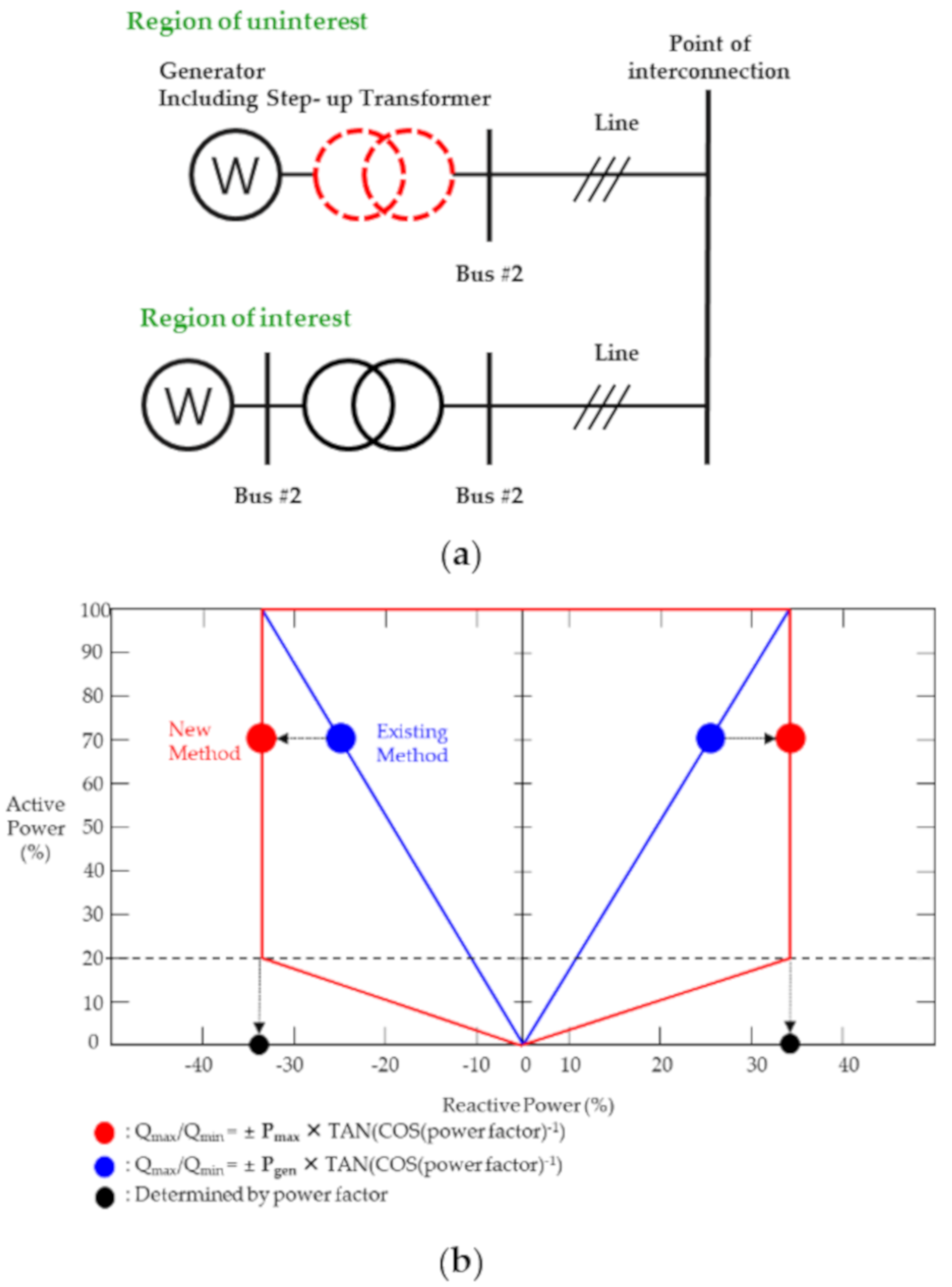
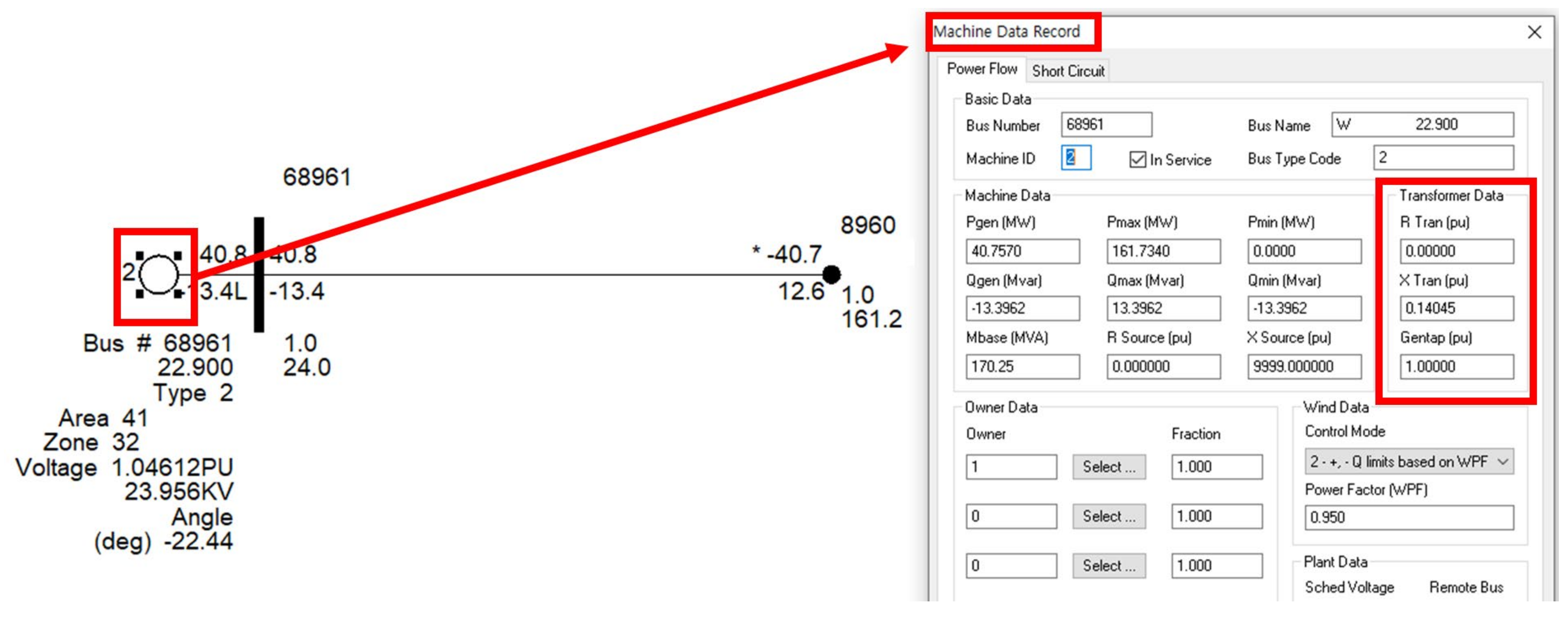
- Renewable energy generator modeling was conducted by classifying the region of interest and region of disinterest as shown in Figure 3a. For the region of disinterest, the modeling was conducted by an internal transformer via aggregation, while in the Sinan region the region of interest was modeled by constructing an external transformer. The internal transformer does not create a transformer between the bus and the generator in power flow data. In other words, the renewable energy was modeled as the generator including a step-up transformer (GSU). In PSS/E, the transformer data were included with the generator data [26]. The transformer configuration in PSS/E is shown in Figure A8 and Figure A9. The advantage of GSU could be decreased by the number of buses and equipment. In power flow analysis, renewable models between regions of interest and disinterest have small differences with respect to the reactive loss of transformers. In short-circuit analysis and dynamic simulation, the characteristics of two models with internal and external transformers are the same because the impedance of the internal transformer is included in numerical model. The size of the DB when using a renewable model based on an internal transformer is less than with an external transformer.
- (2)
- The reactive power capability for renewable energy was considered as shown in Figure 3b. It indicates the reactive power range according to the maximum output of renewable energy. In the existing method, the reactive power range depends on the actual renewable energy output. It is modeled by the renewable energy output and power factor. In the new method, the reactive power range depends on the maximum renewable energy output (i.e., the rated output). If the renewable energy output is less than 0.2 p.u., the reactive power range is reduced with the existing method. This means that the renewable energy based on a new grid code must be capable of supplying reactive power when outputting more than 0.2 p.u. of rated output [27]. The power factors of PV and wind power are 1.0 and 0.95, respectively. The control mode of PV power is composed of power factor control and wind power consists of a voltage control mode.
- (3)
- In FRT functions, LVRT is used to ensure a continuous voltage after failure.
Figure 3.
(a) Renewable energy model of disinterested and interested areas; (b) reactive power range according to the maximum active power and active power generation.
Figure 3.
(a) Renewable energy model of disinterested and interested areas; (b) reactive power range according to the maximum active power and active power generation.

2.2.2. Dynamic Modeling
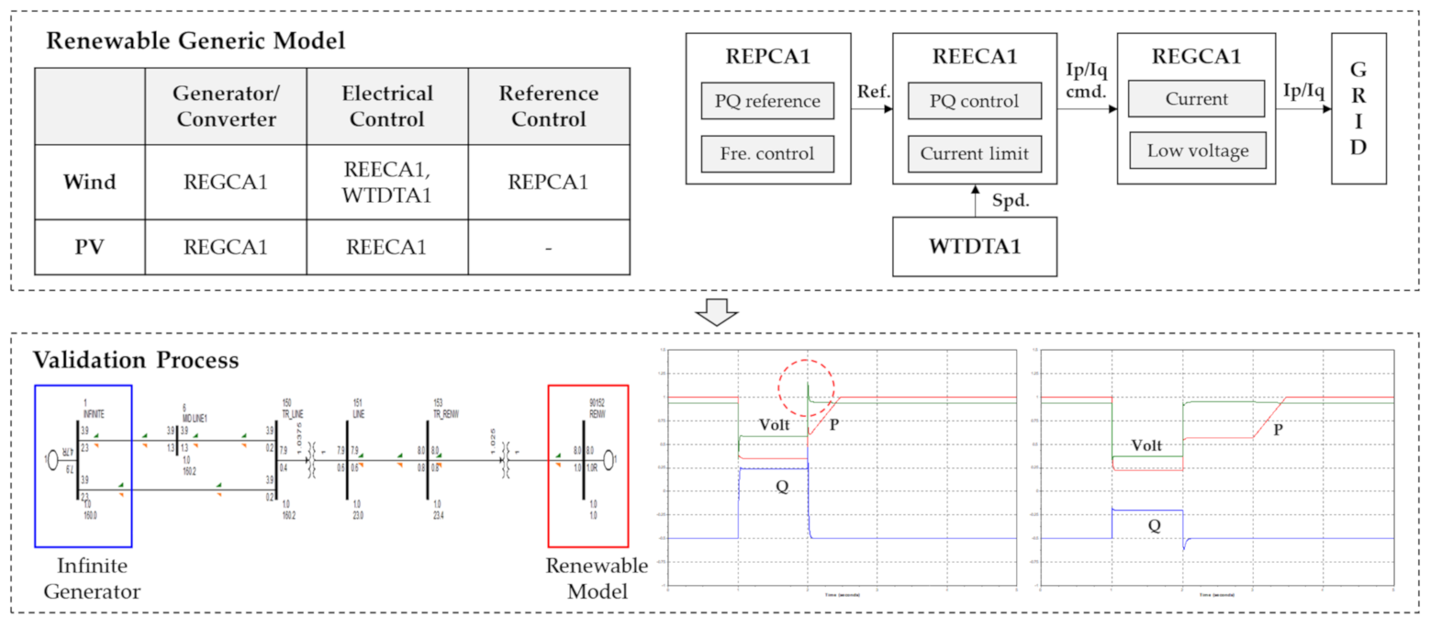
The dynamic modeling of IBRs that constitute large-scale renewable energy complex utilizes the generic model provided by PSS/E and the Western Electricity Coordinating Council (WECC) [26,28,29]. The generator model was created through REGCA1, along with the electrical model through REECA1, the mechanical turbine model through WTDTA1 and the reference control model through REPCA1. In the case of special installations, HVDC was composed of CDC4T, CDC7T and VSCDCT and the FACTS used CSTCNT. For the remaining special installations, the User Defined Model (UDM) dynamic model provided by the manufacturer was used. Figure 4 shows a dynamic model for a wind and PV system that was confirmed through validation. After the parameters with respect to the current limit, low voltage and control gain were tuned, the renewable generic model was applied for dynamic analysis.
3. Methodology for Connection and Reinforcement Plan
The configuration method for the interconnection line and data configuration, as well as the details for constructing optimal reinforcement measures, are described in the following sections.
3.1. Connection Measure
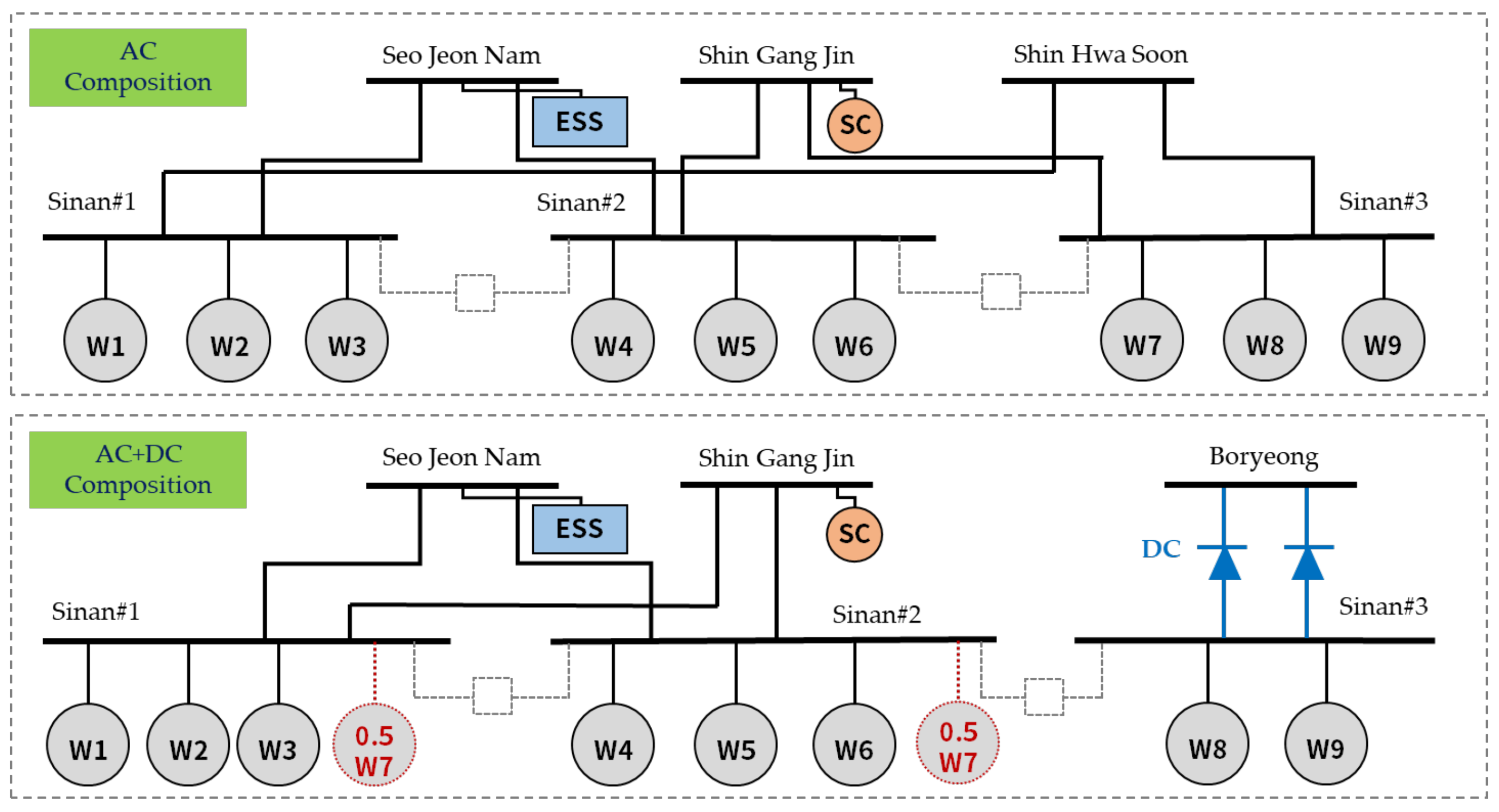
Two connection methods were used, where one method involved connection with AC lines only and another with AC and DC lines in combination. The interconnection line and busbar configuration can be seen in Figure 5.
All lines consisted of a double circuit transmission line. A DC interconnection line was added for only renewable energy capacities from 7 to 9 GW and not for all renewable energy capacities. The interconnection measure was composed of three stages using busbar separation. Specifically, when the renewable energy interconnection capacity was 1 to 3 GW, one AC line was used, while two AC lines were used for 4 to 6 GW and three AC lines or two AC lines and one DC line were used for 7 to 9 GW. The distance between Shin Hwa Soon station and Shinan #3 station is 30 km but the distance between Boryeong station and Shinan #3 station is 190 km. Because HVDC has benefits for transmitting bulk power over a long distance, a DC line was considered between Boryeong station and Shinan #3 station. For the line connecting the renewable energy complex to the land power system, the impedance of a submarine cable was applied. The detailed model data were applied to the 154 kV line of the Sinan region. For other cases, impedance with an 8 km line was applied. In the case of the capacity of the line, the AC line capacity was 3780 MVA and the DC line capacity was 1000 MW based on the 9 GW large-scale renewable energy complex.
3.2. Reinforcement
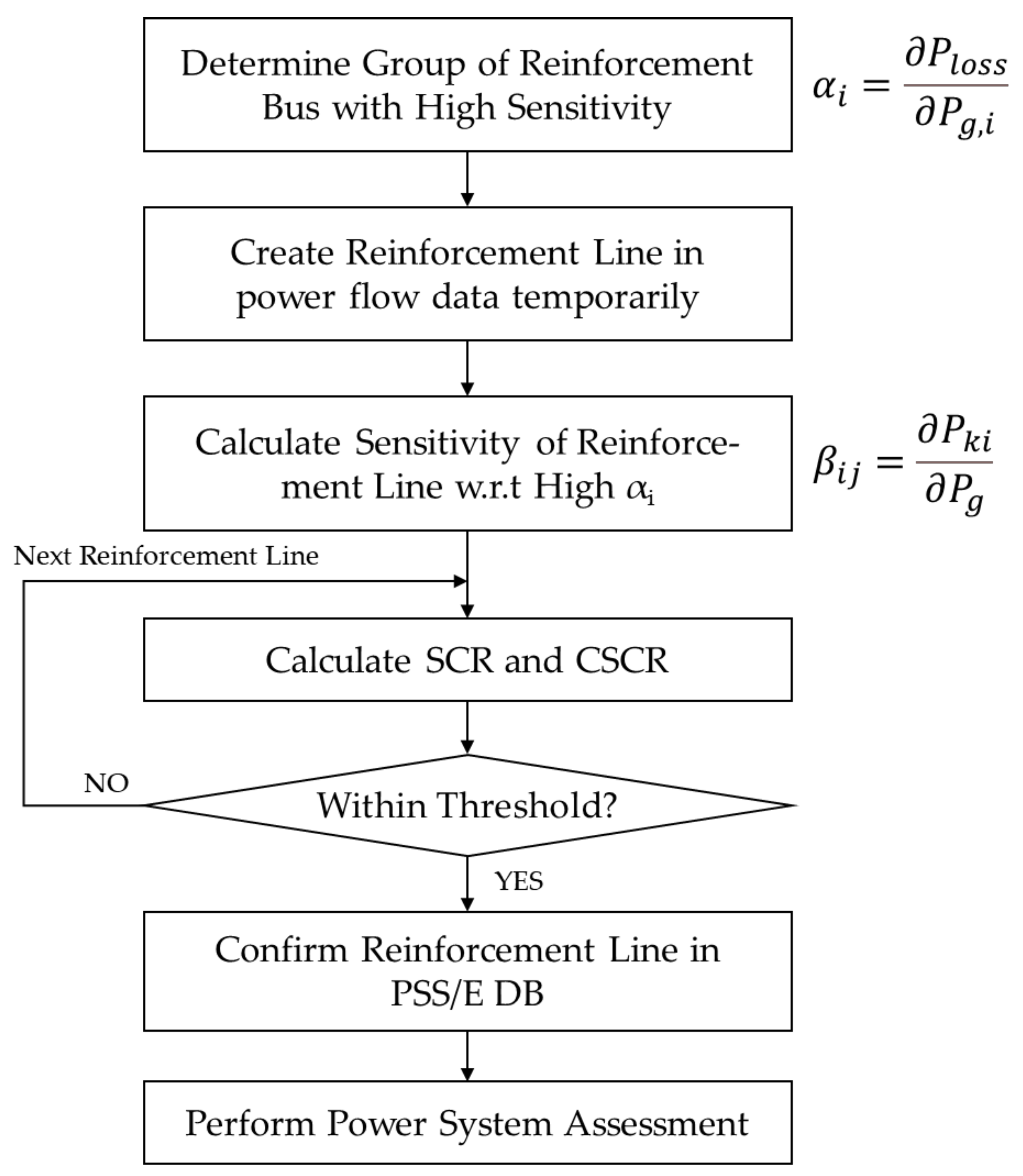
As shown in Figure 6, the reinforcement measure was established to solve the power system stability problems for when the power system weakens after linking renewable energy [17]. To determine the optimal reinforcement measure, a reinforcement proposal was first selected based on the sensitivity analysis. Afterward, the robustness analysis was carried out to decide whether the short-circuit ratio (SCR) and composite short-circuit ratio (CSCR) exceeded the threshold values. Then, the selected reinforcement measure was applied to conduct the power system assessment. The power system assessment is categorized into static and dynamic analyses, such as power flow analysis, contingency analysis, short-circuit analysis, transient stability analysis and frequency stability analysis and so forth. Lastly, the reinforcement measure was analyzed with the comprehensive results found by the static and dynamic analyses.
3.2.1. Sensitivity Analysis
Sensitivity analysis was used to measure the effect of an interconnection between a bus in an area with high renewable energy density and a remote bus in another area. The sensitivity analysis consisted of two steps [30]:
- Step 1: Analysis of the variation in transmission line loss following the injected power into the reinforcement bus. The sensitivity equation for the i-th bus can be compactly written as:where αi could be grouped for high sensitivity buses. With some power injected reinforcement buses, the buses with high sensitivity have a greater effect than buses with low sensitivity.
- Step 2: Analysis of the sensitivity between the reinforcement bus with high αi and renewable energy, representing the amount of change in a new reinforcement line per 1 MW increase in renewable energy. The sensitivity equation for the i-j line can be written as:where βij is calculated as the amount of change in the line after adding the reinforcement line. When a new reinforcement line is installed, a reinforcement plan with high sensitivity can cause more changes in a power system than a plan with low sensitivity.
3.2.2. Robustness Analysis
Robustness analysis was used to evaluate the performance of the power system as new renewable energy sources were connected. Three robustness analyses (short-circuit ratio (SCR), composite short-circuit ratio (CSCR) and weighted short-circuit ratio (WSCR)) were conducted and explanation of each is given as follows [11,31]: SCMVA denotes the short-circuit capacity before renewable energy connection and MWcap denotes the capacity of renewable energy.
- SCR: The robustness index for individual renewable energy connections. The typical standard is 2.0 or higher. Korea requires a value greater than 3.
- CSCR: The robustness index of a point of interconnection (POI) bus to which all renewable energy is connected. The international standard is 1.5 or higher. When the value is less than 1.7, reactive power compensation and grid reinforcement are required.
- WSCR: The robustness evaluation index of a region as defined by the Electric Reliability Council of Texas (ERCOT). The international standard is greater than 1.5. When the WSCR is less than 1.5, reactive power compensation and grid reinforcement are required; however, new domestic standards are needed for domestic applications. Due to the regional density of renewable energy sources, low values for the WSCR are typically calculated.
For the composition of the reinforcement measure, the compensated lines for the Yeongnam area and Honam area were investigated. Among the 10 reinforcement measures, 2 main types of compensated lines were identified. Additionally, due to the replacement of lines and transformers where constant overloads occur, a capacity increase of the current limiting reactor (CLR) of Uiryeong, in addition to the line type replacement for the Shin–Onyang–Chengyang and Shin–Gangjin–Gwangyang lines. Based on such measures, extreme overloads could be resolved. Hereinafter, the Gye-ryong reinforcement measure is referred to as reinforcement measure 1 and the Boryeong reinforcement measure is referred to as reinforcement measure 2. A configuration diagram of the reinforcement plans is presented in Figure 7.
4. Study Case
As explained above, the test systems were based on future Korean power systems for the years of 2026 and 2031. The system total generation values for the years of 2026 and 2031 were 92.1 and 99.0 GW, respectively. The number and capacities of HVDC systems connected to the metropolitan area were 3 and 12 GW, respectively. The case study includes static and dynamic analyses which were conducted with a DB excluding compensated lines according to the given scenario, followed by finding the time point for which reinforcement was needed. Afterward, a variety of reinforcement measures were added to the DB of a given scenario. Then, the optimal reinforcement measures were defined based on the review, as described in Figure 2.
4.1. Static Analysis before Reinforcement
For the static analysis, the weakness of the power system was analyzed based on the assessment of overload, voltage violation, contingency, short-circuit, reactive power requirement and robustness analyses.
4.1.1. Dispatch
Dispatch is when synchronous generators are stopped to maintain the balance of supply and demand as renewable energy generation increases. In this paper, because demand was fixed, the synchronous generators were adjusted according to the merit order. The merit order was based on an ascending order for the production price. Especially, when the generation of the considered metropolitan area was reduced, weak characteristics with respect to voltage stability and transient stability were present. Some generators must operate to maintain the robustness of the metropolitan area connected to the 765 kV transmission line and HVDC line. A reactive power compensation method such as a FACTS and/or switched shunting is then iteratively adjusted. New installations of FACTSs are considered to be minimal. The convergence of power flow analysis was secured to ensure the overall stability of the DB. After dispatch and DB stabilization, the power flow of the nationwide system became that shown in Figure 8.
4.1.2. Power Flow Analysis: Overload and Voltage Violation
Overloads occur when branch flows are different than the normal ratings for equipment. When the overload of lines and facilities becomes severe, it is difficult to transmit power. Table 5a shows the overload summary for various scenarios. Specifically, by year, overloads occurred when renewable energy was connected at 5 (2026) and 3 GW (2031). For both years, overloads occurred commonly at high connection capacities of 8 and 9 GW. This result is shown when the interconnection was conducted within measure 1, which connects large-scale renewable energy via only an AC line. When measure 2 was applied, which connects AC and DC together, the problem at 8 to 9 GW (which causes frequent overloads) was solved. Table 5 shows that the values for overloads were acceptable at 7 to 9 GW when a DC line was considered.
4.1.3. Power Flow Analysis: Voltage Violation
Based on the condition of voltage violation in Korea, voltage violation checks upon the connection of renewable energy lines are conducted [14,15,16]. Table 5b shows the number of voltage violations in the scenarios considered here. The number of voltage violations for a renewable energy capacity of 3 to 4 GW was more than that of 5 to 9 GW. From the connection of 5 GW, the convergence of the power flow analysis is wrong and voltage violations rapidly increased. This could be solved through the use of a small amount of reactive power compensation.
4.1.4. Contingency Analysis
In the contingency analysis, if the frequency of non-convergence increases then the power system cannot withstand various events, as well as further study, such as dynamic stability assessment (DSA). A typical way to solve non-convergence is by adding a transmission line and FATCS. Contingency analysis was performed for the contingency lists. The contingency lists consisted of 345 kV transmission lines in the Honam area, transmission lines between the Honam area and other areas and interconnection lines between a renewable energy capacity of 9 GW and the Honam area. In addition, the frequency of non-convergence cases, overloads and voltage violations were analyzed. As shown in Table 6, non-convergence cases were generated when the renewable energy connection capacity reached 5 GW in 2026. Similarly, a non-convergence case was created at 4 GW in 2031, causing the power system to weaken.
4.1.5. Short-Circuit Analysis
The fault current contribution of wind type 3 was usually 1.1 to 2.5 times the rated current. For wind type 4 and PV energy, the fault current contribution is 1.0 to 1.5 times the rated current [32]. As more renewable energy generators with 63.8 and 9 GW of capacity were added to the grid/Sinan region, it was confirmed that the number of short-circuit capacity violations increased, as shown in Table 7. To reduce the number of violations, busbar separation, new breaker installation and CLR installation should be considered. In this paper, it was considered that the number of existing CLRs at Uiryeong station should be increased. Notably, 345 kV transmission lines between Uiryeong station in the Yeongnam area and two stations in the Honam area have already been installed. In Korea, the threshold values for the short-circuit currents for the 345 kV bus and 154 kV bus are 63 kA and 50 kA, respectively. From a perspective of reinforcement measures, it was examined whether or not the threshold values were exceeded.
4.1.6. Reactive Power Compensation
A reactive power compensation (RPC) device was installed on the high-voltage side of the renewable energy transformer or the collector side. When applying interconnection measure 1, the reactive power compensation amount had the greatest deviation between the values when the renewable energy connection capacity was between 6 and 7 GW, as shown in Table 8.
Additional, as the renewable energy capacity increases, the amount of reactive power compensation increases significantly. As the amount of reactive power compensation increases, economical costs also increase. Therefore, it is important to achieve maximum efficiency with minimal compensation. When interconnection measure 2 was applied to resolve this problem, the reactive power was reduced significantly, thereby reducing the deviation between the reactive power at a 6 GW connection capacity and that at a 7 GW connection capacity, which leads to a reduced amount of reactive power compensation and a high renewable energy capacity.
4.1.7. Robustness Analysis
As mentioned before, the robustness analysis was carried out to decide whether the SCR and CSCR exceeded the threshold values. The threshold values of the SCR and CSCR are 2.0 and 1.5, respectively. Since the threshold value of the WSCR depends on the size of the region or renewable energy complex, only the patterns of fluctuation for the WSCR were analyzed.
Table 9 shows the robustness analysis results for the years of 2026 and 2031 and the minimum SCR and CSCR values were greater than the threshold values. As shown in Table 9, the minimum SCR has little variation in all scenarios and the CSCR and WSCR show the largest changes in the scenario with 4 GW. From the minimum values of the SCR, CSCSR and WSCR, the robustness of the grid began to decrease when a renewable energy capacity of 4 GW was connected.
4.2. Dynamic Analysis-before Reinforcement
The dynamic analysis results based on the active power recovery, voltage profile, frequency stability, transient stability and LVRT analyses were simulated for verification.
4.2.1. Active Power Recovery Analysis
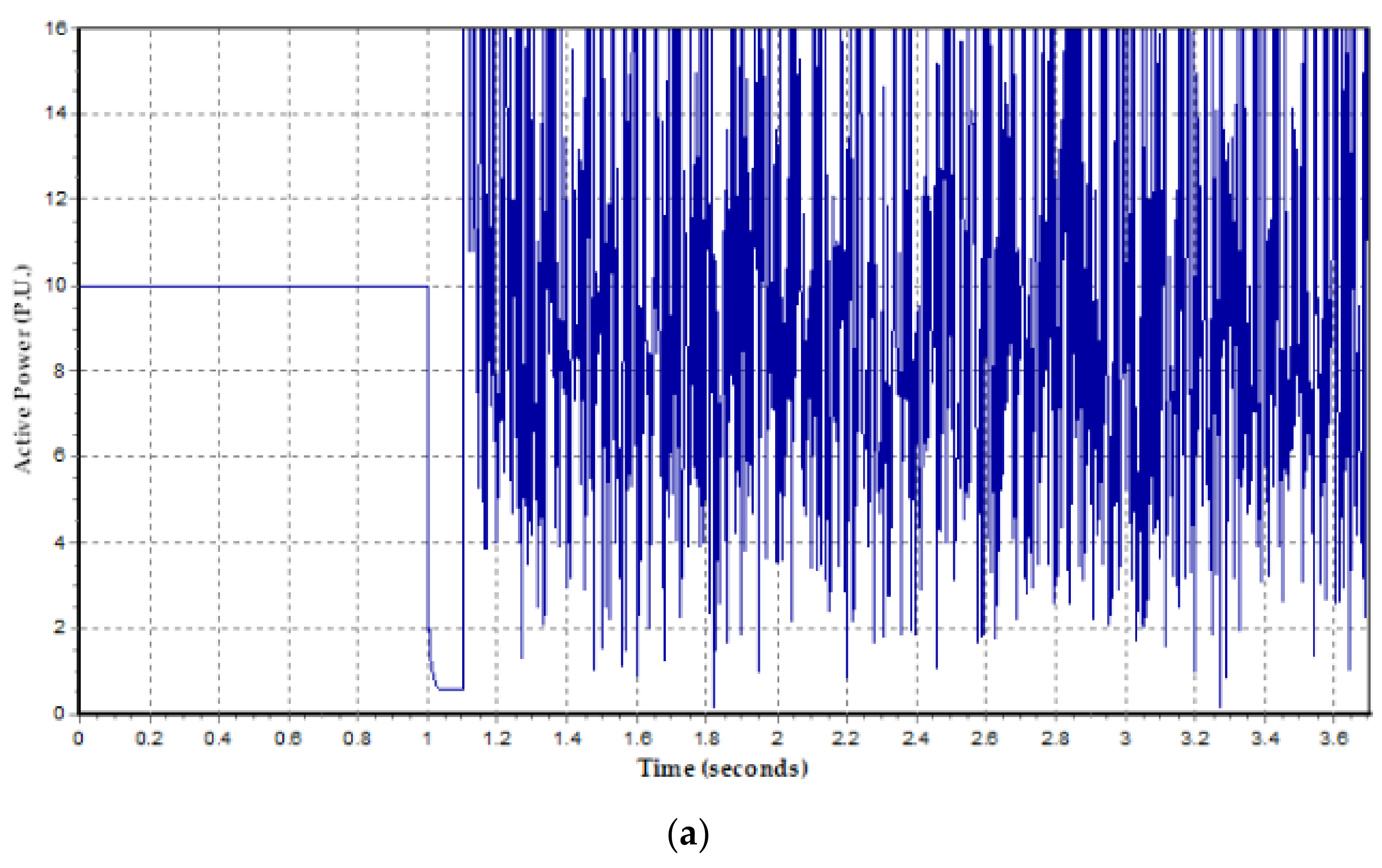
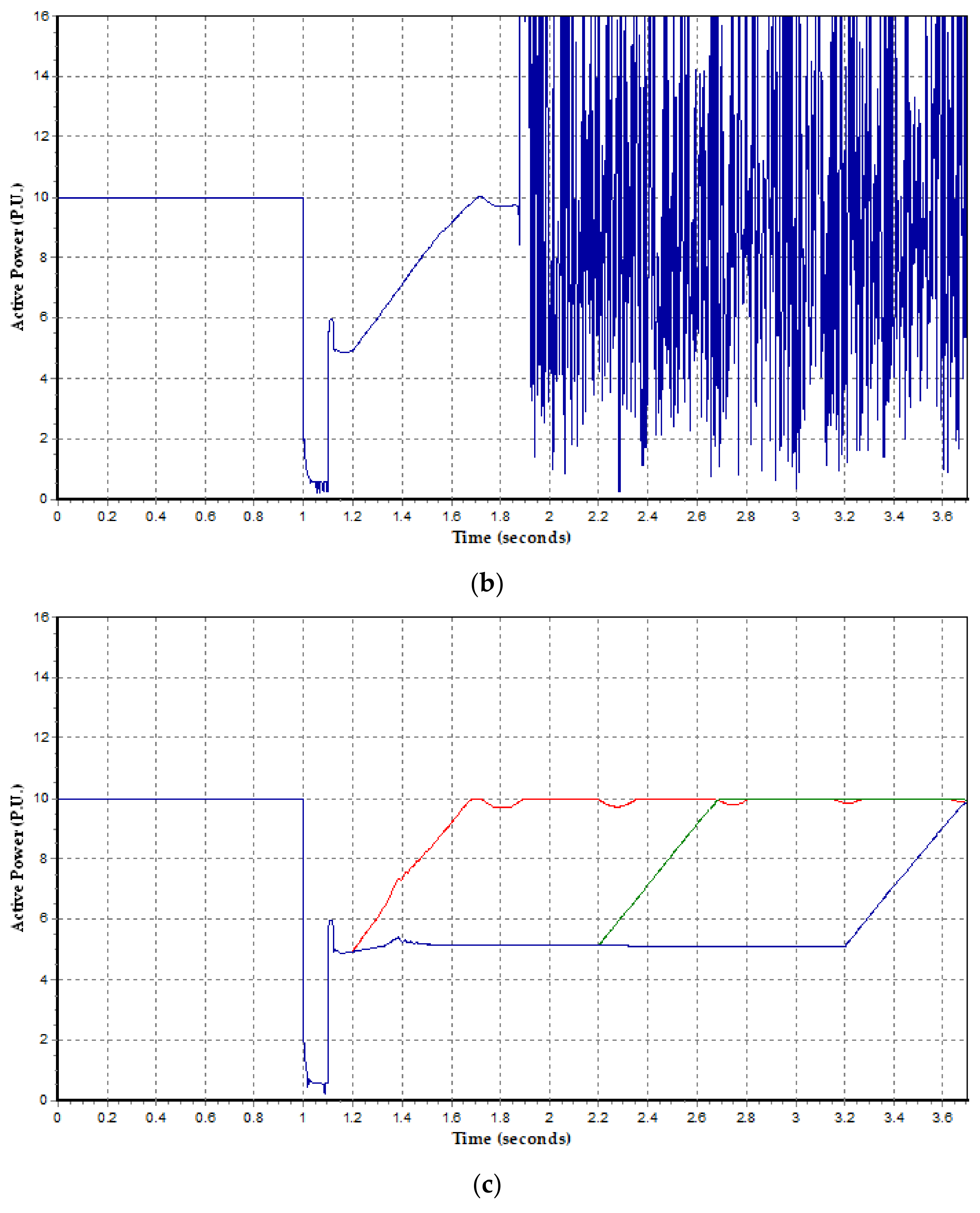
Active power recovery analysis was conducted to analyze the dynamic performance of renewable energy when a fault occurred at a concentrated area of large-scale renewable energy. The contingency was analyzed through a double circuit transmission line fault over the 345 kV line. As shown in Figure 9a, the problem of divergence occurs when the contingency is removed. To solve this problem, the parameters of dynamic simulation were changed. The acceleration factor was changed from 1.0 to 0.8, which determines the rate of change of the generation bus voltage per time step. Then, upon recovery of the active power, instability occurred due to simultaneous connection as shown in Figure 9b. Thus, the bus was separated and the parameters for the active power recovery time in REECA1 when interconnected at Shinan #1, Shinan #2 and Shinan #3 were set to 1.0, 2.0 and 3.0 s for sequential recovery. In addition, due to the instability on the 154 kV renewable energy connection bus, a FACTS with a small capacity was installed to maintain the characteristics of voltage after fault clearing. Figure 9c shows the active power after the bus spilt, parameter tuning and FACTS installation.
4.2.2. Voltage Profile Analysis
The purpose of voltage profile analysis is similar to active power recovery analysis, except for checking the voltage profile. In the voltage profile analysis here, the contingency lists consisted of the 345 kV transmission lines between Honam area and other areas and interconnection lines between a renewable energy capacity of 9 GW and the Honam area. The bus fault was introduced at 1 s and the fault elimination and line trip were introduced at 1.1 s, then finishing at 5.0 s. As shown in Table 10, in the 2026 case, non-converging cases were found at 8 GW. On the other hand, at 80 and 60% load demands in 2031, it can be seen that non-converging cases occur at 5 and 6 GW. It can be confirmed that better results could be derived by applying interconnection measure 2 for renewable energy connection capacities of 7 to 9 GW.
4.2.3. Frequency Stability Analysis
Frequency stability directly depends on the low inertia of synchronous generators when affected by an increase in renewable energy. Frequency stability analysis was conducted with a renewable generator drop of 1 GW and reserve power generation was set to 1.5 GW. In order to ensure the accuracy of the frequency stability analysis, the reserve power between static and dynamic reserves was identical when adjusting the parameters that governed the turbine. The static reserve denotes the reserve between the active power output of a unit (PGEN) and the maximum active power output of a unit (PMAX), while dynamic reserve denotes the reserve between the active power output of a unit and maximum power output of a turbine governor (PGOV). PGEN and PMAX were extracted from the power flow data in the PSS/E DB but PGOV was extracted from the dynamic data in the PSS/E DB. Static and dynamic reserves are typically defined as follows, where n is the total number of in-service units:
In Korea, the electrical frequency is between 60 and 59.7 Hz when dropping the 1 GW of generation capacity. This analysis proceeded by dropping the generator at 5 s then confirming the frequency response up until 60 s. As shown in Table 11, the frequency was stable at 100% load demand for all of 2026 and 2031, while most of the values fell out of the frequency stability range at a 4 GW connection capacity at 80 and 60% load demands.
4.2.4. Transient Stability Analysis
The transient stability was examined to evaluate the performance of the synchronous generators with respect to the rotor angle stability in the local area. The minimum critical clearing time for a three-phase fault is six cycles. The simulation conditions were identical to the voltage profile analysis. Based on these results, it was confirmed that the non-convergence of the rotor angle commonly occurred at 5 GW for both years of 2026 and 2031, as shown in Table 12. It can be confirmed that applying an interconnection measure 2 for a 5 GW renewable energy capacity yielded better results.
4.2.5. LVRT Analysis
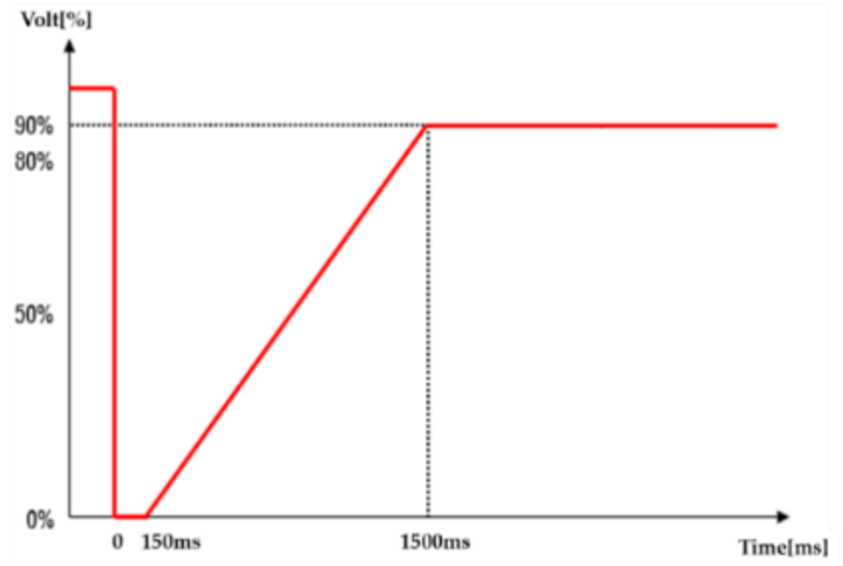
The LVRT analysis was conducted for buses of 154 kV or more in a nearby area connected to a large-scale renewable complex in order to confirm continuous voltage in the case of faults. The simulation conditions were identical to the transient stability analysis. The LVRT standard used is shown in Figure 10. As shown in Table 13, the results show that the connection capacity criteria were exceeded at 6 GW (100%), 4 GW (80%) and 5 (60%) according to the load demand for the year of 2026. For the year of 2031, the values commonly exceeded the LVRT at 5 GW.
4.3. Establishment of a Reinforcement Measure
The reinforcement measures were established based on the results of the static and dynamic analyses as shown in Table 14. From the results, reinforcement was necessary for the 5 GW connection in the years of 2026 and 2031. Although few violations for the LVRT and overload where found for the scenario with 4 GW, the violations could be resolved by installing small switched capacitors and increasing the capacity of one transmission line. In 2026, the problem of transient stability was not solved by the measures when applied to the scenario for 4 GW. For 2031, the overload, contingency analysis and transient stability could not be solved.
Sensitivity Analysis
The reinforcement measure in the Yeongnam region showed low values in the sensitivity analysis and was excluded from the reinforcement measure because no significant improvement was found in the analysis results. As shown in Table 15, only the results of the Gye-ryong reinforcement measure and Boryeong reinforcement measure were included, which show good values as a result of the reinforcement measures. The Gye-ryong reinforcement measure is referred to as reinforcement measure 1 here and the Boryeong reinforcement measure is referred to as reinforcement measure 2 here.
4.4. Static Analysis-After Reinforcement
Many of the issues of the power systems were improved by the reinforcement and the failure capacity increased slightly due to the addition of lines in some cases.
4.4.1. Power Flow Analysis: Overload and Voltage Violation
When reinforcement measures were applied as shown in Table 16, the overloads were then reduced or eliminated; however, in the case of the year of 2031, the overloads were not completely resolved at 8 and 9 GW upon reinforcement with reinforcement measure 1, whereas they were completely resolved by reinforcement measure 2. Based on the results, it can be confirmed that reinforcement measure 2 was more effective than reinforcement measure 1. In terms of the interconnection measures as well, when measure 2 was applied instead of measure 1, the overloads were eliminated completely. In terms of voltage violation, reinforcement measures 1 and 2 had similar results.
4.4.2. Contingency Analysis
In the contingency analysis, reinforcement measures 1 and 2 had similar non-convergence values in the 2026 case, as shown in Table 17. On the contrary, reinforcement measure 2 showed more stable values than reinforcement measure 1 in the 2031 case.
4.4.3. Short-Circuit Analysis
The reinforcement caused few changes in the short-circuit capacity, and, for reinforcement measures 1 and 2, there were similar short-circuit capacities, as shown in Table 18. For the station connected to many renewable farms in the Honam area, the capacity of the circuit breaker must be increased to withstand huge fault currents.
4.4.4. Reactive Power Compensation
Reactive power requirements varied with load demand for each renewable energy capacity; however, in most cases, the values were better for reinforcement measure 2 than reinforcement measure 1, as shown in Table 19. In addition, similarly, when interconnection measure 2 was applied, the reactive power requirement was less than with reinforcement measure 1.
4.5. Dynamic Analysis-after Reinforcement
Likewise, the dynamic analysis also showed improvements in many of the power system issues due to the reinforcement. Table 20 shows a summary of the dynamic analysis after reinforcement.
For the frequency stability analysis, when interconnection measure 2 was applied for the renewable energy connection capacity scenarios of 7 to 9 GW, the frequency increased slightly relative to that of interconnection measure 1. Nevertheless, it still fell outside the frequency stability range. Although no significant changes were observed in the frequency stability analysis as a result of the reinforcement measures, slight improvements were observed.
For the transient stability analysis, the values were the same for both reinforcement measures; however, in 2031, reinforcement measure 1 at 100%, reinforcement measure 2 at 80% and reinforcement measure 1 at 60% showed good values. When interconnection measure 2 was utilized, it generally converged and convergence was not attained for only the case of 9 GW with 80% load demand in 2031.
For the LVRT analysis, the addition of reinforcement measures resulted in improvements in cases of high interconnection capacity.
An example of the LVRT and transient stability analysis results is shown in Figure A10.
4.6. Additional Analysis
As additional analysis, after applying the reinforcement proposed in this paper, some violations for 80 and 60% demand occurred in dynamic analyses, such as in the transient stability and frequency stability analyses. To solve this problem, the installation of an ESS and synchronization condenser (SC) was additionally considered, as shown in Figure 5.
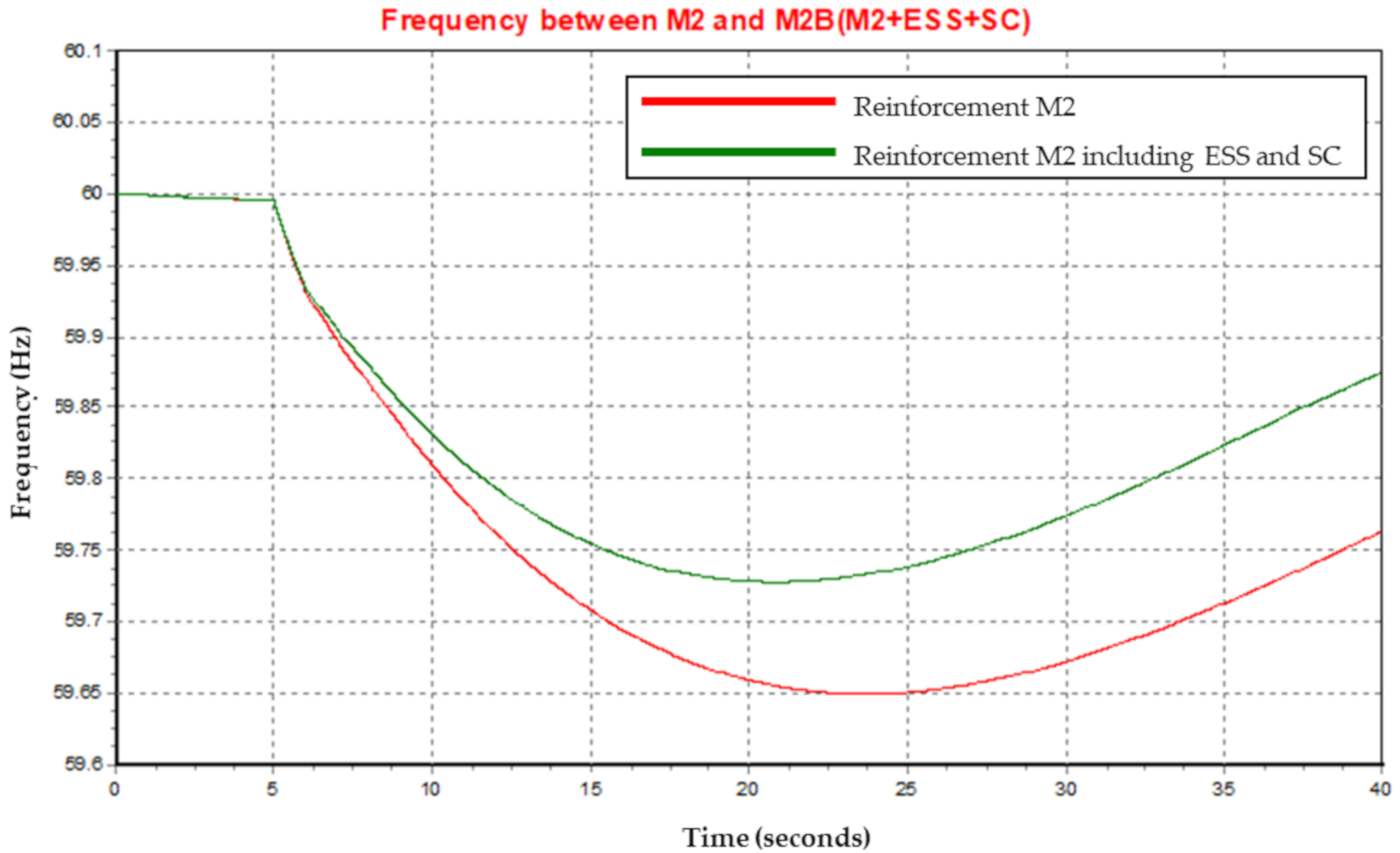
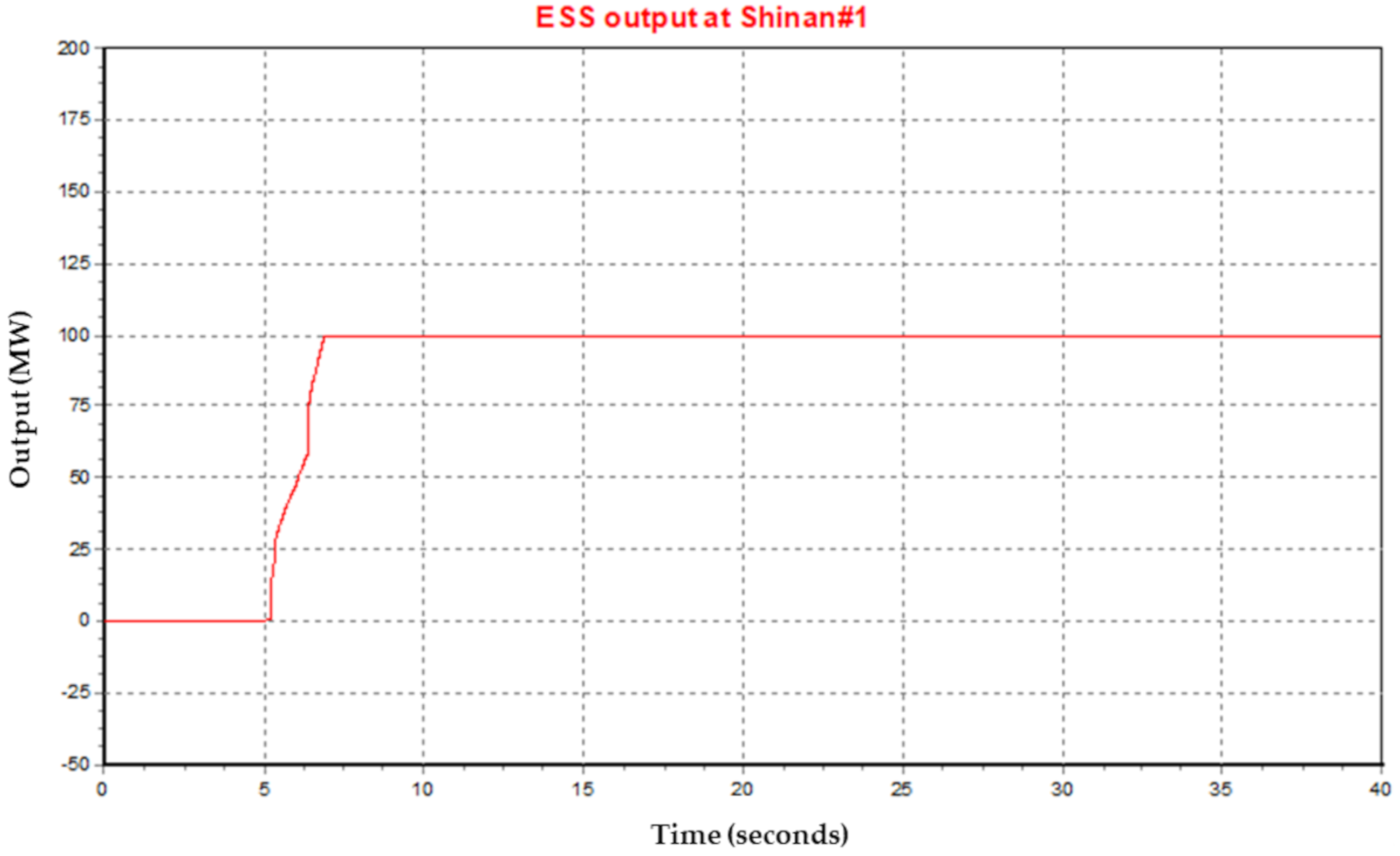
The additional dynamic analysis for reinforcement measure 2, including the ESS and SC, was performed at 80 and 60% demand in 2031. The simulation conditions were identical to the dynamic analysis without the ESS and SC. The capacities of the ESS and SC were 100 MVA each. Table 21 shows a summary of additional dynamic analysis for installing the ESS and SC. Reinforcement measure 2, including the ESS and SC at 80%, showed good performance as shown in Figure 11. The response of the ESS at contingency is shown in Figure 12. Reinforcement measure 2, including ESS and SC at 60%, showed good performance except for the results for the case of 9 GW in terms of the frequency stability and transient stability. If the capacities of the ESS and SC increased at 60% demand, all the violations that were found should not occur.
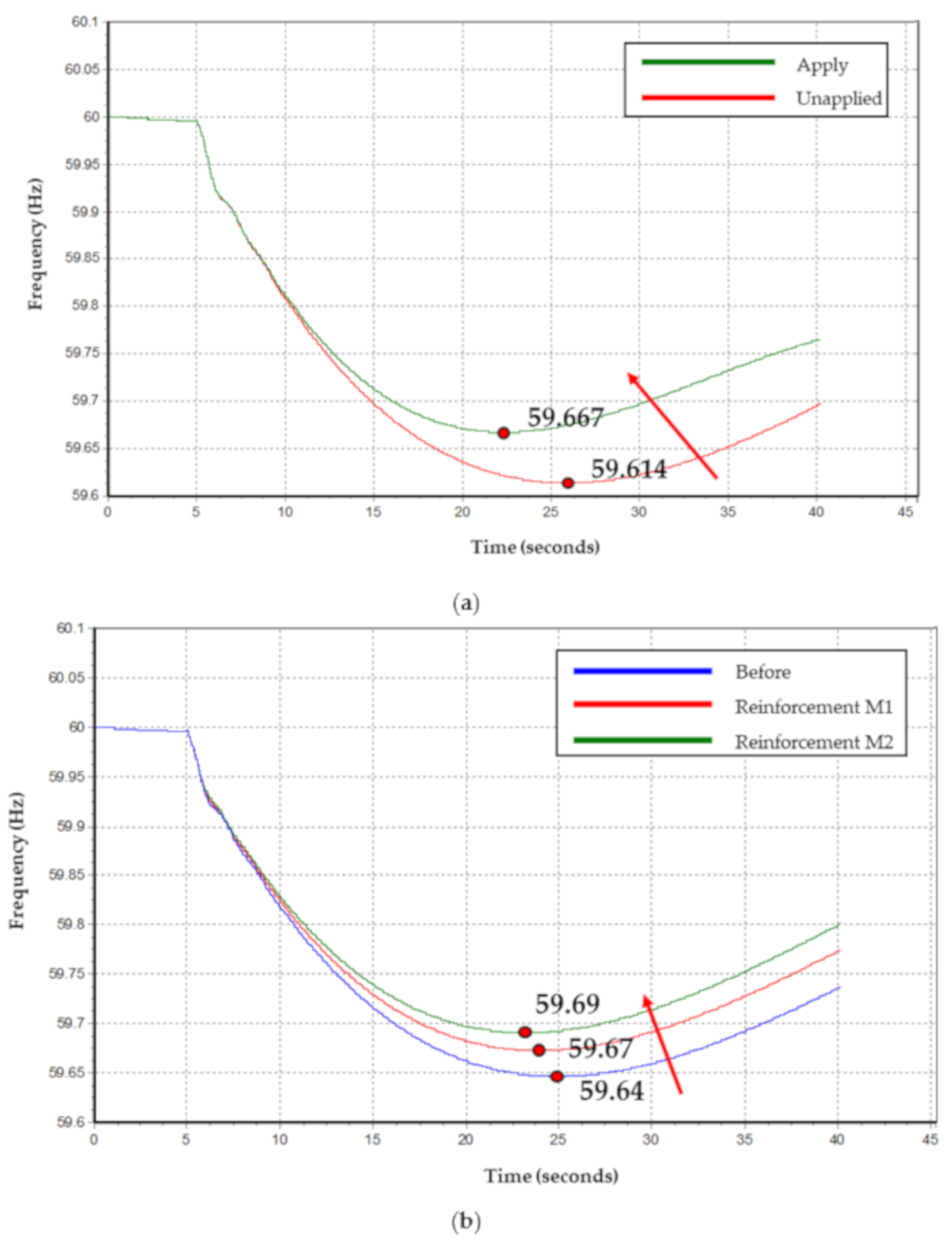
For the second additional analysis, note that when considering the reinforcement measures for applying or not applying the frequency response function of the wind turbine in the Sinan region that this results in the lowest frequency. As Figure 13 shows, it can be confirmed that the minimum frequency increased with the frequency response function and the line reinforcement of the wind power generator.
4.7. Summary
Table 22 shows the results of the comprehensive power system assessment for the years of 2026 and 2031 for a demand of 80%. In the four analyses of voltage violation, robustness, LVRT and active power recovery, the two reinforcement measures showed the same values. In the overload, contingency, short-circuit, frequency stability and transient stability analyses, reinforcement measure 2 showed better values. In the analysis of the voltage profile, reinforcement measure 1 showed a better value.
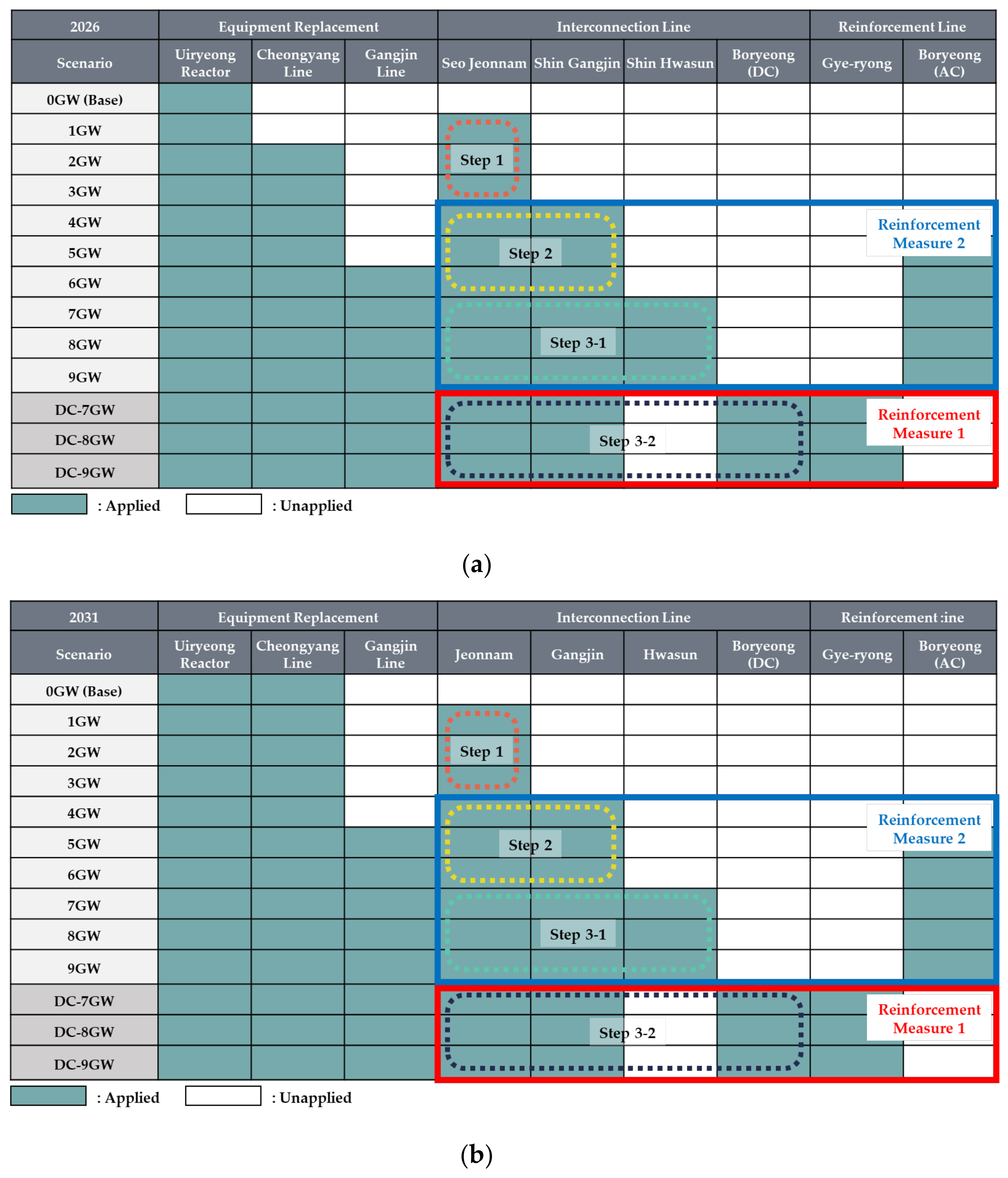
From the comprehensive results for the static and dynamic analyses based on the developed scenarios, the equipment reinforcement, interconnection line and reinforcement line were appropriately proposed by the optimal reinforcement measures. The power system stability was higher with interconnection measure 2 than under interconnection measure 1. If the connection capacity is less than 6 GW or only the AC line is used for connection, the Boryeong reinforcement measure is more conservative in terms of stability.
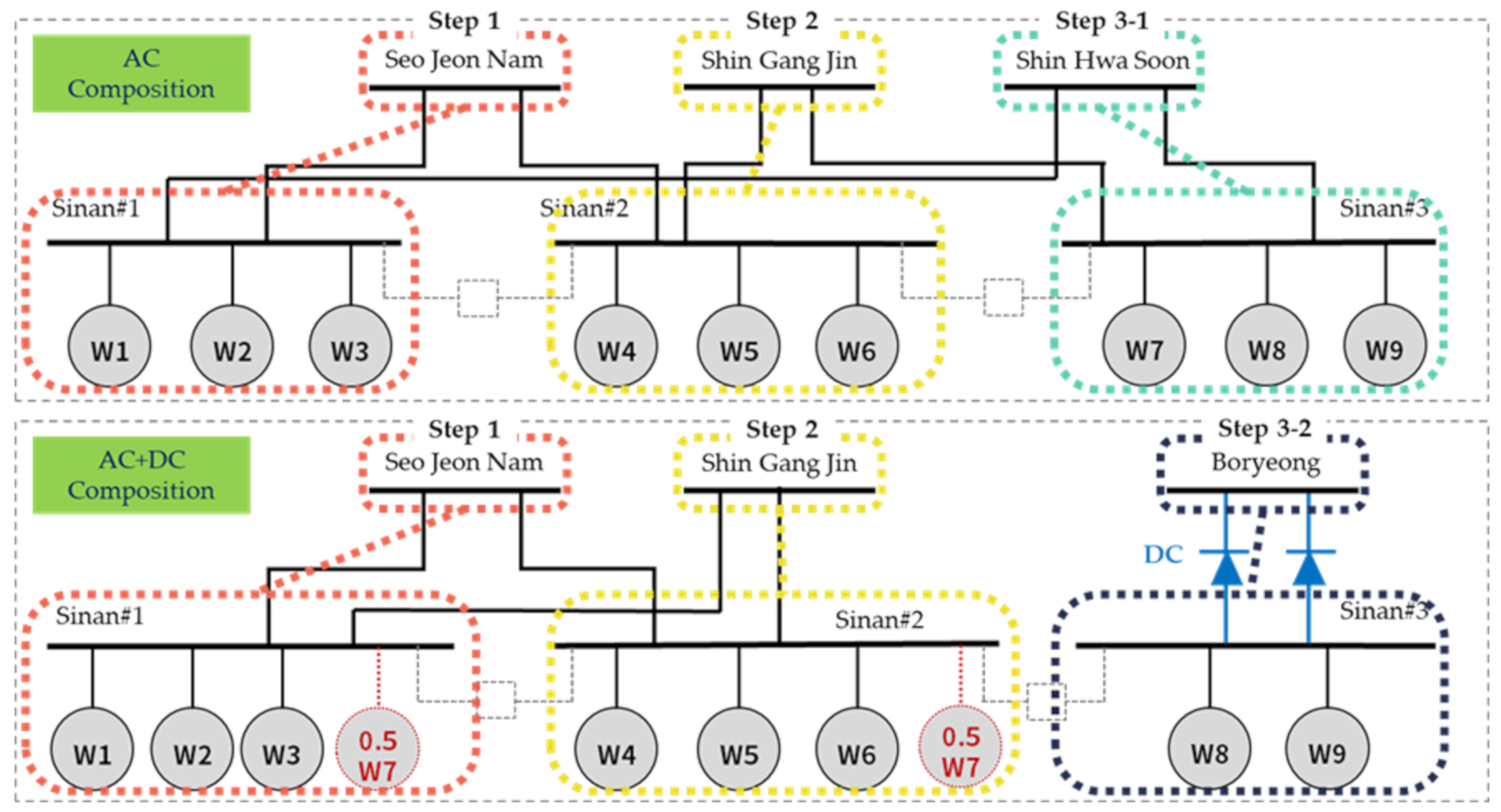
If a connection capacity is over 7 GW and the connection plan uses DC lines, then it is recommended to apply the Gye-ryong reinforcement measure proposed here. Reinforcement measure 2 has advantages due to the short distance and the topology and geographical factors of the Boryeong station with eight generators. Two generators will soon be retired there. There is a structural margin in the Boryeong station and power can be transmitted to the metropolitan area through the connected transmission line. Filling in a block means that an element has been applied and emptying the block means that an element has not been applied. Equipment replacement is to replace existing equipment as a solution to constant overloads. The interconnection line is a line for connecting renewable energy parks, as shown in Figure 14. The interconnection configuration was divided into three steps according to the capacity of renewable energy. Step 1 is approximately 1–3 GW, step 2 is approximately 4–6 GW and step 3 is approximately 7–9 GW. Step 3 is divided into AC configuration (Step 3-1) and AC + DC configuration (Step 3-1). The reinforcement measures were proposed by analyzing the effects of the interconnected and reinforced lines as shown in Figure 15.
5. Conclusions
In this paper, a methodology for reinforcing the power system in Korea has been proposed in order to solve the operational limitations and problems with the current power system due to the expansion of renewable energy sources. Based on the current status and plans for new and renewable energy at both home and abroad, a reinforcement plan was established and future power system scenarios were studied via connecting with a large-scale renewable energy complex. After an initial DB with a renewable energy capacity of 31.9 GW in 2026 and 63.8 GW in 2031 was created, 72 scenarios were established to assess the interconnection of renewable energy capacities varying between 1 and 9 GW in the Sinan region. Renewable energy scenarios based on an aggregated static model, IBR model and the LVRT standard were then developed. Then, the power system assessment was performed based on the scenarios, thereby configuring the interconnection measures, consisting of the AC line and HVDC.
The optimal reinforcement plan was derived as a result of the power system assessment. The results of the static and dynamic analyses indicate that the power system stability was higher under interconnection measure 2 than under interconnection measure 1. In addition, this paper recommends that reinforcement measures should be selected according to the connection capacity.
After applying the reinforcement proposed in this paper, some violations were found in the dynamic analyses, such as for the transient stability and frequency stability. In order to solve this, the installation of an ESS and synchronous condenser should be considered. In future research, the dynamic modeling of an ESS, the optimal placement of an ESS and synchronous condenser and operation strategies for ESSs will be considered.
Author Contributions
Project administration, S.-M.C.; Conceptualization, Y.-S.C.; Methodology, H.-I.K.; Formal analysis, H.-I.K.; Validation, Y.-S.C. and H.-I.K. All authors have read and agreed to the published version of the manuscript.
Funding
This research received no external funding.
Acknowledgments
This work was supported by “Human Resources Program in Energy Technology” of the Korea Institute of Energy Technology Evaluation and Planning (KETEP) and financial resources were granted by the Ministry of Trade, Industry & Energy, Korea (No. 20194010201760). This work was supported by the National Research Foundation of Korea (NRF) grant funded by the Korean government (MSIT) (No. NRF-2017R1D1A3B03035505).
Conflicts of Interest
The authors declare no conflict of interest.
Appendix A
The CREZ reinforcement plan for scenario 2 is shown in Figure A1. This plan contains 3562 km of 345 kV right-of-way and 67.6 km of 138 kV right-of-way. The plan would provide adequate transmission capacity to accommodate a total of 18,456 MW of wind generation. The estimated cost of this plan is 4.93 billion US dollars.
The CREZ reinforcement of the transmission grid was completed on 30 January 2014. The transmission network constructed 5800 km of 345 kV transmission lines with a total capacity of 18.5 GW. The cost of this plan was 6.9 billion US dollars. A CREZ reinforcement diagram is shown in Figure A2.
Figure A1.
CREZ reinforcement for scenario 2 [10].
Figure A1.
CREZ reinforcement for scenario 2 [10].

Figure A2.
Completed CREZ reinforcement [11].
Figure A2.
Completed CREZ reinforcement [11].

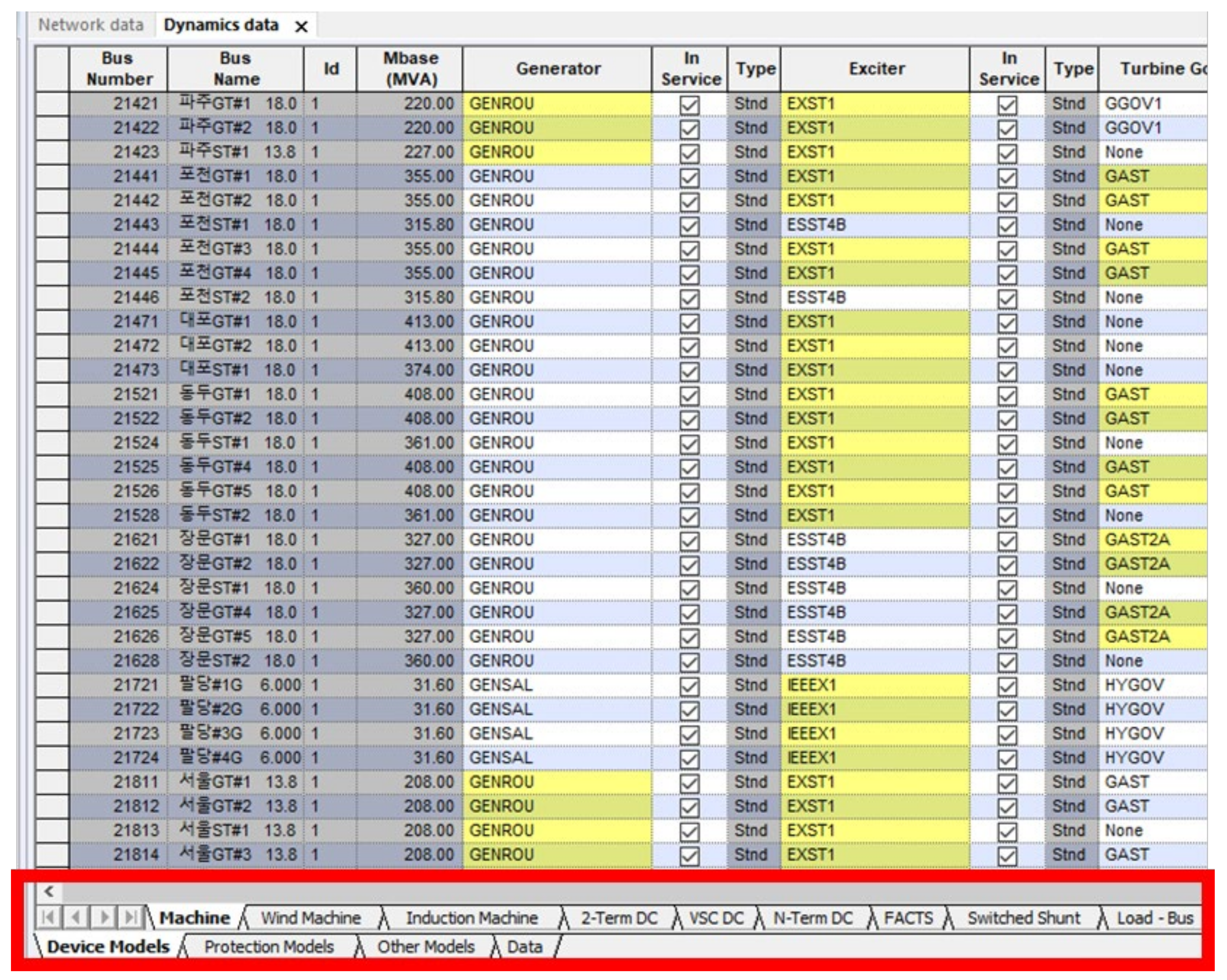
A total of 72 scenarios were constructed and analyzed using PSS/E. Each scenario consists of power flow data and dynamic data. The power flow data are composed of bus, generator, load, transformer and transmission line data and so forth. The power flow data are shown in Figure A3. There are also dynamic data, including the dynamic characteristic parameters of each equipment. The dynamic data are shown in Figure A4. The power flow data and dynamic data related to a total of 72 scenarios are referred to here as a PSS/E DB.
Figure A3.
Static DB based on PSS/E [26].
Figure A3.
Static DB based on PSS/E [26].

Figure A4.
Dynamic DB based on PSS/E [26].
Figure A4.
Dynamic DB based on PSS/E [26].

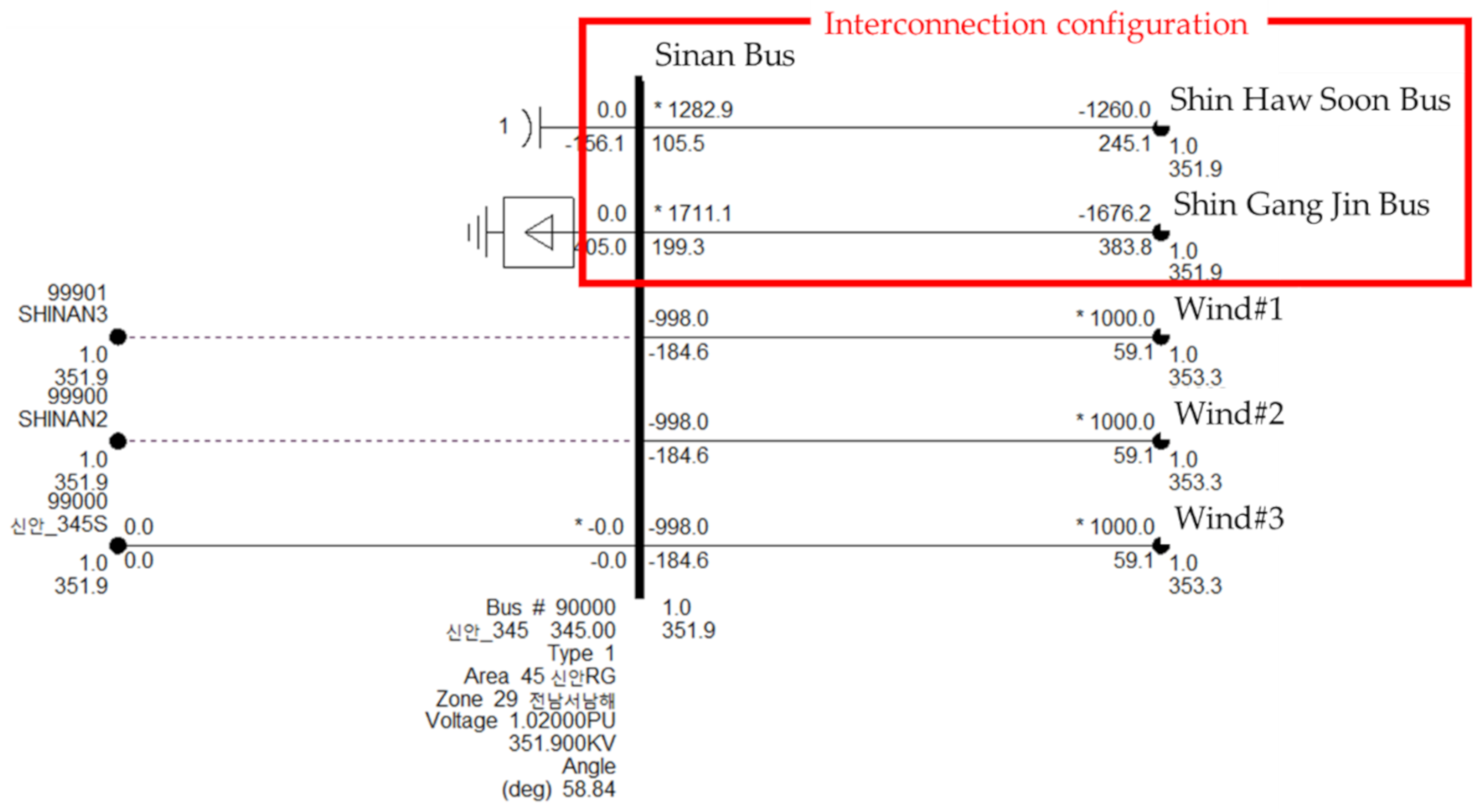
The meaning of “DB configuring the interconnection measures” is to create some buses at the interconnection point in the power flow data and to create a transmission line or HVDC line connecting the renewable energy complex and interconnection bus. The interconnection configuration is shown in the following Figure A5.
Figure A5.
Interconnection configuration on PSS/E [26].
Figure A5.
Interconnection configuration on PSS/E [26].

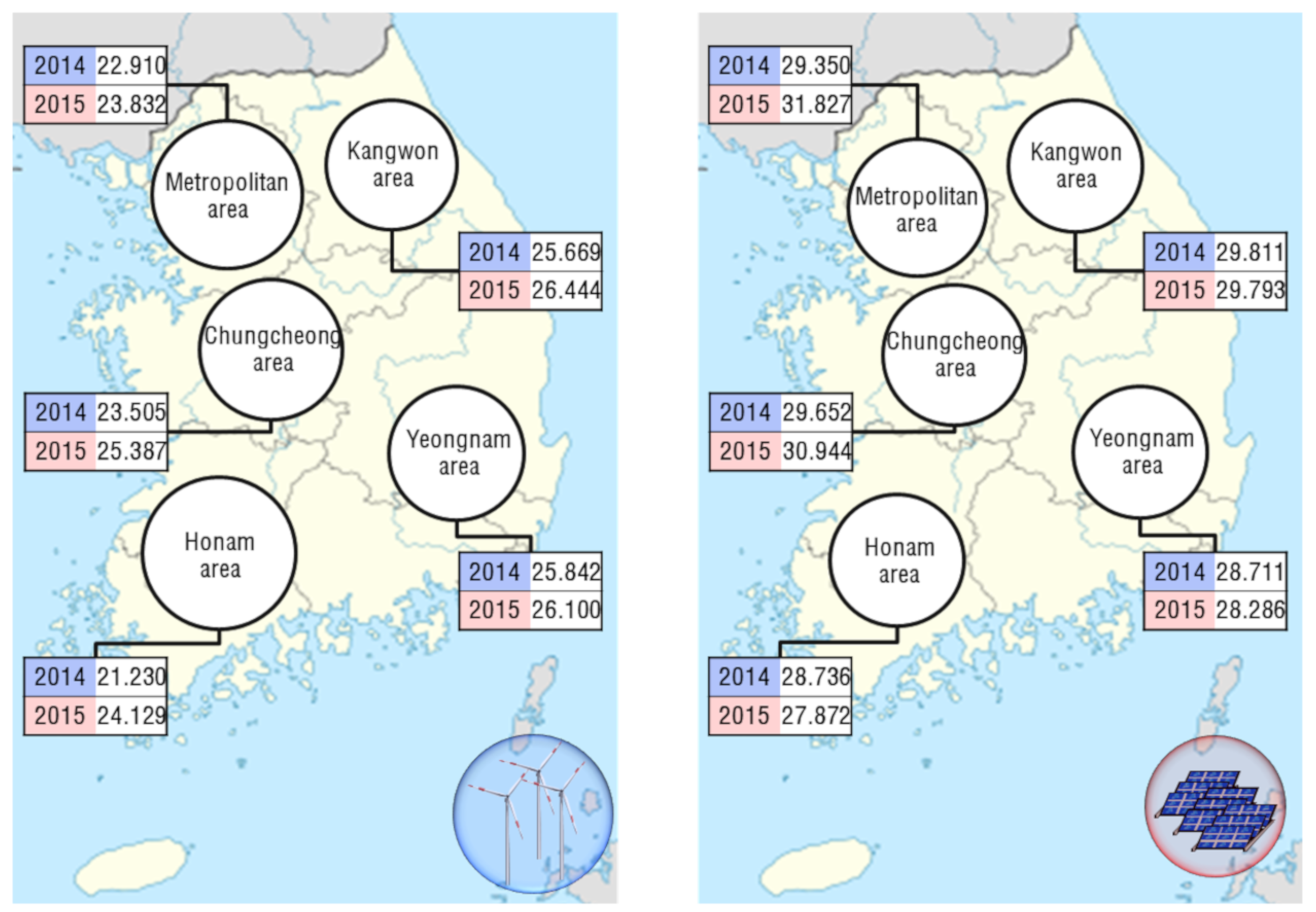
In this paper, the average capacity factor is used for all areas. Figure A6 and Figure A7 show the average and maximum values of the capacity factor in different areas for the years of 2014 and 2015. Capacity factor is defined as the ratio of actual power output over a period of time.
Figure A6.
Average capacity factor for renewable energy in different areas [33].
Figure A6.
Average capacity factor for renewable energy in different areas [33].

Figure A7.
Maximum capacity factor for renewable energy in different areas [33].
Figure A7.
Maximum capacity factor for renewable energy in different areas [33].

In this paper, the modeling of renewable energy is conducted by classifying regions of interest disinterest. The internal transformer does not create a transformer between the bus and the generator in power flow data. The internal transformer modeling based on PSS/E is shown in Figure A8. In other words, the renewable energy is modeled as the generator including the step-up transformer (GSU). The external transformer modeling based on PSS/E is shown in Figure A9.
Figure A8.
Internal transformer modeling based on PSS/E [26].
Figure A8.
Internal transformer modeling based on PSS/E [26].

Figure A9.
External transformer modeling based on PSS/E [26].
Figure A9.
External transformer modeling based on PSS/E [26].

Appendix B
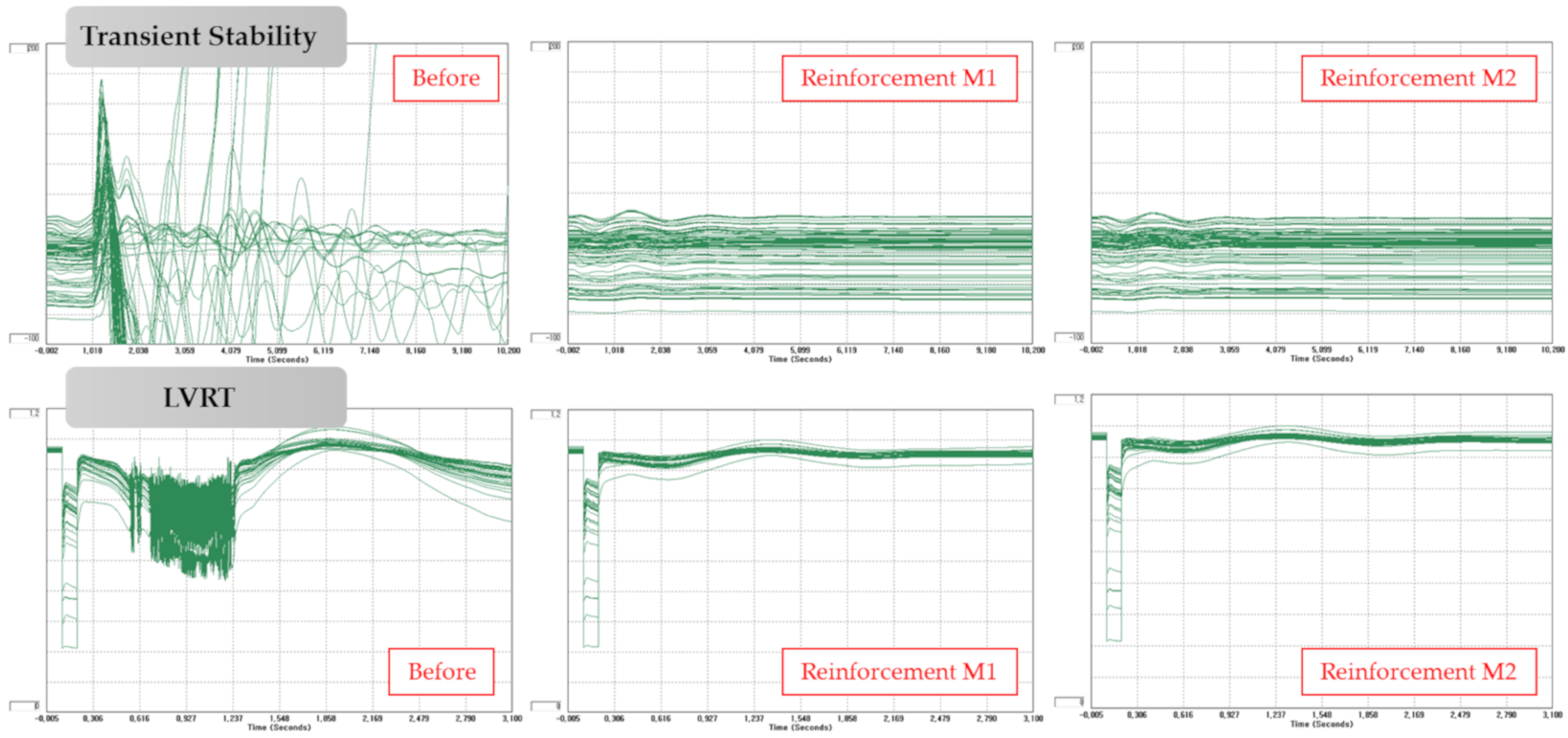
The power system assessment for deriving the optimal reinforcement plan is found here via the comparison of non-reinforcement (before), reinforcement M1 and reinforcement M2. Figure A10 shows the plots for the rotor angle in transient stability and voltage in the LVRT analysis.
Figure A10.
Plots for the rotor angle for the transient stability and voltage in the LVRT analysis according to the reinforcement measures.
Figure A10.
Plots for the rotor angle for the transient stability and voltage in the LVRT analysis according to the reinforcement measures.

References
- OECD. Trade in Embodied CO2 Database (TECO2). Available online: https://www.oecd.org/sti/ind/carbondioxideemissionsembodiedininternationaltrade.htm (accessed on 8 September 2020).
- Korea Power Exchange Supply and Demand Planning Team. Power Generation Station Capacity Change Document. Available online: http://epsis.kpx.or.kr/epsisnew/selectEkfaFclFepChart.do?menuId=020701 (accessed on 12 November 2020).
- KEPCO, Ministry of Trade, Industry, and Energy. Renewable Energy 3020 Implementation Plan. Available online: http://www.motie.go.kr/motie/ne/presse/press2/bbs/bbsView.do?bbs_cd_n=81&bbs_seq_n=159996 (accessed on 12 November 2020).
- KEPCO, Ministry of Trade, Industry, and Energy. 8th Basic Plan of Long-Term Electricity Supply and Demand. Available online: http://www.motie.go.kr/motie/ne/presse/press2/bbs/bbsView.do?bbs_cd_n=81&bbs_seq_n=160040 (accessed on 12 November 2020).
- Energiewende, A.; Ropenus, S.; Klinge Jacobsen, H. A Snapshot of the Danish Energy Transition: Objectives, Markets, Grid, Support Schemes and Acceptance. Study. Available online: https://orbit.dtu.dk/files/117987933/Agora_Snapshot_of_the_Danish_Energy_Transition_WEB.pdf (accessed on 12 November 2020).
- Energinet. Environmental report for Danish electricity and CHP for 2017 status year. Available online: https://en.energinet.dk/-/media/54B20C77CE954D7D98696520C23BAD6E.pdf (accessed on 12 November 2020).
- NETZ. NEUE NETZE FÜR NEUE ENERGIEN Der NEP 2012: Erläuterungen und Überblick der Ergebnisse. Available online: https://www.netzentwicklungsplan.de/sites/default/files/paragraphs-files/executive_summary_nep_2012_1_entwurf_neue_netze_fuer_neue_energien.pdf (accessed on 12 November 2020).
- Bundesministerium für Wirtschaft und Energie. Erneuerbare Energien in Zahlen Nationale und internationale Entwicklung im Jahr 2018. Available online: https://www.foerderdatenbank.de/FDB/Content/DE/Download/Publikation/Energie/erneuerbare-energien-in-zahlen-2018.pdf?__blob=publicationFile&v=2 (accessed on 12 November 2020).
- NETZ. Grid Development Plan 2030. Available online: https://www.netzentwicklungsplan.de/en/grid-development-plans/grid-development-plan-2030-2019 (accessed on 12 November 2020).
- ERCOT, System Planning. Competitive Renewable Energy Zones (CREZ) Transmission Optimization Study. Available online: https://www.nrc.gov/docs/ML0914/ML091420467.pdf (accessed on 12 November 2020).
- ERCOT; Lasher, W. The Competitive Renewable Energy Zones Process. Available online: https://www.energy.gov/sites/prod/files/2014/08/f18/c_lasher_qer_santafe_presentation.pdf (accessed on 12 November 2020).
- Lasher, W.P. The development of competitive Renewable Energy Zones in Texas. In Proceedings of the 2008 IEEE/PES Transmission and Distribution Conference and Exposition, Chicago, IL, USA, 21–24 April 2008; pp. 1–4. [Google Scholar]
- Schmall, J.; Huang, S.; Li, Y.; Billo, J.; Conto, J.; Zhang, Y. Voltage stability of large-scale wind plants integrated in weak networks: An ERCOT case study. In Proceedings of the 2015 IEEE Power & Energy Society General Meeting, Denver, CO, USA, 26–30 July 2015; pp. 1–5. [Google Scholar]
- Ehsan, R.; Megan, G.M.; John, S.; Shun, H.F.; Jeff, B. Stability Assessment of High Penetration of Inverter-Based Generation in the ERCOT Grid. In Proceedings of the IEEE Power Energy Society General Meeting, Atlanta, GA, USA, 4–8 August 2019; pp. 1–5. [Google Scholar]
- Edrah, M.; Lo, K.L.; Anaya-Lara, O. Impacts of High Penetration of DFIG Wind Turbines on Rotor Angle Stability of Power Systems. IEEE Trans. Sustain. Energy 2015, 6, 759–766. [Google Scholar] [CrossRef] [Green Version]
- Vittal, E.; O’Malley, M.; Keane, A. Rotor angle stability with high penetrations of wind generation. IEEE Trans. Power System 2012, 27, 353–362. [Google Scholar] [CrossRef]
- Mararakanye, N.; Bekker, B. Renewable energy integration impacts within the context of generator type, penetration level and grid characteristics. Renew. Sustain. Energy Rev. 2019, 108, 441–451. [Google Scholar] [CrossRef]
- Allard, S.; Mima, S.; Debusschere, V.; Quoc, T.T.; Criqui, P.; Hadjsaid, N. European Transmission Grid Expansion as a Flexibility Option in a Scenario of Large Scale Variable Renewable Energies Integration. Energy Econ. 2020, 87, 1–12. [Google Scholar] [CrossRef]
- Kumar, G.V.B.; Sarojini, R.K.; Palanisamy, K.; Padmanaban, S.; Holm-Nielsen, J.B. Large Scale Renewable Energy Integration: Issues and Solutions. Energies 2019, 12, 1996. [Google Scholar] [CrossRef] [Green Version]
- Alassi, A.; Banales, S.; Ellabban, O.; Adam, G.; Maclver, C. HVDC Transmission: Technology Review, Market Trends and Future. Renew. Sustain. Energy Rev. 2019, 112, 112–530. [Google Scholar] [CrossRef]
- Hofmann, F.; Schlott, M.; Kies, A.; Stocker, H. Flow Allocation in Meshed AC-DC Electricity Grids. Energies 2019, 13, 1233. [Google Scholar] [CrossRef] [Green Version]
- Pierri, E.; Binder, O.; Hemdan, N.G.; Kurrat, M. Challenge and Opportunities for a European HVDC grid. Renew. Sustain. Energy Rev. 2017, 70, 70–426. [Google Scholar] [CrossRef]
- Lee, N.; Flores-Espino, F.; Hurlbut, D. Renewable Energy Zone (REZ) Transmission Planning Process: A Guidebook for Practitioners; National Renewable Energy Laboratory: Golden, CO, USA, 2017. [Google Scholar]
- Korea Electric Power Corporation. Rules on the Use of Transmission and Distribution Facilities. Available online: http://cyber.kepco.co.kr/ckepco/front/jsp/CY/H/C/CYHCHP00601.jsp (accessed on 12 November 2020).
- Korea Power Exchange. Power System Market Operation Rules. Available online: https://www.kpx.or.kr/www/selectBbsNttView.do?key=29&bbsNo=114&nttNo=21499&searchCtgry=&searchCnd=all&searchKrwd=&pageIndex=1&integrDeptCode= (accessed on 12 November 2020).
- Siemens PTI, Documentation PSS/E 34 Operation, Application and Model Manual. Siemens: Munich, Germany, 2018.
- NREL. Review of PREPA Technical Requirements for Interconnecting Wind and Solar Generation; National Renewable Energy Lab (NREL): Golden, CO, USA, 2013. [Google Scholar]
- WECC. WECC Wind Plant Dynamic Modeling Guideline. Available online: https://www.wecc.org/reliability/wecc%20wind%20plant%20dynamic%20modeling%20guidelines.pdf (accessed on 12 November 2020).
- WECC. Solar Photovoltaic Power Plant Modeling and Validation Guideline. Available online: https://www.wecc.org/Reliability/Solar%20PV%20Plant%20Modeling%20and%20Validation%20Guidline.pdf (accessed on 12 November 2020).
- Wood, A.J.; Wollenberg, B.F.; Sheble, G.B. Power Generation, Operation, and Control; Wiley: Hoboken, NJ, USA, 2014. [Google Scholar]
- NERC. Integrating Inverter-Based Resources into Low Short Circuit Strength Systems Reliability Guideline. Available online: https://www.nerc.com/comm/PC_Reliability_Guidelines_DL/Item_4a._Integrating%20 _Inverter-Based_Resources_into_Low_Short_Circuit_Strength_Systems_-_2017-11-08-FINAL.pdf (accessed on 12 November 2020).
- IEEE Power System Relaying and Control Committee. Fault Current Contribution from Wind Plants; IEEE Power and Energy Society: Piscataway, NJ, USA, 2013. [Google Scholar]
- Hur, K.; Hur, J.; Cho, Y.S.; KEPCO. A Study on Power Grid Examination Standards of Renewable Energy and Policy of Public Network Reinforcement; Korea Electric Power Cooperation: Naju, Korea, 2017. [Google Scholar]
Figure 1.
The renewable energy “3020” implementation plan [3].
Figure 1.
The renewable energy “3020” implementation plan [3].

Figure 2.
The overall procedure for assessing the power system and establishing the reinforcement plan. FACTS: Flexible alternating current transmission system; DB: database; LVRT: low-voltage run-through.
Figure 2.
The overall procedure for assessing the power system and establishing the reinforcement plan. FACTS: Flexible alternating current transmission system; DB: database; LVRT: low-voltage run-through.

Figure 4.
Dynamic model of renewable energy.

Figure 5.
System diagram according to interconnection measures and interconnection capacity.

Figure 6.
The process to find the optimal placement of the reinforcement plan.

Figure 7.
System diagram according to interconnection lines and reinforcement lines.

Figure 8.
Power flow system diagram before and after dispatch due to renewable energy interconnection.
Figure 8.
Power flow system diagram before and after dispatch due to renewable energy interconnection.

Figure 9.
(a) Non-convergence problem after fault removal; (b) recovery of the active power via adjusting simulation parameters; (c) active power recovery through dynamic parameter tuning.
Figure 9.
(a) Non-convergence problem after fault removal; (b) recovery of the active power via adjusting simulation parameters; (c) active power recovery through dynamic parameter tuning.


Figure 10.
Low-voltage ride-through (LVRT) standard in Korea.

Figure 11.
Frequency between M2 and M2B.

Figure 12.
ESS output at Shinan #1.

Figure 13.
(a) Frequency response in the year of 2026 according to the application and non-application of a frequency response function for the wind generator in the Sinan region; (b) lowest frequency change according to the base status (before), reinforcement 1 and reinforcement 2 in the year of 2026.

Figure 14.
System diagram according to the connection steps.

Figure 15.
(a) Reinforcing elements according to the interconnection capacity in 2026; (b) reinforcing elements according to the interconnection capacity in 2031.
Figure 15.
(a) Reinforcing elements according to the interconnection capacity in 2026; (b) reinforcing elements according to the interconnection capacity in 2031.


Table 1.
Predicted renewable energy generation capacity of 2030 by region (GW).
| Source | Metropolitan | Gangwon | Chungcheong | Honam | Yeongnam | Jeju |
|---|---|---|---|---|---|---|
| Photovoltaic | 4.5 | 2.7 | 6.3 | 13.0 | 6.6 | 0.5 |
| Wind | 0.7 | 3.9 | 0.9 | 5.4 | 6.3 | 0.5 |
| Other | 1.7 | 0.5 | 1.8 | 1.8 | 1.5 | - |
| Total | 6.9 | 7.1 | 9.0 | 20.2 | 14.4 | 1.0 |
Table 2.
Periodic countermeasures against wind power volatility defined by Denmark’s transmission system operator (TSO) [5].
Table 2.
Periodic countermeasures against wind power volatility defined by Denmark’s transmission system operator (TSO) [5].
| 2020 | 2035 | 2050 | |
|---|---|---|---|
| General goals | Reduction in greenhouse gas emissions by 40% | Independence from fossil fuels in all sectors | |
| Renewable energy sources | 35% share of renewable energy sources in total | 100% renewable share as a cross-sectoral target | |
| Electricity sector | 50% wind share in electricity consumption | 100% renewables in the electricity sector | 100% renewable share as a cross-sectoral target |
Table 3.
MW tiers proposed by the Electric Reliability Council of Texas (ERCOT) for competitive renewable energy zones (CREZs) in a transmission optimization study [10].
Table 3.
MW tiers proposed by the Electric Reliability Council of Texas (ERCOT) for competitive renewable energy zones (CREZs) in a transmission optimization study [10].
| Scenario 1 (MW) | Scenario 2 (MW) | Scenario 3 (MW) | Scenario 4 (MW) | |
|---|---|---|---|---|
| Panhandle A | 1422 | 3191 | 4960 | 6660 |
| Panhandle B | 1067 | 2393 | 3270 | 0 |
| McCamey | 829 | 1859 | 2890 | 3190 |
| Central | 1358 | 3047 | 4735 | 5615 |
| Central West | 474 | 1063 | 1651 | 2051 |
| CREZ Wind | 5150 | 11,553 | 17,956 | 17,516 |
Table 4.
Scenario for renewable energy interconnection based on various factors.
| Interconnection Measure | AC Line 1 | AC Line 2 | |||||
| Demand | RE Source | 1 GW | 2 GW | 3 GW | 4 GW | 5 GW | 6 GW |
| 100% | Wind/PV | 1-1 | 1-2 | 1-3 | 1-4 | 1-5 | 1-6 |
| 80% | Wind/PV | 2-1 | 2-2 | 2-3 | 2-4 | 2-5 | 2-6 |
| 60% | Wind | 3-1 | 3-2 | 3-3 | 3-4 | 3-5 | 3-6 |
| Interconnection Measure | AC Line 3 | ACLline 2 + DC Line 1 | |||||
|---|---|---|---|---|---|---|---|
| Demand | RE Source | 7 GW | 8 GW | 9 GW | 7 GW | 8 GW | 9 GW |
| 100% | Wind/PV | 1-7 | 1-8 | 1-9 | 1-10 | 1-11 | 1-12 |
| 80% | Wind/PV | 2-7 | 2-8 | 2-9 | 2-10 | 2-11 | 2-12 |
| 60% | Wind | 3-7 | 3-8 | 3-9 | 3-10 | 3-11 | 3-12 |
Note that 1-1 to 3-12 are the unique ID tags for scenarios. Total of 72 scenarios (12 cases × 3 demands × 2 years). RE: Renewable energy.
Table 5.
The number of overloads and voltage violations for power flow analysis.
| Scenario | # of Overload for Branch | Scenario | # of Voltage Violation for Bus | ||||||||||
|---|---|---|---|---|---|---|---|---|---|---|---|---|---|
| Year | 2016 | 2031 | Year | 2016 | 2031 | ||||||||
| Demand | 100 | 80 | 60 | 100 | 80 | 60 | Demand | 100 | 80 | 60 | 100 | 80 | 60 |
| 3 GW | 0 | 0 | 0 | 0 | 1 | 0 | 3 GW | 5 | 10 | 7 | 7 | 15 | 0 |
| 4 GW | 0 | 0 | 0 | 1 | 1 | 0 | 4 GW | 2 | 2 | 0 | 3 | 3 | 0 |
| 5 GW | 1 | 0 | 0 | 1 | 1 | 0 | 5 GW | 0 | 0 | 0 | 0 | 0 | 0 |
| 6 GW | 1 | 0 | 0 | 1 | 1 | 0 | 6 GW | 0 | 0 | 0 | 0 | 0 | 0 |
| 7 GW | 1 | 1 | 1 | 1 | 1 | 1 | 7 GW | 0 | 0 | 0 | 0 | 0 | 0 |
| 8 GW | 1 | 4 | 1 | 2 | 5 | 7 | 8 GW | 0 | 0 | 0 | 0 | 0 | 0 |
| 9 GW | 1 | 6 | 6 | 4 | 9 | 7 | 9 GW | 0 | 0 | 0 | 0 | 0 | 0 |
| DC 7 GW | 0 | 0 | 0 | 2 | 0 | 0 | DC 7 GW | 0 | 0 | 0 | 0 | 0 | 0 |
| DC 8 GW | 1 | 0 | 0 | 2 | 0 | 1 | DC 8 GW | 0 | 0 | 0 | 0 | 0 | 0 |
| DC 9 GW | 2 | 1 | 1 | 2 | 1 | 1 | DC 9 GW | 0 | 0 | 0 | 0 | 0 | 0 |
| (a) Overloads in 2026 and 2031. | (b) Voltage violations in 2026 and 2031. | ||||||||||||
Table 6.
The frequency of non-convergence found via the contingency analysis.
| Demand | Demand | ||||||
|---|---|---|---|---|---|---|---|
| Scenario | 100% | Scenario | 100% | Scenario | 100% | 80% | 60% |
| 3 GW | 0 | 3 GW | 0 | 3 GW | 0 | ||
| 4 GW | 0 | 4 GW | 1 | 4 GW | 1 | ||
| 5 GW | 1 | 5 GW | 1 | 5 GW | 1 | ||
| 6 GW | 2 | 6 GW | 3 | 6 GW | 3 | ||
| 7 GW | 1 | 7 GW | 2 | 7 GW | 2 | ||
| 8 GW | 3 | 8 GW | 3 | 8 GW | 3 | ||
| 9 GW | 4 | 9 GW | 5 | 9 GW | 5 | ||
| (a) 2026 | (b) 2031 | ||||||
Table 7.
The number of short-circuit capacity violations found via the short-circuit analysis.
| Scenario | 345 kV Violations | 154 kV Violations | Scenario | 345 kV Violations | 154 kV Violations |
|---|---|---|---|---|---|
| RE included | 25 | 9 | RE included | 26 | 11 |
| RE excluded | 22 | 4 | RE excluded | 22 | 5 |
| (a) 2026. | (b) 2031 | ||||
Table 8.
Reactive power compensation for stabilizing the power system.
| Demand | Demand | ||||||
|---|---|---|---|---|---|---|---|
| Scenario | 100% | 80% | 60% | Scenario | 100% | 80% | 60% |
| 3 GW | 1.2 | 1.1 | 0.6 | 3 GW | 1.5 | 1.7 | 1.0 |
| 4 GW | 1.4 | 1.3 | 1.0 | 4 GW | 1.7 | 1.8 | 1.2 |
| 5 GW | 1.9 | 1.8 | 1.4 | 5 GW | 2.3 | 2.3 | 1.6 |
| 6 GW | 2.2 | 2.1 | 1.7 | 6 GW | 2.6 | 2.6 | 2.0 |
| 7 GW | 4.7 | 5.3 | 3.5 | 7 GW | 5.6 | 5.6 | 4.6 |
| 8 GW | 5.5 | 6.9 | 4.1 | 8 GW | 7.1 | 8.4 | 6.7 |
| 9 GW | 7.0 | 7.7 | 5.5 | 9 GW | 8.4 | 9.2 | 8.4 |
| DC 7 GW | 3.4 | 3.4 | 2.2 | DC 7 GW | 3.8 | 4.0 | 3.0 |
| DC 8 GW | 4.1 | 4.3 | 2.7 | DC 8 GW | 4.8 | 4.6 | 3.3 |
| DC 9 GW | 5.2 | 5.2 | 3.8 | DC 9 GW | 6.7 | 5.7 | 4.9 |
| (a) 2026 | (b) 2031 | ||||||
Unit: Gvar.
Table 9.
Robustness analysis results for 2026 and 2031.
| Year | 2026 | 2031 | ||||
|---|---|---|---|---|---|---|
| Scenario | Min. SCR | Min. CSCR | WSCR * | Min. SCR | Min. CSCR | WSCR * |
| 3 GW | 3.64 | 2.80 | 0.40 | 2.38 | 2.81 | 0.34 |
| 4 GW | 3.70 | 2.01 | 0.35 | 2.38 | 1.99 1 | 0.30 |
| 5 GW | 3.71 | 2.04 | 0.34 | 2.42 | 2.05 1 | 0.29 |
| 6 GW | 3.74 | 2.11 1 | 0.33 | 2.45 | 2.13 1 | 0.29 |
| 7 GW | 3.76 | 1.94 1 | 0.31 | 2.47 | 1.96 1 | 0.27 |
| 8 GW | 3.84 | 1.99 1 | 0.30 | 2.52 | 2.02 1 | 0.27 |
| 9 GW | 3.90 | 2.06 1 | 0.29 | 2.55 | 2.08 1 | 0.26 |
Area including the Shinan 345 kV bus. 1 Shinan 345 kV bus.
Table 10.
The results of the voltage profile analysis for assessing the dynamic performance of renewable energy after a three-phase fault.
Table 10.
The results of the voltage profile analysis for assessing the dynamic performance of renewable energy after a three-phase fault.
| Demand | Demand | ||||||
|---|---|---|---|---|---|---|---|
| Scenario | 100% | 80% | 60% | Scenario | 100% | 80% | 60% |
| 4 GW | O | O | O | 4 GW | O | O | O |
| 5 GW | O | O | O | 5 GW | O | O | X |
| 6 GW | O | O | O | 6 GW | O | X | X |
| 7 GW | O | O | O | 7 GW | O | X | X |
| 8 GW | X | X | X | 8 GW | X | X | X |
| 9 GW | X | X | X | 9 GW | X | X | X |
| DC 7 GW | O | O | O | DC 7 GW | O | O | O |
| DC 8 GW | O | O | O | DC 8 GW | O | O | O |
| DC 9 GW | O | X | X | DC 9 GW | O | X | X |
| (a) 2026 | (b) 2031 | ||||||
O: stable; X: unstable.
Table 11.
The results for the frequency stability analysis by dropping a renewable energy capacity of 1 GW.
Table 11.
The results for the frequency stability analysis by dropping a renewable energy capacity of 1 GW.
| Minimum Frequency (Hz) | Inertia (GW·s) | |||||
| Demand | Demand | |||||
| Scenario | 100% | 80% | 60% | 100% | 80% | 60% |
| 3 GW | 59.74 | 59.70 | 59.70 | 475.4 | 350.0 | 256.8 |
| 4 GW | 59.74 | 59.67 | 59.69 | 467.4 | 348.9 | 254.6 |
| 5 GW | 59.73 | 59.64 | 59.67 | 461.4 | 342.8 | 250.5 |
| 6 GW | 59.72 | 59.61 | 59.63 | 458.1 | 337.0 | 245.1 |
| 7 GW | 59.72 | 59.61 | 59.63 | 450.7 | 333.0 | 239.7 |
| 8 GW | 59.71 | 59.61 | 59.57 | 444.3 | 326.5 | 235.3 |
| 9 GW | 59.68 | 59.57 | 59.52 | 438.1 | 321.7 | 232.4 |
| DC 7 GW | 59.74 | 59.66 | 59.66 | 449.1 | 333.0 | 239.7 |
| DC 8 GW | 59.72 | 59.64 | 59.62 | 441.8 | 326.5 | 235.3 |
| DC 9 GW | 59.68 | 59.57 | 59.52 | 437.1 | 321.7 | 228.2 |
| (a) 2026 | ||||||
| Minimum frequency (Hz) | Inertia (GW·s) | |||||
| Demand | Demand | Demand | Demand | |||
| Scenario | 100% | 80% | Scenario | 100% | 80% | Scenario |
| 3 GW | 59.75 | 59.70 | 3 GW | 59.75 | 59.70 | 3 GW |
| 4 GW | 59.74 | 59.69 | 4 GW | 59.74 | 59.69 | 4 GW |
| 5 GW | 59.72 | 59.66 | 5 GW | 59.72 | 59.66 | 5 GW |
| 6 GW | 59.71 | 59.66 | 6 GW | 59.71 | 59.66 | 6 GW |
| 7 GW | 59.72 | 59.64 | 7 GW | 59.72 | 59.64 | 7 GW |
| 8 GW | 59.72 | 59.59 | 8 GW | 59.72 | 59.59 | 8 GW |
| 9 GW | 59.71 | 59.53 | 9 GW | 59.71 | 59.53 | 9 GW |
| DC 7 GW | 59.75 | 59.68 | DC 7 GW | 59.75 | 59.68 | DC 7 GW |
| DC 8 GW | 59.74 | 59.66 | DC 8 GW | 59.74 | 59.66 | DC 8 GW |
| DC 9 GW | 59.73 | 59.64 | DC 9 GW | 59.73 | 59.64 | DC 9 GW |
| (b) 2031 | ||||||
Table 12.
Results for transient stability analysis after a clearing time of six cycles.
| Demand | Demand | ||||||
|---|---|---|---|---|---|---|---|
| Scenario | 100% | 80% | 60% | Scenario | 100% | 80% | 60% |
| 4 GW | O | O | O | 4 GW | O | O | O |
| 5 GW | X | X | X | 5 GW | X | X | X |
| 6 GW | X | X | X | 6 GW | X | X | X |
| 7 GW | X | X | X | 7 GW | X | X | X |
| 8 GW | X | X | X | 8 GW | X | X | X |
| 9 GW | X | X | X | 9 GW | X | X | X |
| DC 7 GW | O | O | O | DC 7 GW | O | O | O |
| DC 8 GW | X | X | X | DC 8 GW | X | X | X |
| DC 9 GW | X | X | X | DC 9 GW | X | X | X |
| (a) 2026 | (b) 2031 | ||||||
O: stable; X: unstable.
Table 13.
Result of the LVRT analysis for a bus connected to renewable energy.
| Demand | Demand | ||||||
|---|---|---|---|---|---|---|---|
| Scenario | 100% | 80% | 60% | Scenario | 100% | 80% | 60% |
| 3 GW | O | O | O | 3 GW | O | O | O |
| 4 GW | O | X | O | 4 GW | O | O | O |
| 5 GW | O | X | X | 5 GW | X | X | X |
| 6 GW | X | X | X | 6 GW | X | X | X |
| 7 GW | X | X | X | 7 GW | X | X | X |
| 8 GW | X | X | X | 8 GW | X | X | X |
| 9 GW | X | X | X | 9 GW | X | X | X |
| DC 7 GW | O | X | O | DC 7 GW | O | X | O |
| DC 8 GW | O | X | X | DC 8 GW | X | X | X |
| DC 9 GW | X | X | X | DC 9 GW | X | X | X |
| (a) 2026 | (b) 2031 | ||||||
O: stable; X: unstable.
Table 14.
Summary of static and dynamic analyses before the reinforcement plan.
| Demand 80% | Static Analysis | |||||
| Overload | FATCS | Contingency | Fault | Robustness | ||
| 2026 | 4 GW | O | 1.3 Gvar | O | O | O |
| 5 GW | O | 1.8 Gvar | O | O | O | |
| 2031 | 4 GW | Δ | 1.8 Gvar | O | O | O |
| 5 GW | X | 2.3 Gvar | X | O | O | |
| (a) Summary of the static analysis. | ||||||
| Demand 80% | Dynamic Analysis | |||||
| Volt Profile | Frequency Stability | Transient Stability | LVRT | Active Power Recovery | ||
| 2026 | 4 GW | O | 59.67 Hz | O | Δ | O |
| 5 GW | O | 59.64 Hz | X | Δ | O | |
| 2031 | 4 GW | O | 59.69 Hz | O | O | O |
| 5 GW | O | 59.66 Hz | X | X | O | |
| (b) Summary of the dynamic analysis. | ||||||
O: stable; X: unstable; Δ: unstable for some faults.
Table 15.
(a) Reinforcement bus sensitivity analysis; (b) sensitivity analysis of the reinforcement line.
Table 15.
(a) Reinforcement bus sensitivity analysis; (b) sensitivity analysis of the reinforcement line.
| Reinforcement Point | Area | Sensitivity | Reinforcement Line | Sensitivity |
|---|---|---|---|---|
| Boryeong | Chungcheong | 1.0030 | Sinan–Boryeong | 0.9056 |
| Gyeryong | Chungcheong | 0.9800 | Sinan–Gyeryong | 0.9011 |
| Okcheon | Chungcheong | 0.9726 | Sinan–Okcheon | 0.8974 |
| Singimje | Honam | 0.8793 | Sinan–Singimje | 0.8754 |
| Hadong | Yeongnam | 0.8386 | - | - |
| (a) | (b) | |||
Table 16.
The number of overloads in 2026 and 2031 after reinforcement.
| Year | 2026 | 2031 | ||||
|---|---|---|---|---|---|---|
| Demand | 100% | 80% | 60% | 100% | 80% | 60% |
| Measure * | B0/M1/M2 | B0/M1/M2 | B0/M1/M2 | B0/M1/M2 | B0/M1/M2 | B0/M1/M2 |
| 5 GW | 1/0/0 | 0/0/0 | 0/0/0 | 1/0/0 | 1/0/0 | 0/0/0 |
| 6 GW | 1/0/0 | 0/0/0 | 0/0/0 | 1/0/0 | 1/0/0 | 0/1/0 |
| 7 GW | 1/0/0 | 1/0/0 | 1/0/0 | 1/0/0 | 1/0/0 | 1/0/0 |
| 8 GW | 1/0/0 | 4/0/0 | 1/0/0 | 2/1/0 | 5/0/0 | 7/7/0 |
| 9 GW | 1/0/0 | 6/0/0 | 6/0/0 | 4/2/0 | 9/1/0 | 7/1/0 |
| DC 7 GW | 0/0/0 | 0/0/0 | 0/0/0 | 2/0/0 | 0/0/0 | 0/0/0 |
| DC 8 GW | 1/0/0 | 0/0/0 | 0/0/0 | 2/0/0 | 0/0/0 | 1/0/0 |
| DC 9 GW | 2/0/0 | 1/0/0 | 1/0/0 | 2/0/0 | 1/0/0 | 1/0/0 |
B0: before reinforcement; M1: reinforcement measure 1; M2: reinforcement measure 2.
Table 17.
Frequency of non-convergence in 2026 and 2031 after reinforcement.
| Year | 2026 | 2031 | ||||
|---|---|---|---|---|---|---|
| Demand | 100% | 80% | 60% | 100% | 80% | 60% |
| Measure * | B0/M1/M2 | B0/M1/M2 | B0/M1/M2 | B0/M1/M2 | B0/M1/M2 | B0/M1/M2 |
| 5 GW | 2/0/0 | 1/0/0 | 0/0/2 | 2/0/0 | 2/0/0 | 0/0/0 |
| 6 GW | 3/0/0 | 1/0/1 | 1/0/0 | 4/1/1 | 4/0/0 | 0/0/0 |
| 7 GW | 2/0/1 | 7/1/1 | 2/0/0 | 3/1/1 | 4/0/0 | 2/0/0 |
| 8 GW | 4/1/0 | 8/0/1 | 8/0/1 | 4/3/3 | 7/1/0 | 8/8/0 |
| 9 GW | 5/3/2 | 10/2/0 | 11/1/2 | 6/4/4 | 9/3/2 | 11/1/2 |
B0: before reinforcement; M1: reinforcement measure 1; M2: reinforcement measure 2.
Table 18.
Fault currents in 2026 and 2031 after reinforcement.
| Station | 2026 | 2031 | ||||
|---|---|---|---|---|---|---|
| B0 * | M1 * | M2 * | B0 * | M1 * | M2 * | |
| Gwangju | 28.5 | 31.4 | 32.3 | 30.6 | 33.2 | 34.1 |
| Namwon | 45.0 | 45.9 | 46.7 | 46.3 | 47.0 | 47.8 |
| Okcheon | 45.5 | 46.7 | 45.5 | 46.5 | 47.8 | 46.5 |
| Uiryeong | 43.8 | 43.9 | 44.0 | 44.4 | 44.5 | 44.6 |
| Goryeong | 39.4 | 39.4 | 39.4 | 39.6 | 39.6 | 39.6 |
| Goseong | 43.8 | 43.8 | 43.8 | 44.3 | 44.3 | 44.4 |
B0: before reinforcement; M1: reinforcement measure 1; M2: reinforcement measure 2; Unit: kA
Table 19.
The amount of reactive power compensation in 2026 and 2031 after reinforcement.
| Year | 2026 | 2031 | ||||
|---|---|---|---|---|---|---|
| Demand | 100% | 80% | 60% | 100% | 80% | 60% |
| Measure * | B0/M1/M2 | B0/M1/M2 | B0/M1/M2 | B0/M1/M2 | B0/M1/M2 | B0/M1/M2 |
| 5 GW | 1.9/1.5/1.5 | 1.8/1.2/1.2 | 1.4/0.9/0.9 | 2.3/1.5/1.6 | 2.3/1.2/1.6 | 1.6/1.1/1.0 |
| 6 GW | 2.2/2.8/2.7 | 2.1/2.6/2.5 | 1.7/2.1/2.0 | 2.6/2.8/2.9 | 2.6/2.6/3.0 | 2.0/2.0/1.6 |
| 7 GW | 4.7/4.5/4.5 | 5.3/5.2/4.7 | 3.5/4.2/3.8 | 5.6/4.5/5.2 | 5.6/5.2/5.2 | 5.1/5.0/5.0 |
| 8 GW | 5.5/5.5/5.3 | 6.9/6.3/6.0 | 4.1/5.1/4.7 | 7.1/5.5/6.3 | 8.4/6.3/7.4 | 6.7/7.6/6.0 |
| 9 GW | 7.0/6.5/6.0 | 7.7/7.1/6.6 | 5.5/6.2/5.9 | 8.4/6.5/7.5 | 9.2/7.1/7.7 | 8.4/7.6/7.0 |
| DC 7 GW | 3.4/3.1/3.2 | 3.4/3.0/2.8 | 2.2/2.2/1.9 | 3.8/3.1/3.6 | 4.0/3.0/3.4 | 3.0/2.5/2.2 |
| DC 8 GW | 4.1/4.0/3.9 | 4.3/4.0/3.7 | 2.7/2.9/2.6 | 4.8/4.0/4.6 | 4.6/4.0/4.1 | 3.3/2.9/2.6 |
| DC 9 GW | 5.2/4.8/4.6 | 5.2/4.8/4.4 | 3.8/3.8/3.3 | 6.7/4.8/5.5 | 5.7/4.8/4.9 | 4.9/4.4/3.4 |
B0: before reinforcement; M1: reinforcement measure 1; M2: reinforcement measure 2; Unit: GW.
Table 20.
Summary of dynamic analysis based on frequency stability, transient stability and LVRT after reinforcement.
Table 20.
Summary of dynamic analysis based on frequency stability, transient stability and LVRT after reinforcement.
| Year | 2026 | 2031 | ||||
| Demand | 100% | 80% | 60% | 100% | 80% | 60% |
| Measure * | B0/M1/M2 | B0/M1/M2 | B0/M1/M2 | B0/M1/M2 | B0/M1/M2 | B0/M1/M2 |
| 5 GW | O/O/O | Λ/Λ/Λ | Λ/Λ/O | O/O/O | Λ/Λ/O | Λ/Λ/O |
| 6 GW | O/O/O | Λ/Λ/Λ | Λ/Λ/Λ | O/O/O | Λ/Λ/Λ | Λ/Λ/Λ |
| 7 GW | O/O/O | Λ/Λ/Λ | Λ/Λ/Λ | O/O/O | Λ/Λ/Λ | Λ/Λ/Λ |
| 8 GW | O/O/O | Λ/Λ/Λ | Λ/Λ/Λ | O/O/O | Λ/Λ/Λ | Λ/Λ/Λ |
| 9 GW | Λ/O/O | Λ/Λ/Λ | Λ/Λ/Λ | O/O/O | Λ/Λ/Λ | Λ/Λ/Λ |
| DC 7 GW | O/O/O | Λ/O/O | Λ/Λ/Λ | O/O/O | Λ/O/O | Λ/Λ/Λ |
| DC 8 GW | O/O/O | Λ/Λ/Λ | Λ/Λ/Λ | O/O/O | Λ/Λ/O | Λ/Λ/Λ |
| DC 9 GW | O/O/O | Λ/Λ/Λ | Λ/Λ/Λ | O/O/O | Λ/Λ/Λ | Λ/Λ/Λ |
| (a) Frequency stability analysis | ||||||
| Year | 2026 | 2031 | ||||
| Demand | 100% | 80% | 60% | 100% | 80% | 60% |
| Measure * | B0/M1/M2 | B0/M1/M2 | B0/M1/M2 | B0/M1/M2 | B0/M1/M2 | B0/M1/M2 |
| 5 GW | X/O/O | X/O/O | X/O/O | X/O/O | X/O/O | X/O/O |
| 6 GW | X/O/O | X/O/O | X/Δ/O | X/O/O | X/O/O | X/O/O |
| 7 GW | X/O/O | X/O/O | X/Δ/O | X/O/Δ | X/Δ/O | X/O/O |
| 8 GW | X/O/O | X/O/O | X/Δ/Δ | X/O/X | X/Δ/O | X/O/O |
| 9 GW | X/O/O | X/O/O | X/X/X | X/O/X | X/X/O | X/O/X |
| DC 7 GW | O/O/O | O/O/O | O/O/O | O/O/O | O/O/O | O/O/O |
| DC 8 GW | X/O/O | X/O/O | X/O/O | X/O/O | X/O/O | X/O/O |
| DC 9 GW | X/O/O | X/O/O | X/O/O | X/O/O | X/X/X | X/O/O |
| (b) Transient stability analysis | ||||||
| Year | 2026 | 2031 | ||||
| Demand | 100% | 80% | 60% | 100% | 80% | 60% |
| Measure * | B0/M1/M2 | B0/M1/M2 | B0/M1/M2 | B0/M1/M2 | B0/M1/M2 | B0/M1/M2 |
| 5 GW | O/O/O | Δ/O/O | Δ/O/O | Δ/O/O | Δ/O/O | Δ/O/O |
| 6 GW | Δ/O/O | Δ/O/O | X/X/X | Δ/O/O | Δ/O/O | X/X/X |
| 7 GW | Δ/O/O | Δ/O/O | X/X/X | Δ/O/O | Δ/O/O | X/X/X |
| 8 GW | Δ/O/O | Δ/Δ/Δ | X/X/X | X/O/O | Δ/O/O | X/X/X |
| 9 GW | Δ/O/O | Δ/Δ/Δ | X/X/X | Δ/Δ/Δ | Δ/Δ/Δ | X/X/X |
| DC 7 GW | O/O/O | Δ/O/O | O/O/O | O/O/O | Δ/O/O | O/O/O |
| DC 8 GW | O/O/O | Δ/O/O | X/O/X | Δ/O/O | Δ/O/O | X/O/X |
| DC 9 GW | X/X/X | X/X/X | X/X/X | X/X/X | Δ/X/X | X/X/X |
| (c) LVRT analysis | ||||||
B0: before reinforcement; M1: reinforcement measure 1; M2: reinforcement measure 2; O: stable; X: unstable; Λ: frequency range between 59.69 and 59.60 Hz; Δ: unstable for some faults.
Table 21.
Summary of additional dynamic analysis after installing an energy storage system (ESS) and synchronization condenser (SC).
Table 21.
Summary of additional dynamic analysis after installing an energy storage system (ESS) and synchronization condenser (SC).
| 2031 | Frequency Stability | Transient Stability | LVRT | |||
|---|---|---|---|---|---|---|
| Demand | 80% | 60% | 80% | 60% | 80% | 60% |
| Measure * | M2/M2B | M2/M2B | M2/M2B | M2/M2B | M2/M2B | M2/M2B |
| 5 GW | O/O | O/O | O/O | O/O | O/O | O/O |
| 6 GW | Λ/O | Λ/O | O/O | O/O | O/O | X/O |
| 7 GW | Λ/O | Λ/O | O/O | O/O | O/O | X/O |
| 8 GW | Λ/O | Λ/Λ | O/O | O/O | O/O | X/O |
| 9 GW | Λ/O | Λ/Λ | O/O | X/Δ | Δ/O | X/O |
| DC 7 GW | O/O | Λ/O | O/O | O/O | O/O | O/O |
| DC 8 GW | O/O | Λ/Λ | O/O | O/O | O/O | X/O |
| DC 9 GW | Λ/O | Λ/Λ | X/O | O/O | X/O | X/O |
M2: reinforcement measure 2; M2B: reinforcement measure 2 including an ESS and SC; O: stable; X: unstable; Δ: unstable for some faults; Λ: frequency range between 59.69 and 59.60 Hz; Unit: GW.
Table 22.
Summary of the static and dynamic analyses after reinforcement.
| 2026 | Static Analysis | ||||
| Overload | Voltage Violation | Contingency Analysis | Short-Circuit Analysis | Robustness | |
| Measure 1 | Low | Same | Low | Low | Same |
| Measure 2 | High | Same | High | High | Same |
| (a) Summary of the static analyses | |||||
| 2031 | Dynamic Analysis | ||||
| Voltage Profile | Frequency Stability | Transient Stability | LVRT | Active Power Recovery | |
| Measure 1 | High | Low | Low | Same | Same |
| Measure 2 | Low | High | High | Same | Same |
| (b) Summary of the dynamic analyses | |||||
Publisher’s Note: MDPI stays neutral with regard to jurisdictional claims in published maps and institutional affiliations. |
© 2020 by the authors. Licensee MDPI, Basel, Switzerland. This article is an open access article distributed under the terms and conditions of the Creative Commons Attribution (CC BY) license (http://creativecommons.org/licenses/by/4.0/).
Share and Cite
MDPI and ACS Style
Kwon, H.-I.; Cho, Y.-S.; Choi, S.-M. A Study on Optimal Power System Reinforcement Measures Following Renewable Energy Expansion. Energies 2020, 13, 5929. https://doi.org/10.3390/en13225929
AMA Style
Kwon H-I, Cho Y-S, Choi S-M. A Study on Optimal Power System Reinforcement Measures Following Renewable Energy Expansion. Energies. 2020; 13(22):5929. https://doi.org/10.3390/en13225929
Chicago/Turabian StyleKwon, Hyuk-Il, Yun-Sung Cho, and Sang-Min Choi. 2020. "A Study on Optimal Power System Reinforcement Measures Following Renewable Energy Expansion" Energies 13, no. 22: 5929. https://doi.org/10.3390/en13225929
Note that from the first issue of 2016, this journal uses article numbers instead of page numbers. See further details here.