Numerical Investigation of Pipelines Modeling in Small-Scale Concentrated Solar Combined Heat and Power Plants


1
DIAEE, Dipartimento di Ingegneria Astronautica, Elettrica ed Energetica, Sapienza Università di Roma, 00184 Rome, Italy
2
CREAT, Centro di Ricerca su Energia, Ambiente e Territorio, Università Telematica eCampus, 22060 Novedrate, Italy
*
Author to whom correspondence should be addressed.
Energies 2020, 13(2), 429; https://doi.org/10.3390/en13020429
Submission received: 24 November 2019
/
Revised: 10 January 2020
/
Accepted: 12 January 2020
/
Published: 16 January 2020
(This article belongs to the Special Issue Selected Papers from XII International Conference on Computational Heat, Mass and Momentum Transfer (ICCHMT2019))
Abstract
:In this paper four different detailed models of pipelines are proposed and compared to assess the thermal losses in small-scale concentrated solar combined heat and power plants. Indeed, previous numerical analyses carried out by some of the authors have revealed the high impact of pipelines on the performance of these plants because of their thermal inertia. Hence, in this work the proposed models are firstly compared to each other for varying temperature increase and mass flow rate. Such comparison shows that the one-dimensional (1D) longitudinal model is in good agreement with the results of the more detailed two-dimensional (2D) model at any temperature gradient for heat transfer fluid velocities higher than 0.1 m/s whilst the lumped model agrees only at velocities higher than 1 m/s. Then, the 1D longitudinal model is implemented in a quasi-steady-state Simulink model of an innovative microscale concentrated solar combined heat and power plant and its performances evaluated. Compared to the results obtained using the Simscape library model of the tube, the performances of the plant show appreciable discrepancies during the winter season. Indeed, whenever the longitudinal thermal gradient of the fluid inside the pipeline is high (as at part-load conditions in winter season), the lumped model becomes inaccurate with more than 20% of deviation of the thermal losses and 30% of the organic Rankine cycle (ORC) electric energy output with respect to the 1D longitudinal model. Therefore, the analysis proves that an hybrid model able to switch from a 1D longitudinal model to a zero-dimensional (0D) model with delay based on the fluid flow rate is recommended to obtain results accurate enough whilst limiting the computational efforts.
1. Introduction
In order to facilitate the transition towards a cleaner energy context, the European Union (EU) has updated its energy policy by fixing for 2030: (i) a binding renewable energy target of at least 32% and (ii) an energy efficiency target of at least 32.5%, with a possible upward revision in 2023 [1].
With reference to the building sector, it accounts for about 40% of the final energy consumption and 36% of CO2 emissions in Europe. For this reason several EU Directives, such as the Directive 2018/2001 and the Directive 2018/2002 [2], have set the specifications for high-energy performance buildings and for the adoption of energy efficiency measures that will be transposed by 30 June 2021 by the Member States. Among the different technologies to efficiently convert and supply energy into buildings, combined heat and power (CHP) plants in combination with district heating (DH) networks have already proved their appreciable benefits as confirmed by various EU research projects since 2000 [3]. Moreover, according to Persson and Werner [4], who analyzed the average excess heat from thermal power generation and industrial processes and the related recovery rate in the EU27 Member States, a higher exploitation of district heating distribution systems could give a key contribution to the fulfillment of European Union energy and climate goals.
Therefore, the proper design and operation of DH networks are of paramount importance to increase the overall energy efficiency by limiting the significant thermal losses of the pipelines. So far, many researchers have addressed such issues by modeling the thermal dynamic behavior of the pipeline networks. For instance, Van der Heijde et al. [5] presented the mathematical derivation and software implementation in Modelica of a thermohydraulic plug-flow model of thermal networks. They highlighted that the advantages of the plug-flow model in comparison with the use of multiple control volumes are the grid size and the time-step independence with flow velocity and the absence of numerical diffusion. Another example of improvement concerning the plug-flow model is reported by Denari et al. [6]. In particular, their approach provided the same accuracy of the finest-discretization finite volume method (FVM), while being 103 times faster and without introducing the smoothing effect of sharp temperature variations. Instead, Del Hoyo Arce et al. [7] developed a distribution pipe model, simpler and less computationally costly than detailed models, obtaining errors lower than 5% and 0.02% in the mass flow rate and temperature, respectively. However, the transient analysis showed differences in the pure delay of temperatures within the network. On the contrary, Chertkov and Novitsky [8] have considered the dynamic/transient advection diffusion-losses equations by keeping the velocity flow steady and adjusting the temperature at the heat-producing source, thus bypassing the computationally expensive partial differential equations (PDEs) solution. An alternative to the FVM is the finite difference method (FDM). In [9], the authors have applied the third-order Euler discretization method with total variation diminishing (TVD) to assess the thermal behavior of the pipe in a DH network. In particular, they proved an effective elimination of the numerical dissipation and dispersion even in rather coarse grids. Indeed, the TVD is able to prevent oscillations of the solution near the sharp front of temperature variation where other numerical schemes, such as Lax–Friedrich, Lax–Wendroff and Crank–Nicolson, fail [10]. One of the most used numerical schemes for solving the advection–diffusion equation is the upwind scheme, thanks to its simple applicability and good accuracy also during fast rising or falling edge in temperature. Wanga et al. [11] have compared the implicit upwind scheme with the characteristic line method, finding that the first one is unconditionally stable and more informative in simulating the temperature distribution along a pipeline. Anyhow, the major problem of this solving method consists of an additional numerical diffusion due to the Courant number and the grid refinement. Hence, while extensive research activity has been carried out with respect to pipelines in DH networks, to the best of the authors’ knowledge this aspect has not adequately been investigated in the case of small-scale CHP plants.
Among the different renewable energy resources to be used in CHP systems, solar energy is considered the one with the greatest potential, thanks to its worldwide diffusion. In addition, the use of solar-concentrated technologies allows achieving medium and high temperatures which are preferable for cogeneration applications in buildings and can compete with evacuated tubes if the involved systems are properly designed. For this reason, in recent years many researchers have paid attention on the coupling of concentrated solar power technologies with organic Rankine cycle (ORC) units. For example, Taccani et al. [12] carried out laboratory and field tests of a prototypal ORC (<10 kWe) coupled with a 100 m2 parabolic-trough-collectors solar field obtaining a gross electrical efficiency of the ORC unit up to 8%. Manfrida et al. [13], instead, numerically assessed the performance of parabolic-trough-collectors solar field coupled with an ORC unit and a phase-change-material thermal energy storage (TES) system, finding a weekly average overall efficiency of 3.9% (solar-to-electricity). In previous works [14,15] some of the authors of the present paper have investigated the performance of a microsolar organic Rankine cycle plant based on linear Fresnel reflectors (LFR) solar field and designed for residential applications. Among the obtained results, they found a significant amount of thermal loss in the pipelines connecting the different subsystems. More precisely, the thermal inertia of the pipelines, the multiple-supply temperature levels of the transfer medium and the variability of the local renewable energy source entailed significant fluctuations of the plant operation also, according to [16]. Indeed, any shutdown and restart of the system as well as variations in the oil flow rate affect the ability of the solar field to generate thermal power or that of the TES to rise in temperature because of the thermal gradient along the pipe itself.
Despite the significant influence of the pipeline behavior on the performance of small-scale solar CHP plants, to the authors’ knowledge, none of the works on solar ORC reported in the literature have made use of advanced models to take into account the pipelines contribution. For this reason, in the present work the authors investigate different models of pipelines connecting the subsystems and assess their influence on the plant performance. Therefore, the main novelties of the work rely on: (i) the comparison of different numerical models to predict the thermal transient behavior of pipelines in small-scale concentrated solar ORC, based on the expected regime of operation; (ii) the evaluation of the performance of such CHP systems when the pipeline behavior is taken into account and (iii) the impact of the different numerical models on the annual performance of the system.
2. Methods and Models
In general, a numerical model needs to be a good compromise between accuracy and computational effort. Indeed, in dynamic simulations of complex energy systems the computational time is usually a tight constraint and as a consequence, simplified models have to be adopted. In this paragraph the different models used to predict the thermal transient behavior of the fluid inside a pipe are discussed in detail. In particular, the following models are considered: (i) a two-dimensional model, (ii) a one-dimensional radial model, (iii) a one-dimensional longitudinal model and (iv) a lumped model. Hence, the accuracy of the different models are tested for a linear increase of the inlet temperature having a different angular ratio and for different fluid velocities. Then, these results are related with the fluid regime obtained by the dynamic simulation of an innovative microsolar CHP system (in terms of temperature derivative and flow rate) and compared with each other.
As regarding the resolution schemes, a first-order-explicit upwind scheme is adopted for the fluid, whilst a first-order in time and a second-order-in-space Euler method is used for the insulating walls. Such choice is due to their simple applicability and good effectiveness for the expected application.
2.1. Two-Dimensional Tube Model
In general, predicting the thermal transient behavior of the oil inside a pipeline requires the resolution of the transport equation of energy throughout the pipe. Considering one-dimensional flow, both the internal energy and the heat losses depend on the axial position in the pipe and on the time t, as reported in Equation (1):
where the source term included in the advection Equation (1) can be positive in the case of heat losses from the internal fluid to the ambient and vice versa. Considering that the pipelines under investigation are referred to a microscale CHP plant, a detailed solution of the equation as for DH networks is not necessary whilst the robustness and the velocity of the solving code are preferred. Hence, all the terms of the second member of Equation (1) can be deleted and the source term excluded, with good approximation. Indeed, Van der Heijde et al. [5] have shown that the diffusivity term can be neglected, while the pressure difference and the wall friction are not relevant in comparison with the total energy in common operating conditions. In light of these considerations, the resulting advection equation can be rewritten as in Equation (2):
According to Fourier’s law, in an isotropic medium the one-dimensional heat transfer equation can be written in cylindrical coordinates as follows:
In the case under investigation, the metal tube is neglected from the thermal point of view, because of its high thermal conductivity and low heat capacity compared with the fluid. Hence, in order to ensure the correct heat transfer across the interface between the heat transfer fluid (HTF)-insulation and insulation-ambient, a Von Neumann boundary condition needs to be included. Therefore, the equations are discretized using the finite difference method (FDM) by dividing the pipeline into O circumferential sections along the radial direction and M segments in the axial direction. The time and the spatial derivatives of the oil temperature, instead, are replaced by finite difference quotients.
Hence, applying the one-order-explicit upwind scheme to solve the advection Equation (2), it can be written:
where k = 1, 2, …, N denotes the number of time steps, i = 1, 2, …, M denotes the number of longitudinal segments, while j = 1 since it is referred to the fluid and it is the first nodal point along the radial direction. As regards the thermophysical properties of the fluid, they are evaluated as a function of its temperature in the previous time step.
On the other hand, the one-order-explicit Euler scheme is used for the time derivative whilst the second-order scheme is adopted for the spatial derivative of Equation (3). Therefore:
where the subscripts and superscripts have the same meaning previously mentioned whilst j = 1, 2, …, O represents the circumferential discretization of the pipeline. In addition, in this case the thermal diffusivity depends on the thermophysical properties of the fluid at the previous time step: .
With respect to the internal interface between the heat transfer fluid and the insulation, the boundary condition can be written as:
The same procedure is performed for the external interface where the radiative heat transfer can be neglected:
and the external convective resistance evaluated in the case of wind and no-wind conditions. In particular:
and in the case of no wind, the Churchill and Chu’s correlation can be used to estimate the Nusselt number according to [17]:
where:
with .
In case of wind, instead, the Nusselt number is estimated according to the Zhukauskas’ correlation, valid for . More precisely:
where the coefficient C and m depend on the Reynolds number as in Table 1:
And .
As regards the internal convective resistance:
where the convective heat transfer coefficient can be written as:
In case the HTF regime has a Re > 2300, the Nusselt number can be expressed according to the Gnielinski’s correlation reported in Equation (16):
where:
which is valid for turbulent flow when and . On the contrary, when the HTF flow is laminar this value is fixed to 4.36.
Despite the external convective heat transfer coefficient is not negligible, the predominant term of the total thermal resistance is the insulating material, which can be calculated as follows:
Considering mineral wool as insulating material, its thermal conductivity strongly depends on its temperature, as reported in Table 2:
2.2. One-Dimensional Longitudinal Model
In the case of the 1D longitudinal model, Equation (4) previously reported also includes the total thermal resistance towards the ambient while the thermal capacity of the insulation can be neglected. Therefore, the energy balance can be written as:
where k = 1, 2, …, N is the number of time steps, i = 1, 2, …, M the number of longitudinal segments while j = 1 ∀ k.
For the purpose of this analysis, the internal convective resistance is neglected while the conductive resistance evaluated at the mean temperature between the HTF and the ambient.
2.3. One-Dimensional Radial Model
In the 1D radial model, instead, a linear temperature distribution along the tube length is assumed. So, the energy-balance equation in a single pipeline segment can be written as follows:
where the first two terms depend on the mean temperature of the pipeline segment. Hence:
By combining Equations (20) and (21) and using Equation (5) for the internal domain of the insulating material, the governing equation of the 1D radial model is:
2.4. Lumped Model
In the lumped model, or 0D model, a linear temperature distribution of the HTF is assumed as in the case of the radial model since there is no discretization along the radial direction and all the thermal resistances are included into a single equation:
In the above equation the inlet temperature Tin is given at time t = 0:
where rr is the angular coefficient of the temperature increase/decrease.
Both in the 1D longitudinal model and in the 0D model the heat capacity of the insulating material is neglected. Moreover, in the case of the 0D model, Equation (23) is solved analytically obtaining the mean temperature of the HTF in the single cell. Then, based on the linear temperature distribution assumed, the outlet temperature is calculated. Hence, since the term of the equation used for the transport properties is neglected, a delayed output is introduced. This delay is calculated as:
3. Results
In order to better appreciate the influence of the different models of pipelines on the energy performance of small-scale concentrated solar plants, the case of the Innova Microsolar plant [18] has been considered. In particular, the system consists of: (i) a 146 m2 linear Fresnel reflectors (LFR) solar field, (ii) a 3.8 ton latent heat thermal energy storage system equipped with reversible heat pipes, and (iii) an organic Rankine cycle unit designed for a power production of 2 kWe/18 kWth, as extensively discussed in [19]. For the purpose of this analysis, the characteristics of the tubes (length, internal diameter and insulating material) are the same as in the Innova Microsolar, thus making possible in the future the comparison of the numerical simulations with the experimental data once the plant is in full operation.
Initially, a yearly dynamic simulation of the Innova Microsolar plant will be performed, aimed at assessing the most common HTF regimes in terms of temperature derivatives and flow velocities inside the pipelines during plant operation. The simulation is conducted for Lleida, Spain, where the plant is currently being built and the 1D longitudinal model adopted to take into account the behavior of the pipelines and overcome the dumping effects derived from the 0D model. More precisely, 20 thermal nodes are considered for each pipeline since they allow for a more reliable temperature derivative. Indeed, in a previous work Vivian et al. [20] compared the same numerical methods here investigated with the experimental results of a buried, previously insulated pipe 470 m long, with an internal diameter of 312.7 mm, under a relative low flow rate of about 2.65 kg/s. They found that for explicit schemes there is an optimal Courant number < 1 (this number indicates how fast the temperature information travels on the computational grid) beyond which the numerical scheme does not agree with experimental results. Furthermore, in their specific case study they obtained the best approximation of the temperature profile along the pipeline with the experimental data for a number of thermal nodes in the range 10–20.
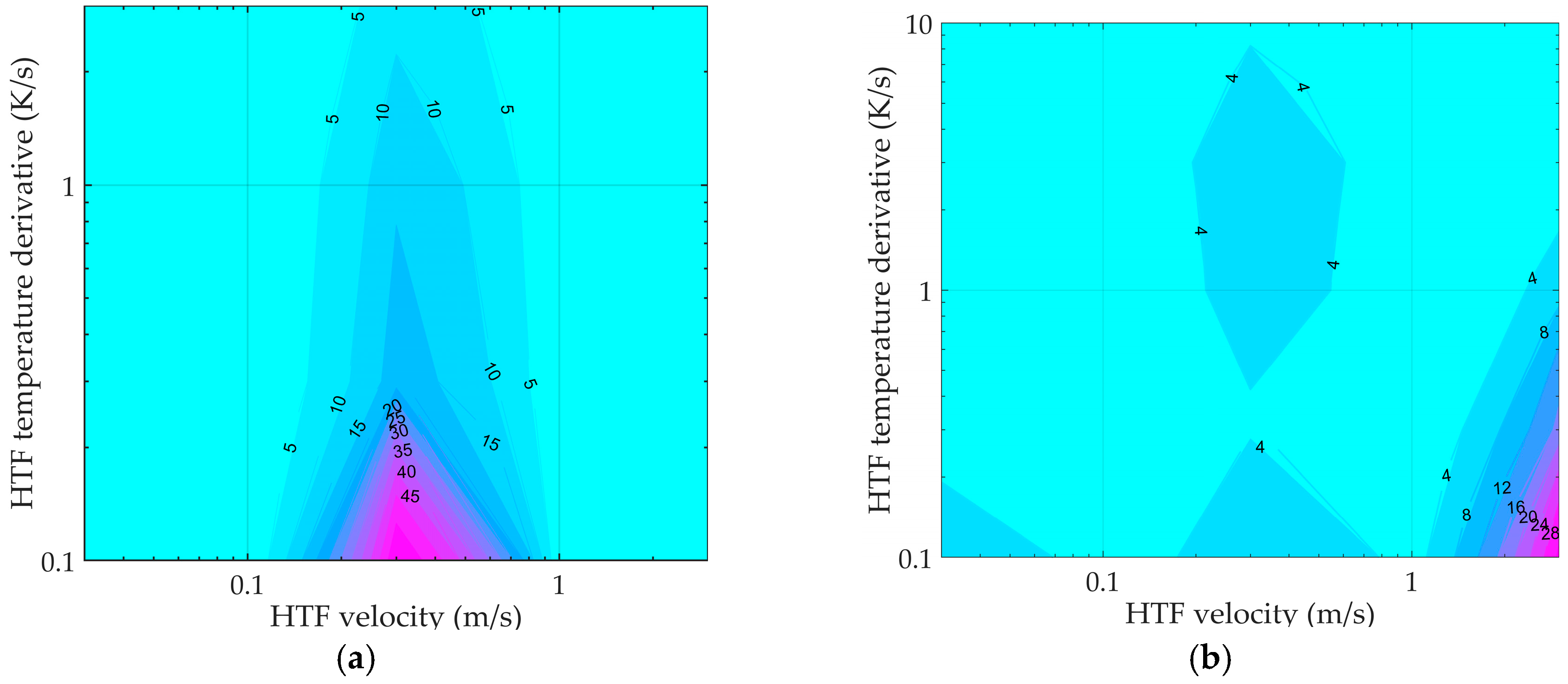
As regards the global time step, it is fixed at 10 s, which allows to prevent any temperature leveling due to the thermal inertia of the pipelines. All the tubes have an internal diameter of 6 cm and a thickness of the insulating material of 3 cm. In order to limit the redundancy of the results, the fluid regimes are shown with reference to the following sections: (i) the outlet of the solar field (pipe 12 m long) and (ii) the outlet of the organic Rankine cycle system (pipe 5 m long). For both tubes the time derivative of the outlet temperature and the oil flow rate are calculated. Figure 1a,b report for both the sections previously mentioned the HTF regimes, in percent of the total time.
According to the contour plots depicted in Figure 1a,b, most of the operation occurs in a circumscribed region with rr < 1 K/s and 0.1 m/s < u < 0.1 m/s or u > 1 m/s, depending on the considered section.
Later on, the performance of the four models considered in this study are assessed and compared. The fluid is supposed to increase its temperature from 300 K up to 600 K inside a pipeline 10 m long. A sensitivity analysis is carried out by varying the slope of the temperature increase and the HTF velocity. Figure 2 shows an example of the response time of the four models under investigation with a rr = 1 K/s and 0.5 m/s.
It is worth noticing that the linear approximation of the temperature profile along the pipe length leads to an unphysical decrement of the outlet temperature during the initial transitory for the 0D and the 1D radial model. In particular, this is more relevant with low flow rate and strong increase of the inlet temperature, or rather when the temperature gradient along the axial direction is high. On the basis of the results attained by the 2D model, the deviations of the other models are evaluated as reported in Figure 3. The good accuracy of the 1D longitudinal model with the results of the 2D model for HTF velocities higher than 0.1 m/s is evident at any temperature gradient as shown in Figure 3a.
On the contrary, it cannot be stated the same for the 1D radial model. In fact, for HTF velocities in the range 0.1–1 m/s significant deviations occur on the predicted output temperature when rr > 3, as reported in Figure 3b. Hence, the assumption of a linear temperature distribution along the tube length causes a consistent error in the evaluation of the temperature profile. Eventually, the lumped model exhibits good accuracy only when the axial gradient is low, that is when the temperature increase is smooth and/or the fluid has a high velocity, as shown in Figure 3c.
Therefore, with reference to the operation of the Innova plant (see Figure 1), characterized by rr < 1 K/s and u > 0.1 m/s for most of the time, only the lumped model does not agree with the results of the most detailed 2D model, with the exception of HTF velocities > 1 m/s. The 1D radial model, instead, can lead to unrealistic values in the case of high temperature derivatives (rapid changes of direct normal irradiance (DNI)) at 0.1 m/s < u < 1 m/s. Moreover, the latter one has no advantage in terms of CPU time with respect to the more accurate 1D longitudinal model, as shown in Figure 4.
In light of this, the most suitable model for dynamic simulations of the pipelines in small-scale mid-temperature solar CHP plants is the 1D longitudinal model. Therefore, in order to estimate the influence of the transient behavior of the pipelines on the dynamic simulation of small-scale concentrated solar CHP plants, this model is implemented for the case of the integrated Innova Microsolar plant in the Simulink platform. Indeed, this work is part of a more extended activity aimed at developing a smart simulator of small-scale solar ORC CHP systems to be integrated into the built environment. Hence, the energy performances of the plant obtained by implementing the 1D longitudinal model of the pipelines are compared with those considering the tube model of the Simscape library [21]. Compared to the Simscape library model of the tube, the proposed 1D longitudinal model is able to adjust its internal time step based on the Courant–Friedrich condition calculated at the inlet of the tube and fixed at 0.8. However, in the case of high HTF flow rates such as at the nominal operating conditions of the linear Fresnel reflectors solar field (about 3 kg/s), the 1D longitudinal model entails undesired computational efforts due to the significant decrease of the internal time step. Moreover, in the case of the 1D longitudinal model, the performances of the integrated plant are evaluated both for one node and 20 nodes, thus assessing their impact on the annual energy results, as reported in Table 3:
Where TE,out LFR and TE,loss LFR are the thermal energy output and losses from the LFR, TE, in TES is the thermal energy input to the TES, TE tube loss are the thermal energy losses from the tubes, TE,in ORC is the thermal energy input to the TES, EE,out ORC the electric energy output by the ORC and Eff ORC the electric efficiency of the ORC unit.
Since the Simscape library model of the tube is a simplified lumped model, some relevant discrepancies of the performances occur compared with those obtained using the 1D Simulink model. In particular, in the case of the Simscape model the pipeline losses are 7.91% higher, thus leading to a lower electric energy production of about 6.3% (1.78 × 10⁷ kJ compared to 1.93 × 10⁷ kJ of the Simulink 1N). This is mostly due to the lower running time of the plant (9.42% lower). On the other hand, the ORC unit works most of the time at operating conditions having higher electrical efficiencies and as a result the mean electric efficiency is 3% higher (6.65% compared to 6.44% of the Simulink 1N). The CPU time in Table 3 is measured on a workstation equipped with 32 GB of RAM and the Intel Xeon E5530 @ 2.4 Ghz processor whilst the code is able to use a single thread only.
As regards the thermal discretization of the pipeline in the 1D longitudinal model, it does not exhibit significant variation in the aggregated energy values. Indeed, all the annual results are within 1% of deviation. However, the same cannot be said for the monthly average energies where significant relative differences occur, as depicted in Figure 5b.
Indeed, during the winter period all the subsystems work at off-design conditions; the LFR solar field usually operates at low flow rates and in the case of high DNI, the longitudinal thermal gradient along the pipelines increases. This can be easily appreciated in Figure 6 which reports the HTF regime at ORC outlet (Figure 6a) and LFR outlet (Figure 6b) for the winter month of December. Compared to the contour plots of Figure 1 that refer to the annual simulation, it can be noticed the lower fluid flow rates especially at the LFR outlet which affect the performance of the whole plant. In the case of low DNI, the oil from the LFR solar field often bypasses the TES and goes directly to the ORC unit, thus making the fluid regime at the ORC outlet and LFR outlet more similar (see Figure 6).
Eventually, the discrepancies of the plant performances between the 1D longitudinal model with 20 thermal nodes and the simplified Simscape model are shown for typical days of operation in winter time. In particular, Figure 7 shows the temperature and flow-rate profiles for a typical day in January while Figure 8 shows December. In this case, the low solar radiation together with the very low oil flow rates cause higher longitudinal thermal gradients along the pipelines and as a consequence the discrepancies between the two models are more evident. According to the plant operation modes the high-mass flow rates (about 3 kg/s) occur when the TES is in operation (charging or discharging) depending on the solar radiation. For further details on the plant operation modes, interested readers are invited to see paper [15].
4. Discussion
In general, the analysis confirms that the operation of a solar ORC system (in terms of operating hours and electric efficiency) is significantly affected by the pipelines representation model.
The developed thermodynamic model of the ORC unit limits the operation of the system at inlet thermal power below 25 kWth and fixes a minimum inlet temperature of about 130 °C. This means a continuous regulation of the input parameters to agree with the fixed constraints, especially at low flow rates. As a result, the higher spatial resolution of the thermal profile provided by the most accurate pipeline model determines greater fluctuations of the temperatures, as shown in Figure 7 and Figure 8. Moreover, the damping effects on the inlet parameters of the ORC subsystem typical of the lumped model disappear. Another implication in adopting an elevated number of thermal nodes is the consequent sharpness of the temperature fronts, as depicted in Figure 7. On the contrary, the presence of the crossing delay time cannot be appreciated here, also because of the high-mass flow rate of the HTF.
Considering the monthly averaged energy values (Figure 5), the solar CHP system works mainly at nominal conditions during the summer time when the energy production occurs for a prolonged time and as a consequence the influence of the thermal gradient can be neglected. On the contrary, in winter season the HTF regime reduces considerably and, despite this, it does not affect the thermal losses, as shown in Figure 5a; the sharpened fronts of the temperature profile have significant influence on the performance of the different subsystems, especially when their operation at off-design conditions is poor. For instance, the ORC system regulates often according to the changing inlet power and temperature and as a consequence it is subject to higher thermal gradients which result in reduced electric energy production. On the other hand, with the Simscape model of the tube the thermal losses of the pipelines are overestimated when compared with those of the Simulink 1N model (see Figure 5b), for two reasons mainly: first, the external convective coefficient of the tube is fixed at 20 W/m2∙K, while in the Simulink models it depends also on the wind velocity (Equations (9) and (13)); second, the thermal conduction of the insulating material is fixed in the middle of the operating conditions, equal to 0.07 W/m∙K (see Table 2), whilst in the 1D longitudinal model it depends on the mean temperature between the HTF and the external ambient for each thermal node, thus reflecting the real operating conditions of the tubes.
Adding extra thermal nodes does not provide any gain in accuracy if the HTF flow rate is high, since it levels the temperature gradient in the axial direction. This behavior can be easily appreciated in Figure 3c where the lumped model provides the same results as those of the 2D model for the case of HTF velocities higher than 1 m/s and a temperature gradient rr < 1 K/s. In terms of computational efforts, the lumped model exhibits by far the best performance especially at high HTF velocities, as shown in Figure 4. Indeed, it is basically independent from the mass flow rate, unlike the other models which need to adjust their internal time step. Despite the global computational time of the simulations depending not only on the model of the pipelines but also on those of the different subsystems (LFR, TES, ORC etc.), using the Simulink 20N model the CPU time is more than twice the computational time of the simulations using the Simscape or the Simulink 1N model, as shown in Table 3.
In conclusion, an hybrid model able to switch from a 1D longitudinal model to a 0D model with delay according to the fluid flow rate is the best compromise to obtain results accurate enough and to reduce the high computational effort due to the small internal time step at high flow rates in the case of 1D models.
5. Conclusions
Dynamic thermal distribution networks, as those in concentrated solar cogeneration and trigeneration plants, need an appropriate modeling of the pipelines network. In this study the comparison of four different mathematical models of the tubes is carried out on the basis of the fluid regime (in terms of temperature derivative at the inlet and flow velocity) typical of the Innova Microsolar plant. Such comparison shows that:
- ■
- the 1D radial model entails significant deviations on the predicted output temperature for HTF velocities in the range 0.1–1 m/s when rr > 3;
- ■
- the 1D longitudinal model is in good agreement with the results of the 2D model at any rr for HTF velocities higher than 0.1 m/s;
- ■
- the lumped model agrees with the results of the 2D model at HTF velocities >1 m/s.
Therefore, whenever high-longitudinal thermal gradients occur in the pipelines of complex energy systems, the calculated thermal losses as well as the dynamic response of the whole system can vary considerably based on the mathematical model used. With respect to the performances of the small-scale concentrated solar CHP plant of the Innova Microsolar project, the discrepancies of the predicted performances of the plant between the lumped model of the Simscape library and the 1D longitudinal model become significant during winter season. In particular, due to the net temperature fronts obtained with the more accurate model of the pipelines, the ORC unit can better exploit the energy input. As a consequence, the annual electrical energy production of the ORC unit is more than 6%. On the other hand, whenever the longitudinal thermal gradient inside the pipeline is negligible, a lumped model for dynamic simulations is accurate enough, thus significantly reducing the computational time without losing accuracy.
Therefore, the analysis carried out has allowed assessment of the soundness of the different models of the tubes for small-scale concentrated solar ORC systems, and to conclude that an hybrid model able to switch from a 1D longitudinal model to a 0D model, with delay based on the fluid flow rate, is the best compromise to obtain results accurate enough whilst limiting the computational efforts. Hence, this approach will be implemented in the future in the smart simulator of small-scale solar ORC CHP systems the authors are going to develop.
Author Contributions
Conceptualization, R.T.; methodology, E.H. and R.T.; software, R.T.; writing—original draft preparation, R.T. and L.C.; writing—review and editing, L.C. and L.D.Z.; supervision, E.H., L.C. and L.D.Z.; funding acquisition, L.C. All authors have read and agreed to the published version of the manuscript.
Funding
This research is part of the Innova Microsolar Project that was funded by the European Union’s Horizon 2020 Research and Innovation Programme (grant agreement No 723596). The APC was funded by the European Union’s Horizon 2020 Research and Innovation Programme (grant agreement No 723596).
Conflicts of Interest
The authors declare no conflict of interest.
Nomenclature
| A | internal cross section area of the tube (m2) |
| c | specific heat at constant pressure (J/kg·K) |
| CHP | combined heat and power |
| D | diameter (m) |
| DH | district heating |
| DNI | direct normal irradiance (W/m2) |
| EE | electrical energy |
| frD | Darcy friction coefficient |
| g | gravity (m2/s) |
| h | convective coefficient (W/m2·K) |
| k | thermal conductivity (W/m·K) |
| L | length of the tube (m) |
| LFR | linear Fresnel reflectors |
| ORC | organic Rankine cycle |
| p | pressure (Pa) |
| Pr | Prandtl number |
| R | thermal resistance (K·m/W) |
| r | radius (m) |
| rr | angular coefficient of the temperature increase/decrease (K/s) |
| Ra | Rayleigh number |
| Re | Reynolds number |
| S | internal “wetted” area of the tube (m2) |
| T | temperature (K) |
| TE | thermal energy |
| TES | thermal energy storage |
| t | time (s) |
| u | velocity of the heat transfer fluid (m/s) |
| x | longitudinal axis |
| heat transfer rate (W/m) | |
| Subscripts and superscripts | |
| 1 | internal part of the tube |
| 2 | external part of the tube |
| 2-amb | mean properties between the external part of the tube and the external ambient |
| amb | external ambient |
| conv,int | internal convective |
| conv,ext | external convective |
| cond | conductive |
| del | delay |
| ext | external |
| HTF | heat transfer fluid |
| i | i-th cross section along x direction |
| in | inlet |
| int | internal |
| ins | insulating material |
| j | j-th along the radial direction |
| k | k-th time step |
| loss | losses |
| Nu | Nusselt number |
| oil | diathermic oil |
| out | outlet |
| R | radius |
| sc | Simscape |
| Steel | stainless steel metal |
| th | thermal |
| w | wall |
| Greek symbols | |
| ∆x | finite space difference along the longitudinal direction x (m) |
| ∆r | finite space difference along the radial direction (m) |
| ∆t | finite time difference (s) |
| α | thermal diffusivity (m2/s) |
| β | thermal expansion coefficient (1/K) |
| ν | kinematic viscosity (m2/s) |
| η | efficiency |
| ρ | density (kg/m3) |
References
- Clean Energy for All Europeans—Publications Office of the EU. Available online: https://op.europa.eu/en/publication-detail/-/publication/b4e46873-7528-11e9-9f05-01aa75ed71a1/language-en?WT.mc_id=Searchresult&WT.ria_c=null&WT.ria_f=3608&WT.ria_ev=search (accessed on 27 December 2019).
- Energy Performance of Buildings Directive Energy. Available online: https://ec.europa.eu/energy/en/topics/energy-efficiency/energy-performance-of-buildings/energy-performance-buildings-directive (accessed on 27 December 2019).
- Werner, S. International Review of District Heating and Cooling. Energy 2017, 137, 617–631. [Google Scholar] [CrossRef]
- Persson, U.; Werner, S. District Heating in Sequential Energy Supply. Appl. Energy 2012, 95, 123–131. [Google Scholar] [CrossRef]
- van der Heijde, B.; Fuchs, M.; Ribas Tugores, C.; Schweiger, G.; Sartor, K.; Basciotti, D.; Müller, D.; Nytsch-Geusen, C.; Wetter, M.; Helsen, L. Dynamic Equation-Based Thermo-Hydraulic Pipe Model for District Heating and Cooling Systems. Energy Convers. Manag. 2017, 151, 158–169. [Google Scholar] [CrossRef] [Green Version]
- Dénarié, A.; Aprile, M.; Motta, M. Heat Transmission over Long Pipes: New Model for Fast and Accurate District Heating Simulations. Energy 2019, 166, 267–276. [Google Scholar] [CrossRef]
- del Hoyo Arce, I.; Herrero López, S.; López Perez, S.; Rämä, M.; Klobut, K.; Febres, J.A. Models for Fast Modelling of District Heating and Cooling Networks. Renew. Sustain. Energy Rev. 2018, 82, 1863–1873. [Google Scholar] [CrossRef]
- Chertkov, M.; Novitsky, N.N. Thermal Transients in District Heating Systems. Energy 2018, 184, 22–33. [Google Scholar] [CrossRef] [Green Version]
- Wang, H.; Meng, H. Improved Thermal Transient Modeling with New 3-Order Numerical Solution for a District Heating Network with Consideration of the Pipe Wall’s Thermal Inertia. Energy 2018, 160, 171–183. [Google Scholar] [CrossRef]
- Hudson, J.; Sweby, P.K.; Baines, M.J. Numerical Techniques for Conservation Laws with Source Terms. Ph.D. Dissertation, University of Reading, Reading, UK, 2001. [Google Scholar]
- Wang, Y.; You, S.; Zhang, H.; Zheng, X.; Zheng, W.; Miao, Q.; Lu, G. Thermal Transient Prediction of District Heating Pipeline: Optimal Selection of the Time and Spatial Steps for Fast and Accurate Calculation. Appl. Energy 2017, 206, 900–910. [Google Scholar] [CrossRef]
- Taccani, R.; Obi, J.B.; De Lucia, M.; Micheli, D.; Toniato, G. Development and Experimental Characterization of a Small Scale Solar Powered Organic Rankine Cycle (ORC). Energy Procedia 2016, 101, 504–511. [Google Scholar] [CrossRef] [Green Version]
- Manfrida, G.; Secchi, R.; Stańczyk, K. Modelling and Simulation of Phase Change Material Latent Heat Storages Applied to a Solar-Powered Organic Rankine Cycle. Appl. Energy 2016, 179, 378–388. [Google Scholar] [CrossRef] [Green Version]
- Villarini, M.; Tascioni, R.; Arteconi, A.; Cioccolanti, L. Influence of the Incident Radiation on the Energy Performance of Two Small-Scale Solar Organic Rankine Cycle Trigenerative Systems: A Simulation Analysis. Appl. Energy 2019, 242, 1176–1188. [Google Scholar] [CrossRef]
- Cioccolanti, L.; Tascioni, R.; Arteconi, A. Mathematical Modelling of Operation Modes and Performance Evaluation of an Innovative Small-Scale Concentrated Solar Organic Rankine Cycle Plant. Appl. Energy 2018, 221, 464–476. [Google Scholar] [CrossRef]
- Wei, L.; Lei, Q.; Zhao, J.; Dong, H.; Yang, L. Numerical Simulation for the Heat Transfer Behavior of Oil Pipeline during the Shutdown and Restart Process. Case Stud. Therm. Eng. 2018, 12, 470–483. [Google Scholar] [CrossRef]
- Frank, P.; Incropera, D.P.D. Fundamentals of Heat and Mass Transfer; la University of Michigan: Ann Arbor, MI, USA, 1990. [Google Scholar]
- Innovative Micro Solar Heat and Power System for Domestic and Small Business Residential Buildings. Available online: http://innova-microsolar.eu/ (accessed on 8 July 2019).
- Mahkamov, K.; Pili, P.; Manca, R.; Pula, E.; Sardinia, I.A.; Leroux, A.; Charles, M.; Enogia, S.A.S.; Lynn, K.; Mullen, D.; et al. Development of a Small Solar Thermal Power Plant for Heat and Power Supply to Domestic and Small Business Buildings. Power Energy 2018. [Google Scholar] [CrossRef]
- Vivian, J.; De Uribarri, P.M.Á.; Eicker, U.; Zarrella, A. The Effect of Discretization on the Accuracy of Two District Heating Network Models Based on Finite-Difference Methods. Energy Procedia 2018, 149, 625–634. [Google Scholar] [CrossRef]
- Rigid Conduit for Fluid Flow in Thermal Liquid Systems—MATLAB—MathWorks Italia. Available online: https://it.mathworks.com/help/physmod/simscape/ref/pipetl.html (accessed on 4 January 2020).
Figure 1.
Fluid regime at organic Rankine cycle (ORC) outlet (a) and at linear Fresnel reflectors (LFR) outlet (b), in percent of total time for an annual simulation. HTF is heat transfer fluid.
Figure 1.
Fluid regime at organic Rankine cycle (ORC) outlet (a) and at linear Fresnel reflectors (LFR) outlet (b), in percent of total time for an annual simulation. HTF is heat transfer fluid.

Figure 2.
Response time test of the four models with rr = 1 K/s and HTF velocity = 0.5 m/s.

Figure 3.
(a) Relative error in the one-dimensional (1D) longitudinal model; (b) Relative error in the 1D radial model; (c) Relative error in the zero-dimensional (0D) model.
Figure 3.
(a) Relative error in the one-dimensional (1D) longitudinal model; (b) Relative error in the 1D radial model; (c) Relative error in the zero-dimensional (0D) model.

Figure 4.
Speed up vs. two-dimensional (2D) model.

Figure 5.
(a) Simscape/Simulink 1N monthly averaged energy variations; (b) Simulink 1N/20N monthly averaged energy variations.
Figure 5.
(a) Simscape/Simulink 1N monthly averaged energy variations; (b) Simulink 1N/20N monthly averaged energy variations.

Figure 6.
HTF regime at ORC outlet (a) and at LFR outlet (b) in percent of total time (December).

Figure 7.
Temperature and flow rate at the outlet of the LFR and ORC.

Figure 8.
Temperature and flow rate at the outlet of the LFR and ORC. DNI is direct normal irradiance.
Figure 8.
Temperature and flow rate at the outlet of the LFR and ORC. DNI is direct normal irradiance.


Table 1.
Values of C and m with Reynolds number.
| Re2 | C | m |
|---|---|---|
| 1–40 | 0.75 | 0.4 |
| 40–103 | 0.51 | 0.5 |
| 103–2 × 10⁵ | 0.26 | 0.6 |
| 2 × 10⁵–106 | 0.076 | 0.7 |
Table 2.
Thermal properties of PROPOX PS964 mineral wool (EN ISO 8497).
| Temperature (°C) | Thermal Conductivity (W/m∙K) |
|---|---|
| 50 | 0.042 |
| 100 | 0.049 |
| 150 | 0.059 |
| 200 | 0.071 |
| 250 | 0.086 |
| 300 | 0.105 |
Table 3.
Annual energy results.
| Parameter | Simscape | Simulink 1N | Simulink 20N |
|---|---|---|---|
| TE,out LFR (kJ) | 3.86 × 10⁸ | 3.87 × 10⁸ | 3.87 × 10⁸ |
| TE,loss LFR (kJ) | 7.96 × 10⁷ | 7.71 × 10⁷ | 7.73 × 10⁷ |
| TE,in TES (kJ) | 9.61 × 10⁷ | 1.00 × 10⁸ | 1.01 × 10⁸ |
| TE,in ORC (kJ) | 2.99 × 10⁸ | 2.99 × 10⁸ | 2.98 × 10⁸ |
| TE tube loss (kJ) | 6.58 × 10⁷ | 6.06 × 10⁷ | 6.11 × 10⁷ |
| EE,out ORC (kJ) | 1.78 × 10⁷ | 1.90 × 10⁷ | 1.93 × 10⁷ |
| Eff ORC (%) | 6.65 | 6.44 | 6.58 |
| Time on (s) | 1.09 × 10⁷ | 1.19 × 10⁷ | 1.19 × 10⁷ |
| CPU time (s) | 2.30 × 10⁴ | 3.01 × 10⁴ | 7.95 × 10⁴ |
© 2020 by the authors. Licensee MDPI, Basel, Switzerland. This article is an open access article distributed under the terms and conditions of the Creative Commons Attribution (CC BY) license (http://creativecommons.org/licenses/by/4.0/).
Share and Cite
MDPI and ACS Style
Tascioni, R.; Cioccolanti, L.; Del Zotto, L.; Habib, E. Numerical Investigation of Pipelines Modeling in Small-Scale Concentrated Solar Combined Heat and Power Plants. Energies 2020, 13, 429. https://doi.org/10.3390/en13020429
AMA Style
Tascioni R, Cioccolanti L, Del Zotto L, Habib E. Numerical Investigation of Pipelines Modeling in Small-Scale Concentrated Solar Combined Heat and Power Plants. Energies. 2020; 13(2):429. https://doi.org/10.3390/en13020429
Chicago/Turabian StyleTascioni, Roberto, Luca Cioccolanti, Luca Del Zotto, and Emanuele Habib. 2020. "Numerical Investigation of Pipelines Modeling in Small-Scale Concentrated Solar Combined Heat and Power Plants" Energies 13, no. 2: 429. https://doi.org/10.3390/en13020429
Note that from the first issue of 2016, this journal uses article numbers instead of page numbers. See further details here.