Distributed Economic Dispatch Scheme for Droop-Based Autonomous DC Microgrid


1
Jiangsu Engineering Laboratory of Gas-Electricity Integrated Energy, Nanjing Normal University, Nanjing 210023, China
2
Jiangsu Key Laboratory of Smart Grid Technology and Equipment, Southeast University, Nanjing 210096, China
*
Author to whom correspondence should be addressed.
Energies 2020, 13(2), 404; https://doi.org/10.3390/en13020404
Submission received: 28 October 2019
/
Revised: 8 January 2020
/
Accepted: 10 January 2020
/
Published: 14 January 2020
(This article belongs to the Special Issue Advanced Control in Microgrid Systems)
Abstract
:In this paper, a distributed economic dispatch scheme considering power limit is proposed to minimize the total active power generation cost in a droop-based autonomous direct current (DC) microgrid. The economical dispatch of the microgrid is realized through a fully distributed hierarchical control. In the tertiary level, an incremental cost consensus-based algorithm embedded into the economical regulator is utilized to search for the optimal solution. In the secondary level, the voltage regulator estimating the average voltage of the DC microgrid is used to generate the voltage correction item and eliminate the power and voltage oscillation caused by the deviation between different items. Then, the droop controller in the primary level receives the reference values from the upper level to ensure the output power converging to the optimum while recovering the average voltage of the system. Further, the dynamic model is established and the optimal communication network topology minimizing the impact of time delay on the voltage estimation is given in this paper. Finally, a low-voltage DC microgrid simulation platform containing different types of distributed generators is built, and the effectiveness of the proposed scheme and the performance of the optimal topology are verified.
1. Introduction
Microgrid is a new form of grid consisting of distributed generations (DGs), energy storages, loads and power electronic devices, which is considered as a solution for flexible and reliable integration of renewable energy resources into the grid [1,2]. Compared with alternating current microgrid (AC MG), direct current microgrid (DC MG) has attracted more attentions due to the advantages that it can overcome some disadvantages of AC system, such as transformer inrush current, frequency synchronization, reactive power flow, power quality issues, etc. Therefore, DC microgrid is widely used in data centers and IT facilities, where the load is DC in nature [3,4]. Similar to AC microgrid, in order to improve the reliability of power supply, DC load is usually supplied by multiple distributed generators operated in parallel when in autonomous operation mode. However, unlike the synchronous generators in transmission network, there are different types of DGs in microgrid, such as internal combustion engines, dispatchable clear resources (fuel-cell), and non-dispatchable renewable resources (solar, wind turbines) [5]. Because of different generation costs of these distributed generators, the traditional way of power sharing based on capacity leads to higher operation cost.
To minimize the total operation cost, economic dispatch problem (EDP) is presented. The optimal economic dispatch objective of autonomous microgrid is to minimize its operation cost, while satisfying both equality and inequality constraints in the MG. Conventionally, the economic dispatch scheme is realized by centralized method, where the control decisions are performed based on global information, which is collected by microgrid central controller (MGCC) using an extensive communication network between MGCC and DGs [6,7,8]. However, the reliability of centralized method is poor because of the failure of the center node or link, and the capability of plug and play is weakened by centralized communication. Therefore, the decentralized and distributed methods are more practical for microgrid than centralized control because of their reliabilities, flexibilities, as well as sparse communication channels [9].
It is known that the operation of droop-based microgrid requires no MGCC and communication network, thus some previous literatures have discussed the decentralized economic dispatch scheme for droop-based microgrid, in which the simplicity and decentralized nature of the droop control are retained [5,10,11,12]. In [5,10], a cost-based droop control strategy has been proposed based on the generation costs of distributed generators in ac microgrid that the outputs of high-cost generators are less, while that of low-cost generators are more instead of equal sharing. Later, similar works were carried out in DC MG [11,12]; however, because of the impedance of the power line, the bus voltages of the DC MG are different from each other so that the power distribution accuracy is not well according to their strategies. Additionally, the control parameters of the decentralized economic dispatch strategies mentioned above need to be designed based on the global information, thus the plug and play capability is weakened. A fully distributed control strategy for frequency-power droop type DGs, which allowed all DGs share loads according to their generation costs was proposed in [13], however, the stability of the system and capability of plug and play were not demonstrated. Considering the fuel cost, maintenance cost, and emission penalties of DGs, a nonlinear cost-based droop scheme, where the incremental costs of DGs were embedded into, was developed to achieve a reduction in generation cost, and a linear cost-based droop scheme was proposed later to decrease the complexity of the nonlinear droop control in [14]. Further, the power limits of DGs were taken into account when developing the decentralized economic dispatch scheme in [15].
Compared with the centralized and decentralized method, P2P sparse network based distributed control and optimization methods have drawn more attentions [16,17,18,19]. Various algorithms have been developed recently to solve the EDP in a distributed way. For example, a distributed dynamic programming-based strategy considering generation limits and ramping rate limits was proposed for economic dispatch in smart grid in [20]. Reference [21] proposed a two-stage distributed control strategy for autonomous microgrid, where the sub-gradient-based consensus algorithm was developed to recover frequency and minimize total cost. Considering the power losses and generation limits, a distributed auction-based algorithm was provided in [22], where the EDP was formulated as a nonconvex model. Recently, the distributed consensus algorithms have found their applications in many previous literatures [23,24,25,26], and the incremental cost of DGs is often chosen as the consensus variable to solve the EDP according to the equal incremental cost principle. Additionally, the incremental welfare consensus algorithm with the consideration of responsive loads was proposed further in [27]. However, the dynamics of the converters in these literatures are neglected, and the practicability is not taken into account. For droop-based autonomous DC microgrid, the distributed method was also used for EDP solving [28,29]. In reference [28], the consensus method was utilized to generate the voltage correction term and reference current respectively to ensure the optimal operation for DC microgrid, while the average voltage was recovered at the same time. In this reference, the stability of the system and the convergence performance associating with different control parameters were analyzed. However, the factors affecting flexible operation should be considered further, such as topology changing, plug and play, etc. Unlike [28], in [29], the voltage regulator and optimizer embedded with consensus algorithm were used to adjust the voltage set points to match the incremental costs and recover the average voltage. The power limits are considered and analyzed in detailed. However, the flexibility of distributed control needs further verification.
As discussed above, lots of schemes have been proposed to solve the EDP, which can be classified into two main categories.
- Decentralized economic dispatch scheme that requires local information only. This type of optimal control is less expensive because no communication is needed. However, the lack of common information (such as the common bus voltage in DC MG) leads to the challenge in utilizing all available resources in the network. Additionally, the power and voltage oscillation may happen, if every DGs regulate their output power just taking their own generation costs into account.
- Distributed economic dispatch scheme that requires only local computation and information exchange among some neighboring units through a sparse communication network. Based on the well-designed distributed schemes, the EDP can be solved by multiple distributed controllers working in parallel, which increases the reliability, flexibility, and scalability of the system. Therefore, the distributed manners are considered as promising options for the optimal control and management of microgrid. However, there are also many problems remained to be solved before the distributed schemes become more practical for microgrid, such as time delay, the capability of plug and play, the choice of communication topology, and so on.
Based on the previous researches, a distributed economic dispatch scheme considering power limit for droop-based autonomous DC microgrid is developed to achieve the minimal operation cost in this paper. The proposed scheme contains three control levels, namely, the droop controller works as the primary control to maintain the power balance with source/load transient and to ensure the voltage stable. The secondary control, embedded with a voltage regulator, uses the discrete consensus algorithm to estimate the average voltage of the system and recover the voltage deviation caused by primary control without oscillation. The tertiary control, embedded with an economical regulator, regulates the output power of different DGs to ensure the optimal operation of microgrid. Based on the consensus algorithm, the scheme works in a fully distributed manner without central controller and the communication only occurs between device and its neighbors. Moreover, the dynamic model of the system is established to guide the design of parameters, and the impact of time delay, which will cause the deviation of voltage estimation, is analyzed. Finally, an optimal communication topology is selected to minimize the impact of delay. Compared with the existing economic dispatch scheme, the key contributions of this paper are:
- The proposed distributed scheme can resolve the problems of power sharing accuracy and voltage oscillation caused by the estimation errors, which cannot be effectively solved by decentralized methods.
- The economical regulator updates the control signal with the newest information in each iteration step, instead of requiring the achievement of consensus. Therefore, the convergence speed of the proposed scheme is faster than the traditional consensus-based economic dispatch scheme, which is important for large-scale system.
- To support the flexible operation of DGs, the proposed scheme also adds the capability of plug and play into cyber layer to promote the reliability and scalability of the distributed scheme.
- The impact of time delay on the voltage estimation is analyzed in detail, and the capability of inhibiting oscillation caused by time delay is used to optimize the topology of the sparse communication network.
The rest of paper is organized as follows: Section 2 introduces the preliminaries, including problem formation and discrete consensus algorithm. The proposed distributed economic dispatch scheme is presented in Section 3. Section 4 optimizes the communication topology based on the analysis of time delay. The simulation case study is carried out in Section 5 to validate the performance of the scheme. Finally, Section 6 presents concluding remarks.
2. Preliminaries
2.1. Problem Formation of EDP
There are different DGs in microgrid, such as micro-turbines, diesel generators, fuel cells, solar cells, wind turbines, and so on. The DGs are usually classified into three types, namely, combustion engine, schedulable clear resource and non-schedulable renewable resource. The cost functions of these distributed generators are decided by the type of DGs. For example, if the generation is a diesel generator driven by an internal combustion engine or an electric generator driven by microturbine, its generation cost function usually consists of fuel cost, maintenance cost, and emission penalty, which can be described as [5] follows:
where Km, Kf, Kξ are the coefficients of maintenance cost, fuel cost, and emission penalty. a, b, and c are coefficients of the fuel consumption curve of the DG, which can be achieved by fitting the experiment data. d, e, f, ξ, and ρ are coefficients of generator emission characteristics [30]. However, the emission penalty coefficient Kξ is much smaller than another two, therefore the emission penalty part is neglected in the paper, and the remaining part can be organized as a second-order quadratic function. Additionally, for clean energy source such as fuel cell, its generation cost function only consists of fuel cost and maintenance cost, thus the type of cost function is the same with the above one.
Another type of DG is non-schedulable renewable resource, such as photovoltaic generation and wind generation, the cost function of this type usually contains maintenance cost and power loss cost, which can be described as [5] follows:
where Km, Kl are the coefficients of maintenance cost and loss cost respectively. v, u, and w are related to the characteristic of the converter, which decide the loss of renewable energy. As (2) shows, the cost function of this type can be still written to a quadratic function. Thus, in this paper, the cost functions of different DGs are modelled uniformly as follows:
where Pi denotes the output of DGi, Ci represents the cost function for generator i, and ai, βi, γi are cost coefficients decided by the type of DGi. Thereafter, the objective of EDP is defined as minimizing the total operation cost, i.e.,
where PD is the total active load demand in the MG, Ploss is the transmission loss. Pimin and Pimax are the generation limits of DGi, respectively. The EDP formulated in (4) can be solved by the Lagrange multiplier method, and the solution to (4) can be obtained, which is the equal incremental cost principle, and it takes the following forms,
where ∂Ci(Pi)/∂Pi = λi is the incremental cost of DGi, and λop is the optimal incremental cost of DG. The principle in (5) denotes that the total active power generation cost of the MG is minimized, if only the equal incremental cost principle is satisfied.
2.2. Discrete Consensus Algorithm
Consensus algorithms are usually applied to solve disagreements between agents with different dynamics via peer-to-peer communications. Let xi denote the state variable of node i. Node i only communicates with its neighbors, and xi can represent physical quantities such as voltage, current, power, etc. We can say the nodes have reached a consensus if and only if xi = xj for all i, j. Considering the discrete nature of digital communication, the consensus algorithm can be written in discrete form as [31],
where Ni represents the set of adjacent nodes, namely, a node j belongs to Ni if there exists a communication link between it and node i. xi [k] is the consensus state variable of node i at kth iteration. dij is the communication weight, where dij > 0 if node j belongs to Ni and dij = 0, otherwise. The Equation (6) can be rewritten in matrix form as follows:
where Xk and Xk+1 are the vectors of system state variable at the kth and (k + 1)th iterations respectively. D is the communication weight matrix of the system, which consists of dij. Each node will converge to a common value when D is designed as a stochastic matrix and satisfies some necessary conditions in [32]. The common value will be:
where X[0] is the initial state, f is a nonnegative left eigenvector associated with eigenvalue 1 of D that it satisfies the equation: fT1 = 1, 1 = [1,1,…1]T. Specially, if D is a double-stochastic matrix, then, all nodes will converge to the average value of the system, that is,
In actual control systems, the convergence speed of the consensus algorithm is an important index. It is known that the convergence speed is decided by the spectral radius of D defined as follows
where esr(D) is the modulus of the second largest eigenvalue of D, which is decided by the communication network topology. In order to achieve suitable convergence speed, the Metropolis method in [16] is often used to design the D, and the entries in D are calculated according to the network topology,
where ni and nj are the numbers of nodes in Ni and Nj respectively, which are decided by the communication network topology as well.
3. Proposed Distributed Economic Dispatch Scheme
Figure 1 illustrates the proposed distributed hierarchical economic dispatch scheme for the converters in an autonomous DC microgrid, which consists of three control levels.
3.1. Primary Control
The primary control based on droop scheme is used to keep the DC bus voltage stable and share the output power properly. It consists of inner control loop and droop loop. In autonomous DC microgrid, the droop-based loop is used for coordinating the operation of the converters, which adds the virtual resistance to distribute the power among different converters. The droop scheme can be designed as follows:
where, Uref and Uoi* are the system reference voltage and voltage command of converter respectively. Ioi is the output current of converter. The value of virtual resistance Rdi determines the ratio of power sharing of different converters, which is updated by economical regulator in tertiary control level. Additionally, voltage correction term δVi is used to recover the average voltage of the islanded microgrid, and the droop character is shifted along the voltage axis by addition of δVi from the voltage regulator in secondary control level.
As Figure 1 shows, the inner control loop, which consists of two PI controllers, is used to follow the voltage command Uoi* from the droop loop. The bandwidth of this level is designed to be large enough to maintain the power balance of the system while load changes.
3.2. Voltage Regulation in Secondary Control
It is known that the droop scheme in primary level will cause voltage drop inevitably. Reference [3] indicates that in order to improve the power distribution accuracy, the output voltage of each converter should be lower. Therefore, a voltage recovery process is necessary.
In this paper, all converters acquire the average voltage Uave of the DC microgrid via estimation by voltage regulators, which is used as the synchronous regulating variable to improve the dynamic response of the regulation process. Later, the voltage regulator will compare this value with the objective average voltage and the compensation value will be added to Uref to recover the average voltage of the DC microgrid, as shown in Figure 2.
The proposed voltage regulator includes a sample and hold (S/H1) module and a PI controller. The sample cycle of S/H1 is TS/H1, which is decided by a clock installed in the regulator. Additionally, the communication period is Ts, and TS/H1 = NTs. It means that S/H1 will not sample the new voltage data until the voltage consensus iteration process finishes. It is noting that the number of iteration N before converging is decided by the topology of the communication network, thus, N can be chosen offline. The voltage regulation procedure then can be described as follows.
When t = mNTs, m = 0, 1, 2, …, the voltage regulator samples local voltage Uoi and the output of S/H1 is Uoi[mNTs] abbreviated as Uoi[m]. Then, Uoi[m] is given to Ũi[0], which is the initial value used to estimate the average voltage of the microgrid. From then on, each converter starts to communicate with its neighbors to estimate the average voltage of the microgrid according to consensus algorithm, and its update cycle is synchronized with communication cycle. The consensus iteration process according to the message received from its neighbors can be described as follows,
where dv_ij is the communication weight used in voltage regulator, Ũi[k] and Ũi[k + 1] are the estimation values at the kth and (k + 1)th iterations respectively. After limited iterations N, the process (13) will direct Ũi to the average voltage of the DC microgrid. That is, each voltage regulator in secondary level will get this value Uave. It is worth noting that the number of iteration N before converging is decided by the topology of the communication network, thus, N can be chosen offline. At last, each voltage regulator compares this average voltage Uave with the objective value Uave_op, and the mismatch is passed through a PI controller to generate the compensation value δVi, as shown below:
As aforementioned analysis, the secondary voltage control cycle is NTs. When t = (m + 1)NTs, each voltage regulator starts to sample again and repeats the consensus iteration process (13) and voltage regulation (14). Because of the existence of secondary voltage regulator, the average voltage of the DC microgrid will be recovered to the objective value. However, when some communication events occur in the information interaction period, such as time delay, (13) will not converge to the common value Uave after N iterations. This will lead to the deviation between δVi, i = 1, 2, …, n, which will cause power and voltage oscillation in turn. Thus, the impact of time delay on voltage estimation is analyzed in Section 4.
3.3. Economical Regulation in Tertiary Control
To overcome the disadvantages of centralized solution indicated by (4), incremental cost consensus algorithm is applied to develop a distributed solution to minimize the total operation cost of DC microgrid. An economical regulator is then used to provide objective virtual resistance Rdi* for the primary droop control, by solving EDP with the proposed algorithm, as shown in Figure 3. The economical regulator finds the optimal operational point with an iterative process, whose update cycle is controlled by a clock installed in the tertiary level.
As shown in Figure 3, the economical regulator contains a sample and hold (S/H2) module and some mathematical modules. The sample cycle of S/H2 is TS/H2 = TS. Then, the economic dispatch procedure can be described as follows.
When t = kTS, k = 0, 1, 2, …, the economical regulator samples local voltage Uoi and output current Ioi and calculates the output power Pi[k]. According to equal incremental cost principle, the incremental cost of each DG is chosen as the consensus variable in this proposed distributed iterative approach, which can be calculated by the following equation:
where λi[k] is the local incremental cost achieved in kth sampling, I = 1, 2, …, n. αi and βi are the coefficients of cost function respectively. In the next step, economical regulator i sends this message λi to its neighbors. Because of the bi-direction of the communication network, economical regulator i will also receive the incremental cost information from its neighbors, and calculate the objective incremental cost by
where dp_ij is the communication weight used in economical regulator, λi*[k] is the objective incremental cost, which is moved in the direction of minimizing the total operation cost of the microgrid within the process (16). Then, the objective dispatch reference Pi*[k] in kth iteration corresponding to λi*[k] is
Unlike the PQ control in primary level, the output power of droop-based converter cannot follow the power reference directly. Therefore, in order to control the power indirectly, the virtual resistance is considered. According to the droop characteristic, if the objective output power Pi*[k] is more than Pi[k], then the virtual resistance should be decreased, and vice versa. In this paper, the method adjusting the virtual resistance is designed according to (12) as follows:
where Rdi*[k] is the objective virtual resistance at kth iteration. Note that the method to achieve the objective virtual resistance is not unique. The mismatch between Pi[k] and Pi*[k] can be also used through a PI controller to generate the objective virtual resistance [19]. Then, the virtual resistance in (12) is updated by Rdi*[k] through a low pass filter (LPF), as shown in Figure 1. The first-order low pass filter is used to smoothen the transient process of virtual resistance updating, whose time constant Tm should be larger than the communication cycle Ts.
When t = (k + 1)Ts, the economical regulator samples local voltage and current again and repeats the process (15)–(18). With limited circulations, the incremental costs in all economical regulators will be the same, which indicates the optimal operation of the DC microgrid. The output power and virtual resistance of each converter will converge to the optimal value respectively. The optimal values satisfy the following equation,
The proposed control scheme of economical regulator overcomes the disadvantages of the existed economic droop control, finding the optimal solution of (4) without the information of line impedance and the cost functions of other distributed generators.
3.4. The Consideration of Power Limitation
In the practical low-voltage DC microgrid applications, the power supply distance is usually less than several hundreds of meters that the deviation of different bus voltages are small. Therefore, the voltage constraints are not considered in this paper, only the power constraints are taken into account. It is well-known that the output power of each generator should not be more/less than its maximum/lower generation limits, so the generator reaching its limit must keep the output power at this limit and not to participate in the EDP solving. When considering this problem, the paper changes the communication weight to satisfy the equal incremental cost principle described in (5), which can be described as follows:
Supposing that converter i reaches its limitation Pmax, then the communication weights of this economical regulator will be changed to dp_ii = 1, dp_ij = 0, j∈Ni. In this way, the incremental cost information received from its neighbors will not influence its objective incremental cost according to (16). Then, the objective dispatch reference Pi*[k] keeps to Pmax, and the objective incremental cost keeps to λi* = βi + 2αiPmax. That is, the converter reaching its limitation will not participate in EDP solving at the next time until the total load decreases.
Similarly, in order to make the remaining converters converge to their optimal value, the converter i should send an inform message to its neighbors, and its neighbors will delete converter i from their neighbor sets and change their communication weights again according to (11). Note that the communication weights will not be changed if the converter is not connected with the one reaching its limitation. Thus, the communication weights of converter i and its neighbors g∈Ni can be revised as follows:
where Ng^ is the new neighbor set of the converter g, and ng^ is the numbers of converters in Ng^. Based on the new matrix Dp^, the remaining converters’ incremental costs will converge to the same value, which indicates the optimal operation according to the equal incremental cost principle. The regulation process that the converter reaches its low limit Pmin is the same with that discussed above. Note that the communication weight dv_ij in voltage regulator is not changed, because the converter reaching limit can still participate in voltage regulation.
3.5. The Global Dynamic Model and Parameter Design
Small-signal methods are often used to build the dynamic model of the system and to tune the design parameters. As the voltage regulation cycle is much larger than the economical regulation cycle, the voltage compensation value δV is considered to be a constant value in the dynamic model. Thus, small-signal modelling is considered here, where each variable x[k] = xq[k] + Δx[k], where xq and Δx are the quiescent and small-signal parts, respectively. Let ΔIo[k] = [ΔIo1[k], ΔIo2[k], …, ΔIon[k]]T and ΔUo[k] = [ΔUo1[k], ΔUo2[k], …, ΔUon[k]]T denote the small-signal vectors of the actual output currents and voltages, respectively. ΔIo and ΔUo are the z transforms of ΔIo[k] and ΔUo[k]. Let the drop voltage vector in primary control Ud[k] = T(Rd[k])Io[k], where T(∙): ℝn×1 → ℝn×n is a transformation that maps a vector to a diagonal matrix, namely
Then, the small-signal vector of Ud[k] can be written as follows:
where ΔRd[k] is the small-signal vector of virtual resistance. Thus, the z transform of (12) can be written as follows:
where ΔUref and ΔUo* are the z transforms of ΔUref[k] = [ΔUref1[k], ΔUref2[k], …, ΔUrefn[k]]T and voltage command vector ΔUo*[k] = [ΔUo1*[k], ΔUo2*[k], …, ΔUon*[k]]T, respectively. ΔRd is the z transform of ΔRd[k], Rdq and Ioq are the vectors of quiescent virtual resistance and output current, respectively. Similarly, let λ[k] = [λ1[k], λ2[k], …, λn[k]]T and λ denote the incremental cost vector in economical regulator and its z transform, respectively. One can rewrite (15) and (16) in the z domain:
where Δλ* and Δλ are the z transform of Δλ*[k] and Δλ[k], respectively. M1 ≜ [2α1Io1q, 2α2Io2q, …, 2αnIonq]T and M2 ≜ [2α1Uo1q, 2α2Uo2q, …, 2αnUonq]T are constant vector related to the economical parameters of the generator. Additionally, according to (17), the small-signal part of the objective reference current vector ΔIo*[k] can be organized in the z domain as:
where ΔIo* is the z transform of ΔIo*[k]. M3 ≜ [1/2α1Uo1q, 1/2α2Uo2q, …, 1/2αnUonq]T and M4 ≜ [(λ* − β1)/2α1Uo1q2, (λ* − β2)/2α2Uo2q2, …, (λ* − βn)/2αnUonq2]T are constant vector related to the economical parameters of the generator. Uoiq is the quiescent part of the output voltage in steady-state. λ* is the optimal incremental cost of the system, which is the same in all economical regulators.
On the other hand, the small-signal vector equation of (18) in the z domain can be written as:
where ΔRd* is the z transform of the small-signal part of the objective virtual resistance vector. Q1 ≜ [1/Io1*q, 1/Io2*q, …, 1/Ion*q]T, Q2 ≜ [(Uref1q + δV1 − Uo1q)/Io1*q2, (Uref2q + δV2 − Uo2q)/Io2*q2, …, (Urefnq + δVn − Uonq)/Ion*q2]T. By substituting (24)–(26) in (23)
where GM = T(Q2)[T(M3)DpT(M1) − T(M4)] and GN = T(Q2)T(M3)DpT(M2), respectively. GF = diag{GiF(z)}, and GiF(z) is the transfer function of filter in the z domain. On the other hand, dynamic behavior of any converter with closed-loop voltage control can be expressed according to [19]:
where Gic(z) is the closed-loop transfer function of the ith converter in the z domain. Without loss of generality, the electrical network containing s lines and l buses with loads is used to build the global dynamic model. The currents in lines are the state variables of the system, which can be calculated by
where Il = [Il1, Il2, …, Ils]T is the line current vector, MLine = diag {[−R1/L1, −R2/L2, …, −Rs/Ls]}. The mapping matrix Mbus is of size s × l, which maps the buses onto lines. For example, if kth line is located between bus i and j, the elements Mbus(k,i) and Mbus(k,j) will be 1 and −1, respectively. Then, the difference equation of (29) is deduced according to [33] using the sampling cycle Ts and the small-signal vector equation of the difference equation in the z domain is
where ΔIl is the small-signal vector of line current in the z domain, and ΔUb is the small-signal vector of bus voltage in the z domain. M5 = , M6 = Mbusdξ. According to the Kirchhoff’s Current Law, the supplied current vector can be written as
where Is is the vector of supplied current, the mapping matrix MNET is of size l × s, which maps the line currents onto the supplied currents. gload is the load conductance matrix, and gload = diag {[1/Rload1, 1/Rload2, …, 1/Rloadl]}. The small-signal portion of the conductance matrix Δgload models any small-signal changes in the conductance matrix gload caused by load change, thus, the small-signal formulation of (31) in the z domain is
where ΔGload is the z transform of Δgload. On the other hand, the output current and voltage of the converter can be represented by Io = MCONIs, Uo = MCONUb, the mapping matrix MCON is of size n × l, which maps the converter connection points onto the network buses. For example, if ith converter is connected at jth bus, the elements MCON(i,j) will be 1 and all the other elements in that row will be 0. Finally, substituting (29)–(32) into (27) provides the global dynamic model of the microgrid
where GP = MCONMNET(zIs×s − M5)−1M6, GQ = MCON, Gc = diag{Gic}. Equation (33) implies that the autonomous microgrid is a multi-input-multi-output system, where ΔUref and ΔGload are the inputs and ΔUb and ΔIo are the outputs.
For a given microgrid, the matrix of closed-loop transfer function Gc, the economical parameters and the communication weight matrix Dp are known. On the other hand, based on the base loads gloadq, the quiescent voltage and current vectors (Uoq, Ioq, Io*q) and the quiescent virtual resistance vector Rdq and optimal incremental cost λ* can be found by iteratively solving (34)
where β ≜ [β1, β2, …, βn]T and α ≜ [α1, α2, …, αn]T. 1 is a n × 1 vector whose elements are all equal to one. Given all other constant values in (33), one can draw all poles of the transfer function extracted from (33). Then, the desired asymptotically stable dynamic response for the microgrid can be designed by optimizing the converter’s transfer function matrix Gc and communication cycle Ts and filter’s time constant Tm.
Note that the voltage compensation item vector δVq = [δV1, δV2, …, δVn] is considered as a constant vector in this dynamic model, however, because of the performance of convergence in voltage estimation, δVq is usually not equal to the desired one, that is, δVq ≠ δV* = μ1. μ is a positive scalar. This indicates that the voltage regulation is asynchronous, namely, the voltage compensation part of each converter is not the same at every control cycle, which may cause power and voltage oscillation between converters during the regulation period, as shown in Section 5. Therefore, in order to improve the dynamic response, the performance of voltage estimation is also needed to be considered.
4. The Performance of Voltage Estimation and Topology Optimization
As mentioned above, the performance of voltage estimation is important for voltage regulation. The factors affecting this may include communication delay, loss of data, and the choice of communication weight, etc. In this paper, the iterative model of voltage estimation containing time delay is established, and the impact of time delay on the voltage regulation is analyzed first. Then, an optimal topology for inhibiting oscillation caused by time delay is given.
4.1. The Impact of Time Delay on Average Voltage Estimation
Taking the voltage estimation into consideration, (13) with time delay can be rewritten as follows,
where τ is time delay, τ is a positive integer. Thus, the actual time delay τact should satisfy the following equation considering the discrete nature of digital communication
(35) can be transformed to matrix form as follows:
where Ũ[k + 1] is the vector estimated by voltage regulator in kth iteration, Don = diag(Dv), and Don + Doff = Dv. To analyze the impact of time delay, a new vector Y is defined in [34], whose dimension is (τ + 1) × n, namely, Y[k] = [Ũ[k + τ]T,Ũ[k + τ − 1]T,…, Ũ[k]T]T, then (37) is reformulated as
where I is an identity matrix with compatible dimensions. The impact of time delay then can be described by the dynamic response of (38), which is decided by the second largest eigenvalue of Ψ. The smaller the esr(Ψ) is, the faster the converging speed will be.
Take the ring network with 5 nodes for example, the corresponding matrix Dv designed by (11) is shown below,
According to (39), the second largest eigenvalues of Ψ corresponding to different time delays (τ = 0–100) are drawn in Figure 4.
It can be seen from Figure 4 that the eigenvalues will be directed to (1,0) when τ increases gradually. And the esr(Ψ) increases gradually as well, which indicates a longer convergence time. However, the slow convergence speed will cause large deviation between each bus voltage estimation after N iterations, which leads to voltage or power oscillation during voltage recovery process.
4.2. Network Topology Optimization
It can be seen from the analysis above that the distribution of eigenvalues is influenced by time delay, which will further impact the voltage regulation. Therefore, an optimal topology helping to optimize the spectral radius and reduce the impact of delay is necessary. The optimal topology should have the characteristics that the corresponding iterative Equation (35) should converge fast when there is no delay and the difference between esr(Ψ) and esr(Dv) should be small. Therefore, the following multi-objective optimization model is established:
where, F1 and F2 represent the spectral radius of matrix Dv and Ψ respectively, which are used to optimize the capability of inhibiting oscillation caused by time delay. F3 represents the number of network links, which is used to optimize the construction cost of network. Gf is the heterogeneous graph set with connectivity feature with n nodes. The adjacency matrix A is a n × n matrix corresponding to its topology, where the off-diagonal entry lij∈{0,1} while diagonal entries are zeros. The procedure of seeking for optimal network topology is as follows:
- The Determination of Gf: The total number of network with n nodes is NG = 2[(n − 1)n]/2. The Warshall algorithm is used to judge the connectivity of the NG topologies, which is necessary for consensus algorithm. Then, all connective graphics are classified according to the node degree, and the heterogeneous graphics are selected to form the Gf.
- The Solution of Multi-objective Optimization Model: Searching for the Pareto frontier of multi-objective optimization model (41) subject to the discrete domain Gf determined by (1) based on non-dominated sorting method. At last, the optimal network topology will be selected from the frontier by evaluation function.
5. Case Study Based on the Proposed Scheme
In this section, four cases are studied to analyze the performance of the proposed strategy and the optimal topology.
5.1. Simulation Configuration
A low-voltage DC microgrid with a 500 V dc-nominal voltage is shown in Figure 5. The photovoltaic cell, Li-battery, micro-turbine, and fuel cell models are built in Simulink as well as the dynamic model of converters. In the simulation, the cost parameters of each DG are shown in Table 1 [5]. Initially, load 2, 3, 4, 5 are all 5 kW, load 1 is 10 kW. The connection resistances between DC buses are 0.4 Ω. The initial Rd is 1.2 Ω, and other parameters of the primary level are shown in Table 2. The parameters of voltage regulator and economical regulator are shown in Table 3.
In this paper, the number of converters is 5, thus there are 19 connective graphs in Gf that can be implemented among these converters. In order to meet the awful conditions, the maximal time delay is set to 10 ms, namely, H = 5. Therefore, the Pareto frontier of multi-objective optimization model (41) can be searched by non-dominated sorting method among Gf, as shown in Figure 6.
As shown in Figure 6, there are 7 topologies in the Pareto frontier, such as star topology, ring topology, and mesh topology. An evaluation function considering the construction cost and capability of reducing the impact of delay is given to select the optimal one among the 7 topologies. The difference between esr(Ψ) and esr(Dv) is used to depict the impact of delay, which is designed as:
where F2i and F1i are the objective functions of graph i respectively, i = 1, 2, …, 7. Robi is the evaluation parameter, among which the smallest one represents the smallest impact to control scheme. When considering the construction cost, the comprehensive evaluation function is given by:
where Robmax and Robmin are the maximum and minimum value of Robi respectively. F3max and F3min are the maximum and minimum values of F3i. When ξ1 = ξ2 = 0.5, the smallest value of Ei is 0.2754 and the corresponding optimal topology is shown in Figure 7. Therefore, the ring topology is deployed on the simulation system as shown in Figure 5.
5.2. Simulation Results
5.2.1. Case 1: Performance of the Scheme with Changing Load
In this case, an activation process is conducted to validate the proposed scheme, as shown in Figure 8. The total load demand is 30 kW initially and the output of photovoltaic is assumed large enough to support the stable operation of the corresponding converter. Initially, the voltage regulator and economical regulator are not enabled during 0–0.15 s and the virtual resistance of each converter is constant. From Figure 8a, it can be seen that the output power of each converter is far away from its optimum, which can be calculated by Lagrange multiplier method. Additionally, the average bus voltage falls to 489.76 V caused by droop control in the primary level, as shown in Figure 8f.
Then, the both regulators are enabled at 0.15 s, and the interval time between each communication is set to 2 ms. It can be seen from Figure 8a–c that the economical regulators update virtual resistances after each iteration until all incremental costs converge to a common value λop = 0.305 $/kWh, and the output power of each converter soon converges to its optimum Pop = [10.2 kW 3.16 kW 7.0 kW 2.6 kW 8.18 kW]. The equality of incremental costs among converters is assured by the proposed scheme. In other words, the equal incremental cost principle is satisfied, and the minimum active power generation cost of the DC MG is achieved. The estimation process of average voltage of DC bus is shown in Figure 8d. Within about 11 iterations, the average voltage is achieved by each voltage regulator, which is utilized to recover the actual average voltage of the DC microgrid, as shown in Figure 8e. The average bus voltage of the system is shown in Figure 8f.
Next, load 1 is increased at 0.4 s by 5 kW from 10 kW to 15kW, therefore, the total load demand is 35 kW. As the droop control in the primary level, the output power of each converter increases to keep the power balance. Under the control of economical regulator, the virtual resistances are updated continually until all incremental costs converge to another common value λop = 0.331 $/kWh again, and the output power of each converter soon converges to the corresponding optimum Pop = [11.5 kW 3.87 kW 8.15 kW 3.23 kW 9.45 kW].
Similarly, as long as the bus voltages drop, the voltage regulators achieve the average deviation, and compensate it. The regulation process between 0.4 and 0.7 s is shown in Figure 8. At last, load 3 is added 5 kW at 0.7 s, and the total demand becomes 40 kW. The process of regulation is the same with that during 0.4–0.7 s, as shown in Figure 8. Thus, the effect of the proposed scheme is verified. Furthermore, it can be found from the simulation that the proposed distributed scheme does not degrade the stability of the system.
5.2.2. Case 2: The Comparison of Control Scheme in Different Levels
In this case, the primary control proposed in this paper is first compared with the improved droop control in [35] without considering the secondary level and tertiary level. The control scheme in [35] can be described as
where Uref and Uoi* are the system reference voltage and voltage command of converter respectively. Uoi and UBi are the virtual control voltage and bus voltage, respectively. Rdi and Ioi are the virtual resistance and output current of converter, respectively. ε is the control parameter, which can determine the stability of the control scheme. The configuration is the same with case 1, the total demand is 30 kW at first, and 5 kW is added to load 1 and load 3 at 0.4 and 0.7 s, respectively. Figure 9a,b shows the results of the proposed droop control, Figure 9c,d shows the results of the control scheme described by (44).
From Figure 9a,c, it can be seen that the difference of dynamic response between the two control schemes is small. Additionally, the steady-state of the output powers are mainly the same. However, the voltage regulation process is not actually the same, as shown in Figure 9b,d. It can be seen that the voltage response of the proposed scheme is much faster than the compared one. The reason for it is that the control scheme described by (44) brings the first derivative element. This virtual control voltage reduces the response speed of the voltage regulation. However, the steady-state voltages are mainly the same. Therefore, both of the schemes can keep the DC bus voltage stable and share the output power properly. The proposed scheme has a better dynamic response while the stability of the compared scheme may be better.
Then, the proposed voltage regulation scheme in secondary level is compared against the decentralized control. Figure 10 shows the results of the two control schemes without considering the tertiary level. It can be seen from Figure 10a,b that the bus voltages and output powers soon reach their target values after the voltage regulators are enabled at 0.15 s. Since the regulators in secondary level get the same average voltage of the system through the consensus algorithm, the voltage compensation items are all the same during the regulation period. Therefore, the voltage regulation process is synchronous and smooth. However, the decentralized control often uses the local bus voltage to generate the compensation item to recover the average voltage. The resistances between different buses lead to the deviation of different bus voltages. Accordingly, the decentralized control without communication cannot achieve the same voltage compensation item only by the local information. The deviation of different voltage compensation items causes the power and voltage oscillation in turn, as shown in Figure 10c,d.
Finally, the proposed economical regulation in tertiary level is compared against the decentralized non-linear cost-based droop scheme in [12]. The non-linear cost-based droop scheme can be described as follows
where Uref and Uoi* are the system reference voltage and voltage command of the converter respectively. Ci is the cost of DGi while CNL,i is the cost in no-load situation. χ is a constant decided by the capacity of the converter. From (45), it can be inferred that the costs of DGs will converge to the same value in steady state. It means that the outputs of high-cost generators are less, while that of low-cost generators are more instead of equal sharing. Figure 11 shows the results of the two control schemes.
As Figure 11a,b show, the output powers and incremental costs of all DGs soon converge to their global optimum after 0.15 s according to the equal incremental cost principle. The operation costs are 7.57 $/h before 0.15 s and 7.02 $/h, 8.62 $/h, and 10.34 $/h, respectively, after the economical regulators are activated. On the other hand, it can be seen from Figure 11c,d that the incremental costs are closer to each other after the non-linear control scheme is enabled. The operation costs are 7.42 $/h, 9.06 $/h, and 10.85 $/h, respectively. It can be concluded that the non-linear cost-based droop control can really reduce the total cost of the system, however, the scheme cannot make the incremental costs consensus inherently. Therefore, the cost-based droop control cannot achieve the global optimum. Moreover, the effect of optimization based on non-linear control scheme deteriorates because of the deviation of different bus voltages.
5.2.3. Case 3: The Comparison between the Proposed Scheme and the Mathematical Programming Method
In order to verify the optimal values achieved by the proposed scheme, the centralized economic dispatch algorithm based on mathematical programming according to [36] is developed, which can be formulated as follows:
where PD,i is the load at bus i, and Y is the admittance matrix corresponding to the electrical network. The optimization model (46) can be solved by mathematical programming such as quadratically constraint quadratic programming. In this case, the configuration is the same with case 1, and the model is solved by commercial solver such as Gurobi or programming in the Matlab platform. The results of the centralized optimization based on model (46) and the results achieved by the proposed scheme are listed in Table 4.
It can be seen from Table 4 that the results from the mathematical programming and the proposed scheme are roughly the same. The errors between these results may be brought by the loss of converters. Moreover, the incremental costs calculated by the mathematical programming are 0.298 $/kWh, 0.324 $/kWh, and 0.349 $/kWh, respectively, which are the same with those achieved by the distributed control. Therefore, the accuracy of the proposed scheme is verified.
5.2.4. Case 4: Performance of the Scheme Considering Generation Limitation
In this case, the power limitation is considered in the regulation process. The idea of adding generation limitation into consideration is similar to use the Lagrange multiplier method to solve the EDP, as (5) shows. That is, once one of the DG reaches its limit, the maximum output power of that DG is subtracted from the total load demand, and the EDP is solved for the remaining power demand using the rest of the generation units. The regulation process is described in Section 3.4.
The initial configuration of this case is the same as case 1. Initially, the total demand is 30 kW, the power generation limit is set to 15 kW, and regulation process is enabled at 0.15 s. It can be seen from Figure 12a–c that all the generation powers are smaller than Pmax and soon converge to their optimum, and the incremental costs converge to a common value before 0.4 s. After 0.4 s, a large demand 20 kW is added to the system, as Figure 12a shows. Consequently, the distributed generation PV + BA unit soon reaches its upper limit, whose generation cost is the lowest. Then, according to (17), the power reference in economical regulator of this converter remains Pmax, and the corresponding optimal incremental cost λPV + BA = d(CPV + BA(Pmax))/dP = 0.4 $/kWh. At the same time, the PV + BA unit sends information to its neighbors and changes its communication weight as well. The MT1 and FC1 unit communicating with PV + BA unit change their communication weights respectively, and the others remain unchanged. According to (20), the transition matrix D associating with a ring topology is changed to D^, and the remaining topology is drawn by a red line, as shown in Figure 13. From Figure 12, the other converters do not reach the power limit, thus the remaining four incremental costs still converge to another common value λop = 0.407 $/kWh, and the remaining optimal output power is Pop = [6.05 kW 11.68 kW 5.2 kW 13.38 kW], as shown in Figure 12b,c respectively. Under this situation, the system achieves the lowest operation cost, additionally, the average voltage of the microgrid is recovered as shown in Figure 12d,e.
Next, a10 kW demand is cut off at 0.8 s, the total load falls to 40 kW, thus all the generation powers are smaller than Pmax and the transition matrix is changed from D^ to D again. Through limited iteration, all generation powers soon converge to their optimum Pop = [12.7 kW 4.57 kW 9.3 kW 3.86 kW 10.7 kW] with the same incremental cost λop = 0.356 $/kWh. From Figure 12, it is illustrated that the proposed scheme considering the power limitation can minimize the total operation cost without any extra algorithm added into the regulator.
5.2.5. Case 5: Plug and Play Capability of the Scheme
In this case, the plug and play capability of scheme is tested. Take the PV + BA unit for example, the output power of photovoltaic is large enough so that the converter can connect to the microgrid when the day is sunny, otherwise, the converter should disconnect from the microgrid when cloudy. Therefore, the capability of plug and play is important for the scheme.
The initial configuration of this case is the same as case 1. Initially, the total demand is 30 kW, and regulation process is enabled at 0.15 s. Five DGs reach the optimal states before the plug out of PV + BA unit at 0.4 s, and the regulation process is the same with case 1. After 0.4 s, the PV + BA unit plugs out of the microgrid, and the corresponding voltage regulator and economical regulator stop working. As illustrated in Figure 14a,b, the output of PV + BA unit soon drops to zero, the remaining DGs have to produce more power to compensate for the amount of power previously generated by it. Additionally, the incremental cost of PV + BA unit drops to 0.1 $/kWh, for the incremental cost of PV + BA unit at no-load is 0.1 $/kWh. Fortunately, under the sustaining working of remaining regulators, the other four incremental costs still converge to their common value from 0.305 $/kWh to 0.372 $/kWh, and the output powers also get their optimum value Pop = [5.06 kW 10.1 kW 4.3 kW 11.6 kW], as shown in Figure 14a,b. On the other hand, because of the plug out of PV + BA unit, only four units participate to estimate the average voltage of the microgrid, as shown in Figure 14c. However, the average value estimation is independent of the number of participants according to (9), therefore the average voltage is still achieved to recover the voltage of the microgrid as illustrated in Figure 14d,e.
At last, the seamless plug in of PV + BA unit into the DC MG is achieved at 0.8 s, and the other four DGs reduce their output powers to maintain the system power balance. Because of the total demand does not change, thus the optimal incremental cost and output power are the same with that before 0.4 s. Furthermore, the voltage regulator starts to participate the estimation again, and the average voltage is raised. From Figure 14, it can be seen that the plug out and plug in operations of PV + BA unit do not degrade the convergence of incremental costs and voltage estimation. In other words, the capability of the proposed distributed scheme to meet the requirement for plug and play operation is verified.
5.2.6. Case 6: Performance of Optimal Topology
In this case, the performance between optimal topology (ring network) and common topology is compared by considering the time delay. The initial configuration of this case is also the same as case 1. The common topology and its matrix Dc are shown in Figure 15.
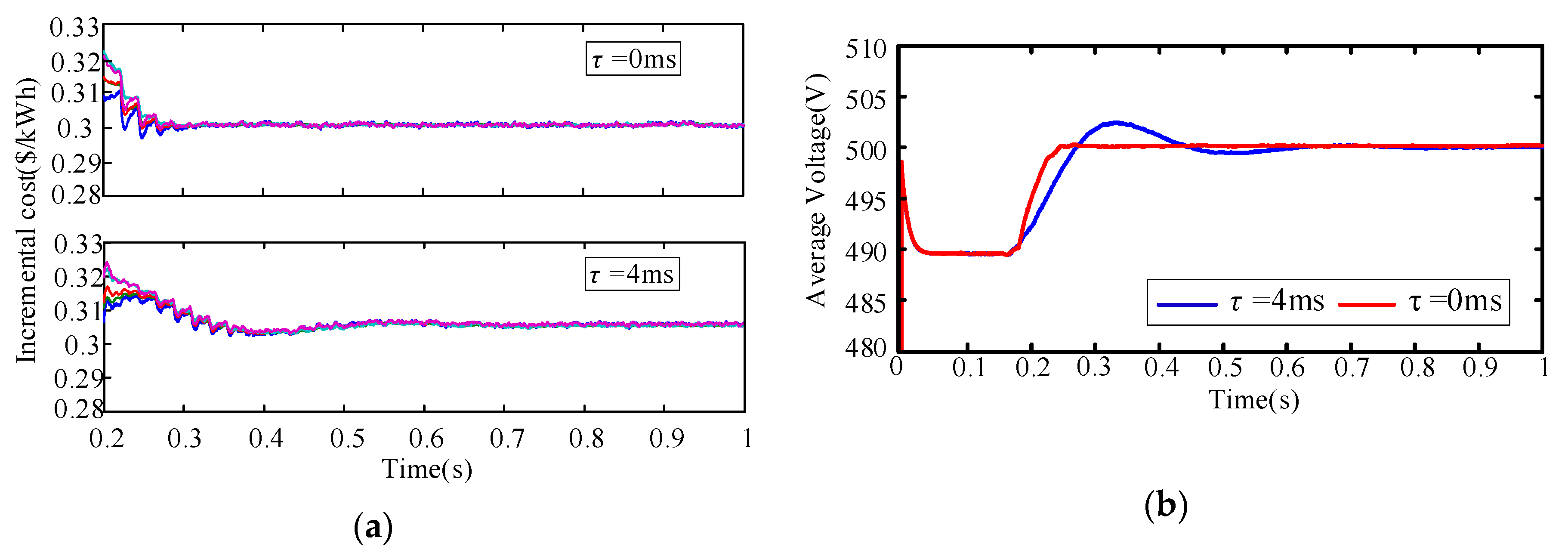
First, the performance of common topology is tested under different time delay. Initially, the total demand is 30 kW, and regulation process is enabled at 0.2 s. It can be seen from Figure 16 that the incremental costs and average voltage soon converge to the target values without any oscillation when τact = 0 s. However, when τact = 4 ms, the equal incremental costs and average voltage achieve their stable state through a large oscillation process. On the other hand, based on (39), when τact = 4 ms, the spectral radius of the common topology is calculated: esr(Ψ(2)) = 0.8497, the corresponding eigenvalue is −0.362 ± 0.769i. Thus, the reason for the oscillation process is that the large spectral radius leads to the voltage estimation unfinished under 11 iterations, which causes the voltage correction term in each voltage regulator different. Therefore, the voltage deviation among different converters results in power and voltage oscillation in turn, as shown in Figure 16a,b.
Similarly, the performance of optimal topology is also tested under different time delay. It can be seen from Figure 17 that the incremental costs and average voltage soon converge to the objective values without any oscillation when τact = 0 s. When τact = 4 ms, the equal incremental costs and average voltage achieve their stable state without much fluctuation. From the calculation of (39) under the optimal topology, the spectral radius of the optimal topology with the same τact is calculated: esr(Ψ(2)) = 0.7975, the corresponding eigenvalue is 0.526 ± 0.6i. The smaller spectral radius causes smaller voltage deviation among different converters. Thus, the voltage regulation and economical regulation time are less than that of the common one, and the maximum overshoot of the oscillation are smaller as well.
Thus, it can be concluded that the performance of both topologies will decrease when time delay occurs. However, the spectral radius of the optimal topology is smaller than that of the common topology at the same time delay, therefore the regulation speed under optimal topology is faster. In other words, the optimal topology has a better effect in inhibiting oscillation. It is noting that the optimal ring topology is selected based on the same weight (ξ1 = ξ2 = 0.5). If the construction cost is neglected, then the weight should be: ξ1 = 1, ξ2 = 0, and the corresponding optimal topology will also change.
6. Conclusions
A distributed economical dispatch scheme containing three control levels is proposed in this paper for the droop-based autonomous DC microgrid. It can be seen from the simulation results that the proposed scheme can achieve the control target effectively without degrading the stability of the system. Moreover, the comparison in the primary level and secondary level show that the proposed droop control has a better dynamic response, and the distributed voltage regulation scheme can recover the average voltage of the system smoothly without voltage and power oscillation. The comparison in the tertiary level illustrates that the proposed economical regulation can achieve the global optimum without the centralized controller, and the accuracy of the optimum is verified by the mathematical programming method. Furthermore, the capability of plug and play of the proposed scheme ensures the convergence performance of the system and meets the flexible operation requirement. Finally, the performance of inhibiting oscillation of the optimal topology is verified under different time delays.
Author Contributions
Methodology, X.D.; validation, M.Z. and W.H.; writing—original draft, Z.L.; writing—review and editing, Z.W. All authors have read and agreed to the published version of the manuscript.
Funding
This research was funded by Open Foundation of Jiangsu Key Laboratory of Smart Grid Technology and Equipment and the National Key R&D Program of China (2016YFB0900500).
Conflicts of Interest
The authors declare no conflict of interest.
References
- Lasseter, R.H. Smart distribution: Coupled microgrids. Proc. IEEE 2011, 99, 1074–1082. [Google Scholar] [CrossRef]
- Lou, G.; Gu, W.; Wang, W.; Song, X.; Gao, F. Distributed model predictive secondary voltage control of islanded microgrids with feedback linearization. IEEE Access 2018, 6, 50169–50178. [Google Scholar] [CrossRef]
- Anand, S.; Fernandes, B.G.; Guerrero, J. Distributed control to ensure proportional load sharing and improve voltage regulation in low-voltage dc microgrids. IEEE Trans. Power Electron. 2013, 28, 1900–1913. [Google Scholar] [CrossRef] [Green Version]
- Wang, P.; Lu, X.; Yang, X.; Wang, W.; Xu, D. An improved distributed secondary control method for dc microgrids with enhanced dynamic current sharing performance. IEEE Trans. Power Electron. 2016, 31, 6658–6673. [Google Scholar] [CrossRef]
- Nutkani, I.U.; Loh, P.C.; Blaabjerg, F. Droop scheme with consideration of operating costs. IEEE Trans. Power Electron. 2014, 29, 1047–1052. [Google Scholar] [CrossRef]
- Abido, M.A. Optimal design of power-system stabilizers using particle swarm optimization. IEEE Trans. Energy Convers. 2002, 17, 406–413. [Google Scholar] [CrossRef]
- Linda, M.M.; Nair, N.K. Optimal design of multi-machine power system stabilizer using robust ant colony optimization technique. IEEE Trans. Instrum. Meas. Control 2012, 34, 829–840. [Google Scholar] [CrossRef]
- Meng, L.; Dragicevic, T.; Guerrero, J.M. Stability constrained efficiency optimization for droop-controlled DC-DC conversion system. In Proceedings of the 39th Annual Conference of the IEEE Industrial Electronics Society, Vienna, Austria, 10–13 November 2013; pp. 7222–7227. [Google Scholar]
- Yazdanian, M.; Mehrizi-Sani, A. Distributed control techniques in microgrids. IEEE Trans. Smart Grid 2014, 5, 2901–2909. [Google Scholar] [CrossRef]
- Nutkani, I.U.; Loh, P.C.; Wang, P.; Blaabjerg, F. Cost-prioritized droop schemes for autonomous ac microgrids. IEEE Trans. Power Electron. 2015, 30, 1109–1119. [Google Scholar] [CrossRef]
- Nutkani, I.U.; Wang, P.; Loh, P.C.; Blaabjerg, F. Autonomous economic operation of grid connected DC microgrid. In Proceedings of the IEEE 5th International Symposium on PEDG, Galway, Ireland, 24–27 June 2014; pp. 1–5. [Google Scholar]
- Nutkani, I.U.; Wang, P.; Loh, P.C.; Blaabjerg, F. Cost-based droop scheme for DC microgrid. In Proceedings of the 2014 IEEE Energy Conversion Congress and Exposition (ECCE), Pittsburgh, PA, USA, 14–18 September 2014; pp. 765–769. [Google Scholar]
- Xin, H.; Zhao, R.; Zhang, L.; Wang, Z.; Wong, K.P.; Wei, W. A decentralized hierarchical control structure and self-optimizing control strategy for F-P type DGs in islanded microgrids. IEEE Trans. Smart Grid 2016, 7, 3–5. [Google Scholar] [CrossRef]
- Chen, F.; Chen, M.; Li, Q.; Meng, K.; Zheng, Y.; Guerrero, J. Cost-based droop schemes for economic dispatch in islanded microgrids. IEEE Trans. Smart Grid 2017, 8, 63–74. [Google Scholar] [CrossRef] [Green Version]
- Nutkani, I.U.; Loh, P.C.; Wang, P.; Blaabjerg, F. Linear decentralized power sharing schemes for economic operation of AC microgrids. IEEE Trans. Ind. Electron. 2016, 63, 225–234. [Google Scholar] [CrossRef]
- Xu, Y.; Liu, W. Novel Multiagent Based Load Restoration Algorithm for Microgrids. IEEE Trans. Smart Grid 2011, 2, 152–161. [Google Scholar] [CrossRef]
- Li, P.; Zhang, C.; Wu, Z.; Xu, Y.; Hu, M.; Dong, Z. Distributed adaptive robust voltage/var control with network partition in active distribution networks. IEEE Trans. Smart Grid 2019, in press. [Google Scholar] [CrossRef]
- Nasirian, V.; Moayedi, S.; Davoudi, A.; Lewis, F.L. Distributed cooperative control of dc microgrids. IEEE Trans. Power Electron. 2015, 30, 2288–2303. [Google Scholar] [CrossRef]
- Nasirian, V.; Davoudi, A.; Lewis, F.L.; Guerrero, J.M. Distributed adaptive droop control for DC distribution systems. IEEE Trans. Energy Convers. 2014, 29, 944–956. [Google Scholar] [CrossRef] [Green Version]
- Xu, Y.; Zhang, W.; Liu, W. Distributed dynamic programming-based approach for economic dispatch in smart grids. IEEE Trans. Ind. Inform. 2015, 11, 166–175. [Google Scholar] [CrossRef]
- Wang, Z.; Wu, W.; Zhang, B. A fully distributed power dispatch method for fast frequency recovery and minimal generation cost in autonomous microgrids. IEEE Trans. Smart Grid 2016, 7, 19–31. [Google Scholar] [CrossRef]
- Binetti, G.; Davoudi, A.; Naso, D.; Turchiano, B.; Lewis, F.L. A distributed auction-based algorithm for the nonconvex economic dispatch problem. IEEE Trans. Ind. Inform. 2014, 10, 1124–1132. [Google Scholar] [CrossRef]
- Zhang, Z.; Chow, M.Y. Convergence analysis of the incremental cost consensus algorithm under different communication network topologies in a smart grid. IEEE Trans. Power Syst. 2012, 27, 1761–1768. [Google Scholar] [CrossRef]
- Zhang, W.; Xu, Y.; Liu, W.; Zhang, C.; Yu, H. Distributed online optimal energy management for smart grids. IEEE Trans. Ind. Inform. 2015, 11, 717–727. [Google Scholar] [CrossRef]
- Xu, Y.; Zhang, W.; Hug, G.; Kar, S.; Li, Z. Cooperative control of distributed energy storage system in a microgrid. IEEE Trans. Smart Grid 2015, 6, 238–248. [Google Scholar] [CrossRef]
- Xu, Y.; Li, Z. Distributed optimal resource management based on the consensus algorithm in a microgrid. IEEE Trans. Ind. Electron. 2015, 62, 2584–2592. [Google Scholar] [CrossRef]
- Rahbari-Asr, N.; Ojha, U.; Zhang, Z.; Chow, M.Y. Incremental welfare consensus algorithm for cooperative distributed generation/demand response in smart grid. IEEE Trans. Smart Grid 2014, 5, 2836–2845. [Google Scholar] [CrossRef]
- Hu, J.; Duan, J.; Ma, H.; Chow, M.Y. Distributed adaptive droop control for optimal power dispatch in dc microgrid. IEEE Trans. Ind. Electron. 2018, 65, 778–789. [Google Scholar] [CrossRef]
- Moayedi, S.; Davoudi, A. Unifying distributed dynamic optimization and control of islanded DC microgrids. IEEE Trans. Power Electron. 2017, 32, 2329–2346. [Google Scholar] [CrossRef]
- Das, D.B.; Patvardhan, C. New multi-objective stochastic search technique for economic load dispatch. IEE Proc. Gener. Transm. Distrib. 1998, 145, 747–752. [Google Scholar] [CrossRef]
- Olfati-Saber, R.; Fax, J.A.; Murray, R.M. Consensus and cooperation in networked multi-agent systems. Proc. IEEE 2007, 95, 215–233. [Google Scholar] [CrossRef]
- Xiao, F.; Wang, L.; Wang, A. Consensus problems in discrete-time multiagent systems with fixed topology. J. Math. Anal. Appl. 2006, 322, 587–598. [Google Scholar] [CrossRef] [Green Version]
- Franklin, G.F.; Workman, M.L.; Powell, D. Digital Control of Dynamic System, 2rd ed.; Addison-Wesley Longman Publishing Co., Inc.: Boston, MA, USA, 1990. [Google Scholar]
- Wang, L.; Xiao, F. A new approach to consensus problems in discrete-time multiagent systems with time-delays. Sci. China Ser. F Inf. Sci. 2007, 50, 625–635. [Google Scholar] [CrossRef]
- Braitor, A.; Mills, A.R.; Kadirkamanathan, V.; Konstantopoulos, G.C.; Norman, P.G.; Jones, C.E. Control of DC power distribution system of a hybrid electric aircraft with inherent overcurrent protection. In Proceedings of the 2018 IEEE International Conference on Electrical Systems for Aircraft, Railway, Ship Propulsion and Road Vehicles & International Transportation Electrification Conference, Nottingham, UK, 7–9 November 2018; pp. 1–6. [Google Scholar]
- Cupelli, L.; Schumacher, M.; Monti, A.; Mueller, D.; De Tommasi, L.; Kouramas, K. Simulation Tools and Optimization Algorithms for Efficient Energy Management in Neighborhoods. In Energy Positive Neighborhoods and Smart Energy Districts; Elsevier: Amsterdam, The Netherlands, 2017; pp. 57–100. [Google Scholar]
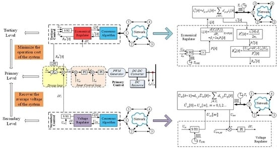
Figure 1.
Hierarchical distributed control for the converters.
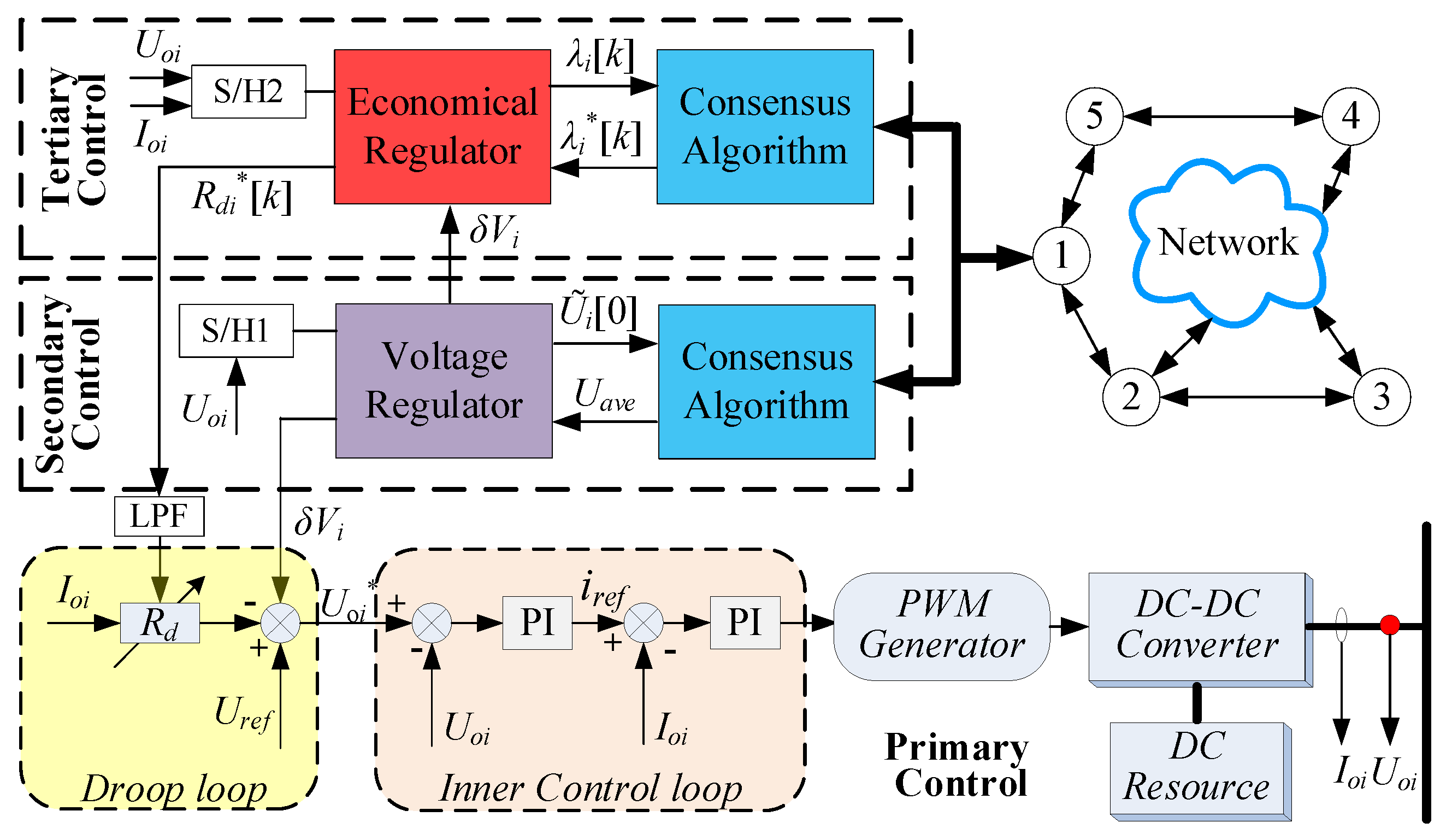
Figure 2.
Voltage regulation in secondary control level.
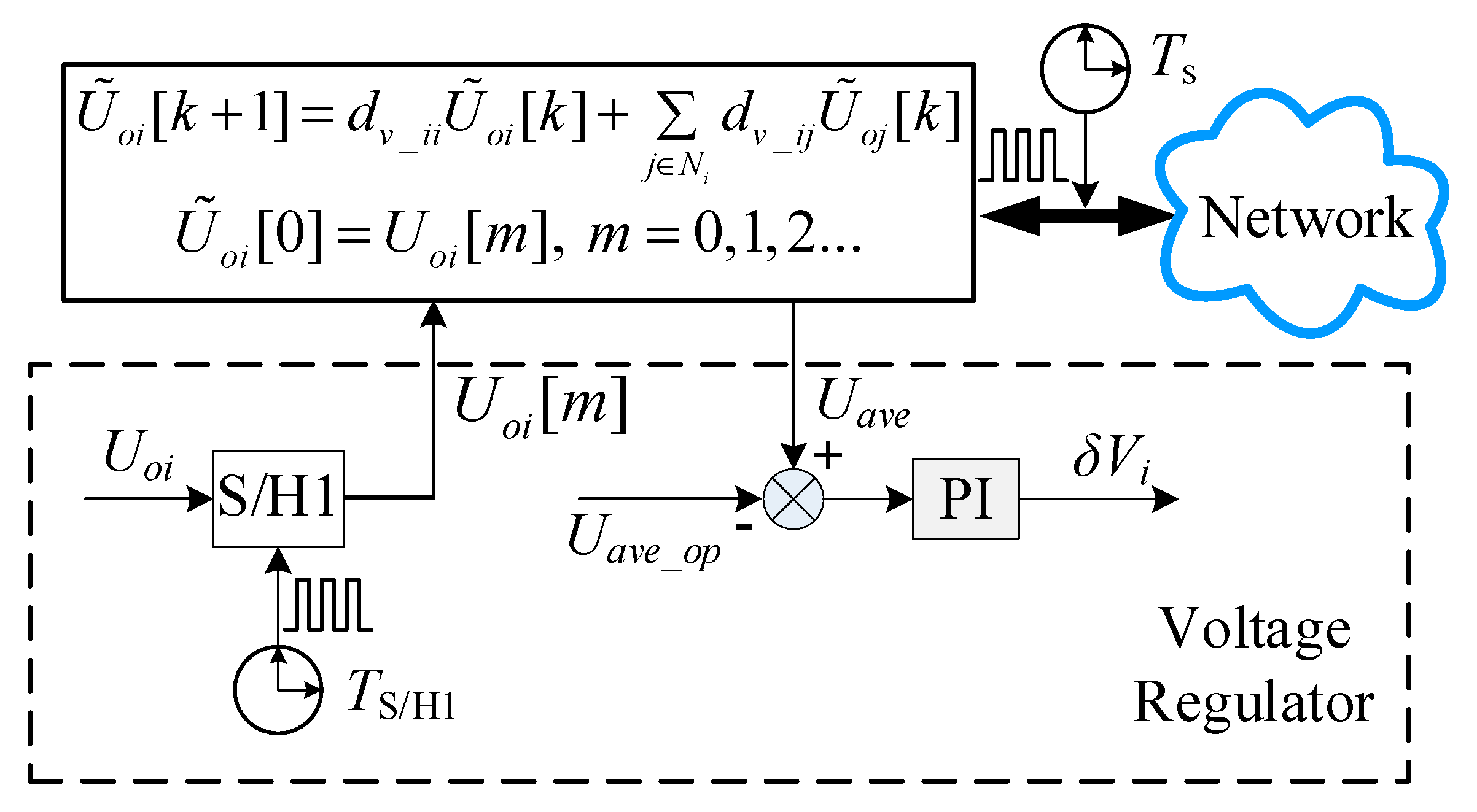
Figure 3.
Economical regulator in tertiary control level.

Figure 4.
Distribution of eigenvalues with different time delay.
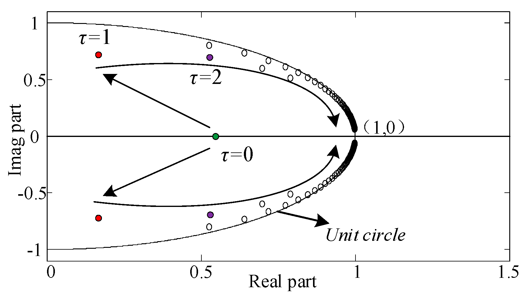
Figure 5.
Simulation system for direct current (DC) microgrid.
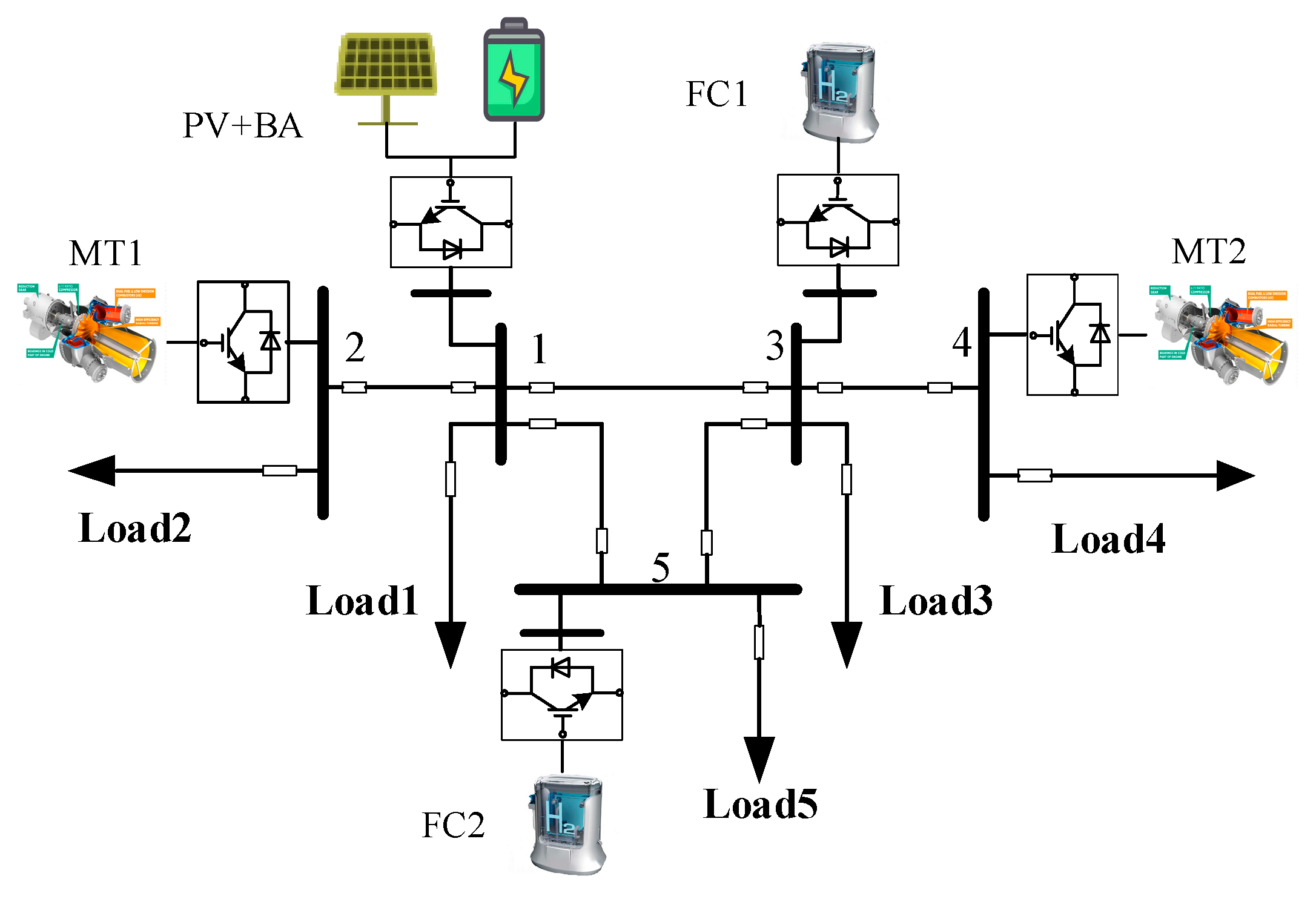
Figure 6.
Pareto frontier of the multi-objective optimization model.
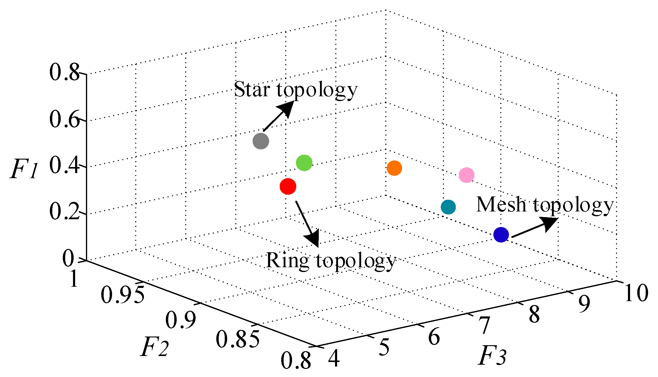
Figure 7.
Optimal topology and the corresponding matrix D. (a) the optimal topology; (b) the corresponding matrix.
Figure 7.
Optimal topology and the corresponding matrix D. (a) the optimal topology; (b) the corresponding matrix.
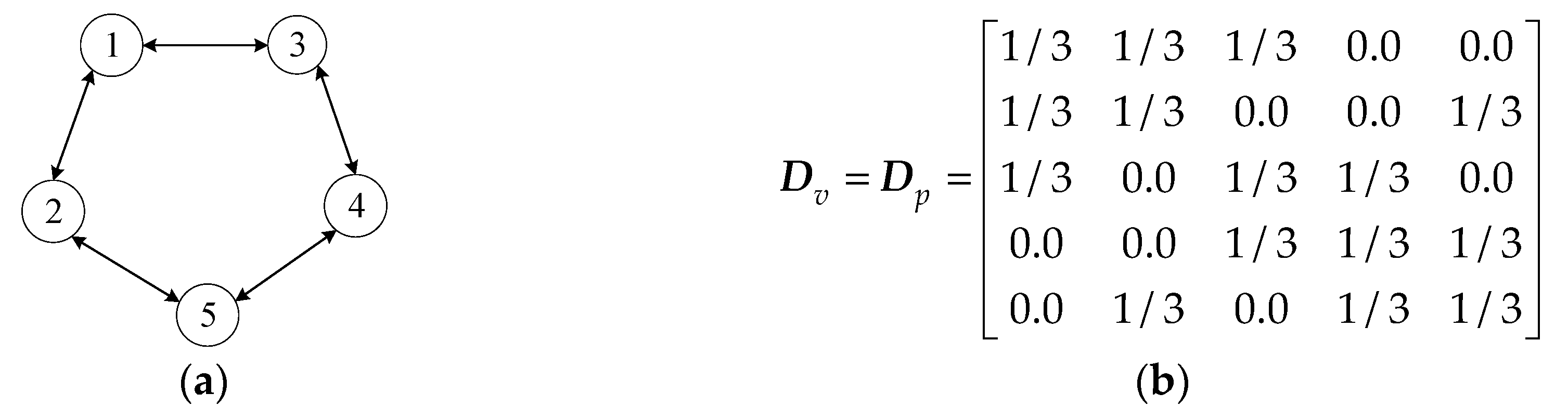
Figure 8.
Effect of the proposed scheme under changing load. (a) the output power of each generator; (b) the incremental cost of each generator; (c) the virtual resistance in each economical regulator; (d) the estimated voltage in each voltage regulator; (e) the bus voltages; (f) the average voltage of the system.
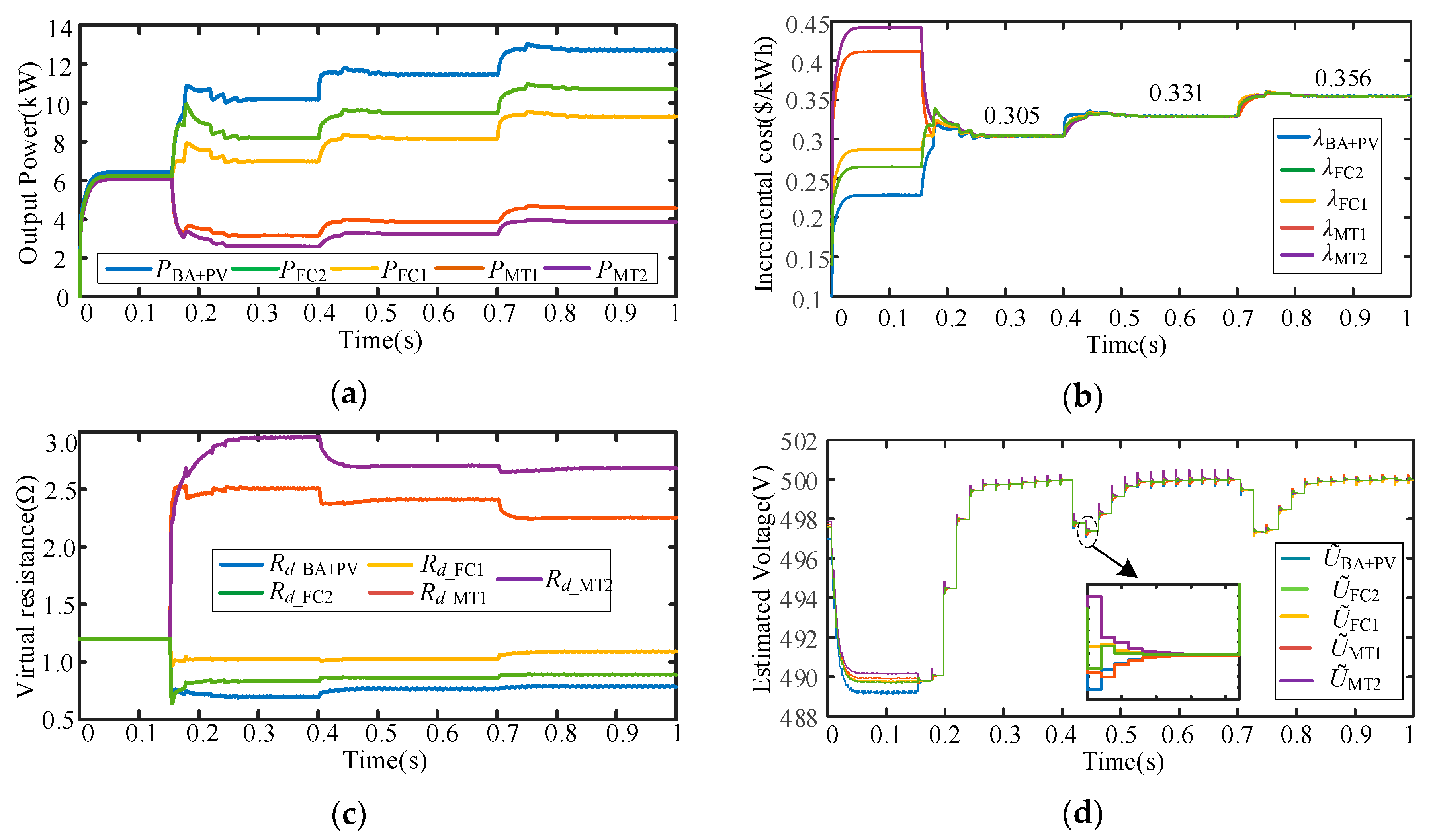
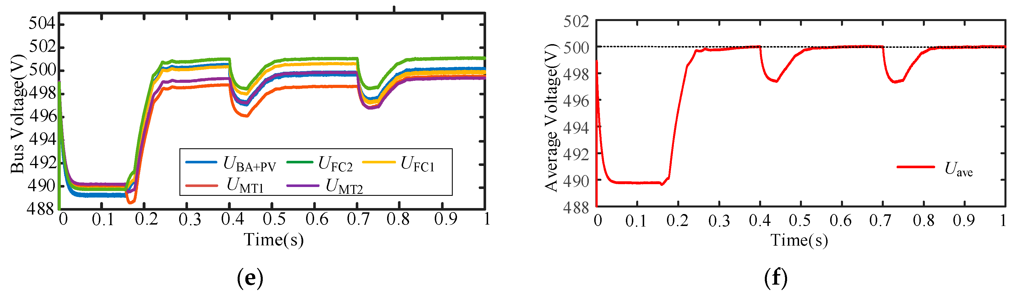
Figure 9.
The comparison between the proposed droop control and the one in [35]. (a) the output power of each generator based on the proposed scheme; (b) the bus voltages based on the proposed scheme; (c) the output power of each generator based on the one in [35]; (d) the bus voltages based on the one in [35].
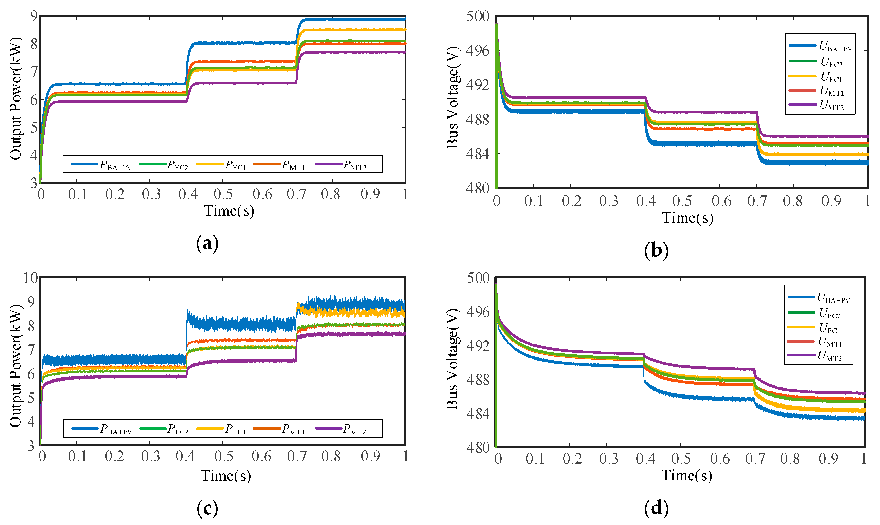
Figure 10.
The comparison between the proposed distributed control and the decentralized control in secondary level. (a) the output power of each generator based on the proposed scheme; (b) the bus voltages based on the proposed scheme; (c) the output power of each generator based on the decentralized scheme; (d) the bus voltages based on the decentralized scheme.
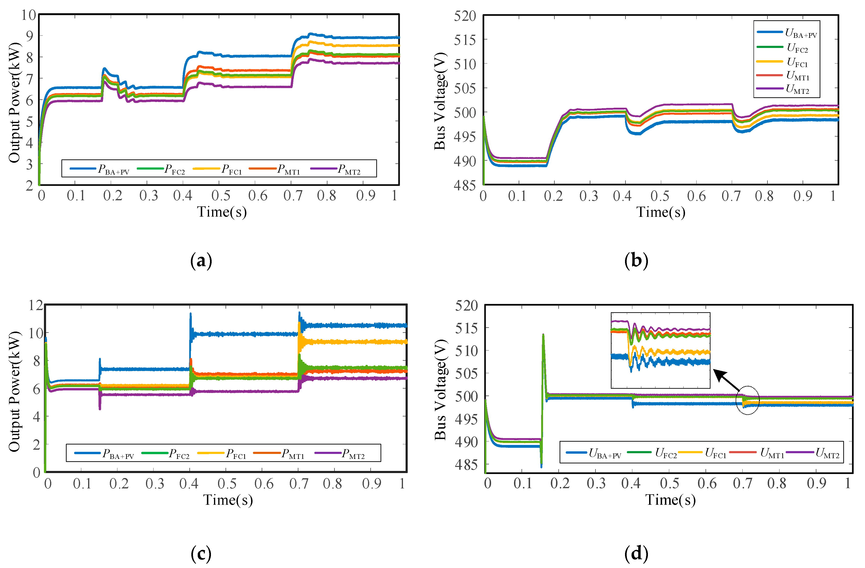
Figure 11.
The comparison between the proposed distributed control and the decentralized control in tertiary level. (a) the output power of each generator based on the proposed scheme; (b) the incremental costs based on the proposed scheme; (c) the output power of each generator based on the non-linear scheme; (d) the incremental costs based on the non-linear scheme.
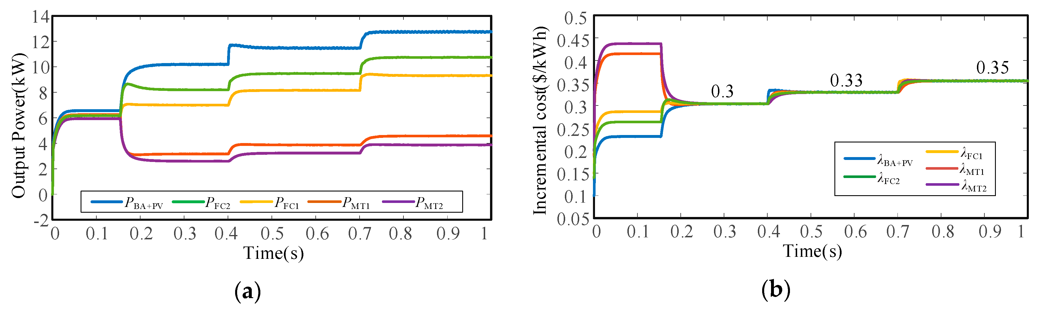
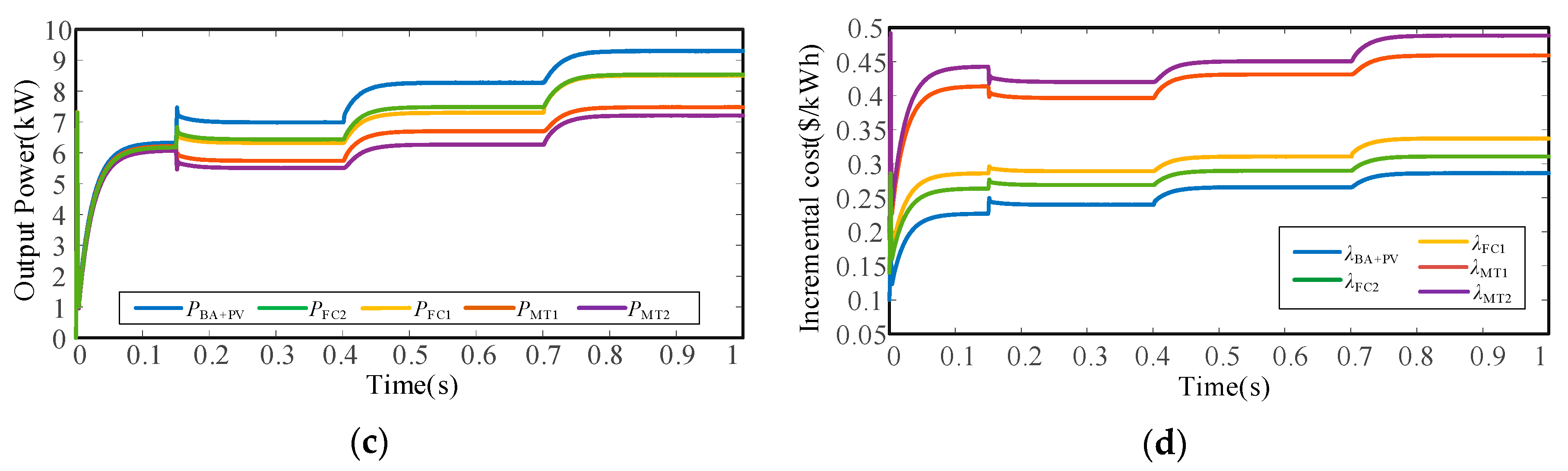
Figure 12.
Effect of the proposed scheme considering power limitation. (a) the total load demand; (b) the output power of each generator; (c) the incremental cost of each generator; (d) the bus voltages; (e) the average voltage of the system.
Figure 12.
Effect of the proposed scheme considering power limitation. (a) the total load demand; (b) the output power of each generator; (c) the incremental cost of each generator; (d) the bus voltages; (e) the average voltage of the system.
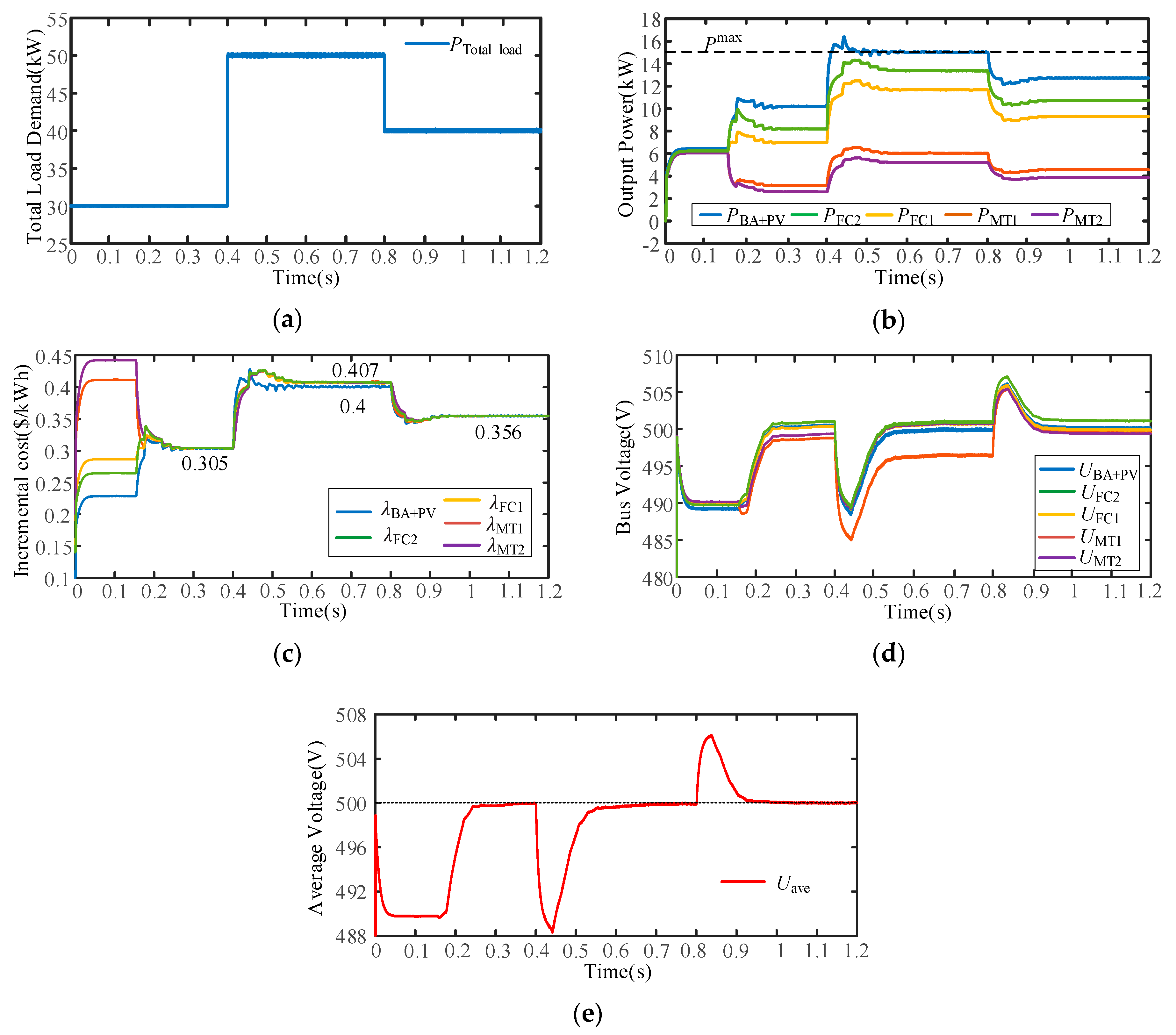
Figure 13.
The remaining topology and the corresponding matrix D^. (a) the remaining topology; (b) the corresponding matrix.
Figure 13.
The remaining topology and the corresponding matrix D^. (a) the remaining topology; (b) the corresponding matrix.

Figure 14.
Plug and play performance of the proposed scheme. (a) the output power of each generator; (b) the incremental cost of each generator; (c) the estimated voltage in each voltage regulator; (d) the bus voltages; (e) the average voltage of the system.
Figure 14.
Plug and play performance of the proposed scheme. (a) the output power of each generator; (b) the incremental cost of each generator; (c) the estimated voltage in each voltage regulator; (d) the bus voltages; (e) the average voltage of the system.
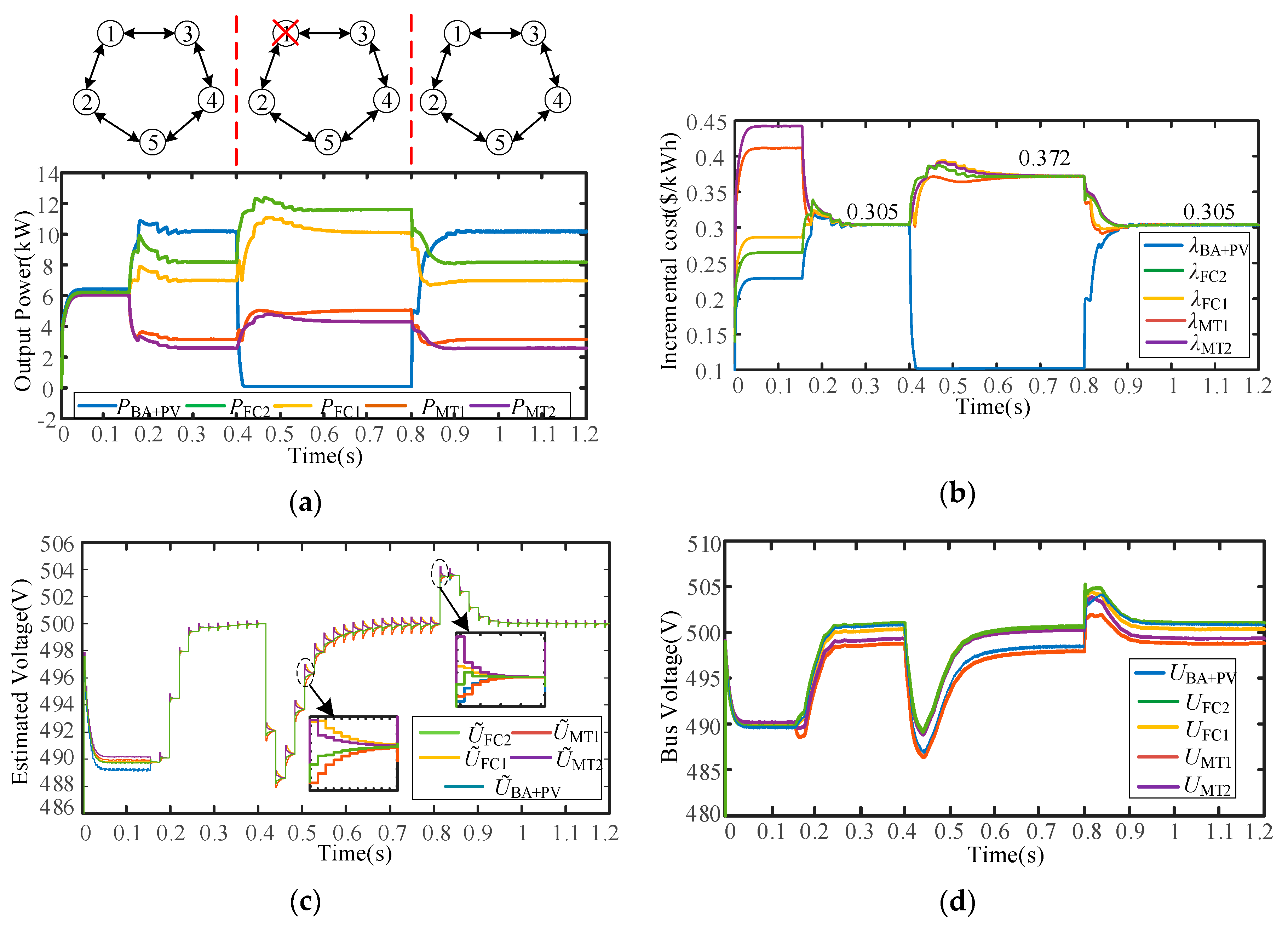

Figure 15.
Common topology and the corresponding matrix Dc. (a) the common topology; (b) the corresponding matrix.
Figure 15.
Common topology and the corresponding matrix Dc. (a) the common topology; (b) the corresponding matrix.
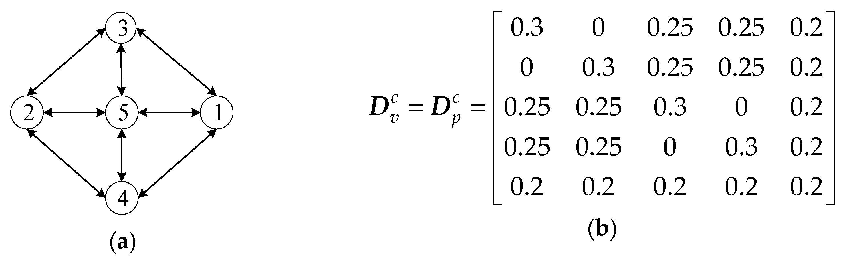
Figure 16.
Performance of the common topology. (a) the incremental costs under different delays; (b) the average voltages under different delays.
Figure 16.
Performance of the common topology. (a) the incremental costs under different delays; (b) the average voltages under different delays.
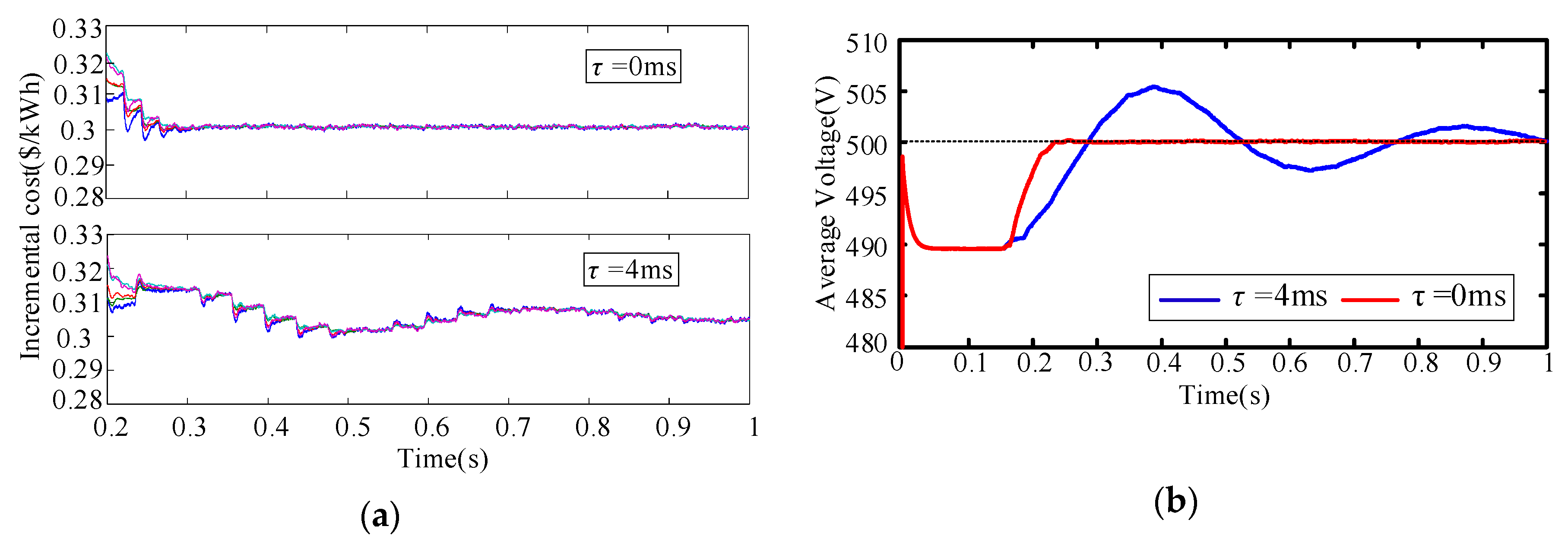
Figure 17.
Performance of the optimal topology. (a) the incremental costs under different delays; (b) the average voltages under different delays.
Figure 17.
Performance of the optimal topology. (a) the incremental costs under different delays; (b) the average voltages under different delays.

Table 1.
Cost function parameters of DGs.
| System | α ($/kW2h) | β ($/kWh) | γ ($/h) |
|---|---|---|---|
| PV + BA | 0.01 | 0.1 | 0.0015 |
| MT1 | 0.018 | 0.19 | 0.05 |
| FC1 | 0.011 | 0.15 | 0.015 |
| MT2 | 0.02 | 0.2 | 0.04 |
| FC2 | 0.01 | 0.14 | 0.01 |
Table 2.
Parameters of primary level.
| Parameters | Unit | Values |
|---|---|---|
| Nominal dc voltage | V | 500 |
| System reference voltage | V | 505 |
| Filter inductance | mH | 5 |
| DC capacitance | uF | 1600 |
| Initial virtual resistance | Ω | 1.2 |
| Switch frequency | kHz | 10 |
| Load 2, 3, 4, 5 | kW | 5 |
| Load 1 | kW | 10 |
| Line resistance | Ω | 0.4 |
| Maximum output | kW | 15 |
Table 3.
Parameters of voltage and economical regulator.
| kp | ki | N | Ts (ms) | Tm (ms) | Uave_op (V) |
|---|---|---|---|---|---|
| 0.3 | 15 | 11 | 2 | 6 | 500 |
Table 4.
The comparison between the mathematical programming and the proposed scheme.
| Parameters | Mathematical Programming | The Proposed Scheme | ||||
|---|---|---|---|---|---|---|
| 0.15–0.4 s | 0.4–0.7 s | 0.7–1 s | 0.15–0.4 s | 0.4–0.7 s | 0.7–1 s | |
| P1 (kW) | 10.0 | 11.29 | 12.45 | 10.20 | 11.50 | 12.75 |
| P2 (kW) | 3.10 | 3.82 | 4.42 | 3.16 | 3.87 | 4.58 |
| P3 (kW) | 6.83 | 8.0 | 9.05 | 7.0 | 8.15 | 9.32 |
| P4 (kW) | 2.55 | 3.2 | 3.73 | 2.60 | 3.23 | 3.88 |
| P5 (kW) | 8.0 | 9.3 | 10.45 | 8.18 | 9.45 | 10.74 |
| Uo1 (V) | 501.1 | 500.7 | 501.5 | 500.5 | 499.4 | 500.0 |
| Uo2 (V) | 496.4 | 496.5 | 498.1 | 498.80 | 498.2 | 499.4 |
| Uo3 (V) | 500.9 | 502.3 | 501.3 | 500.25 | 500.91 | 499.5 |
| Uo4 (V) | 498.9 | 500.84 | 500.0 | 498.20 | 499.41 | 498.5 |
| Uo5 (V) | 502.5 | 503.6 | 503.9 | 501.9 | 502.2 | 502.5 |
© 2020 by the authors. Licensee MDPI, Basel, Switzerland. This article is an open access article distributed under the terms and conditions of the Creative Commons Attribution (CC BY) license (http://creativecommons.org/licenses/by/4.0/).
Share and Cite
MDPI and ACS Style
Lv, Z.; Wu, Z.; Dou, X.; Zhou, M.; Hu, W. Distributed Economic Dispatch Scheme for Droop-Based Autonomous DC Microgrid. Energies 2020, 13, 404. https://doi.org/10.3390/en13020404
AMA Style
Lv Z, Wu Z, Dou X, Zhou M, Hu W. Distributed Economic Dispatch Scheme for Droop-Based Autonomous DC Microgrid. Energies. 2020; 13(2):404. https://doi.org/10.3390/en13020404
Chicago/Turabian StyleLv, Zhenyu, Zaijun Wu, Xiaobo Dou, Min Zhou, and Wenqiang Hu. 2020. "Distributed Economic Dispatch Scheme for Droop-Based Autonomous DC Microgrid" Energies 13, no. 2: 404. https://doi.org/10.3390/en13020404
Note that from the first issue of 2016, this journal uses article numbers instead of page numbers. See further details here.