Quantifying the Demand Response Potential of Inherent Energy Storages in Production Systems

Abstract

The increasing share of volatile, renewable energy sources rises the demand for consumers who can shift their electrical power demand in time. In theory, the industrial sector offers great potential here, as it accounts for a large proportion of electricity demand. However, the heterogeneous structure of facilities in factories and the concerns of operators regarding data security and process control often prevent the implementation of demand side management measures in this sector. In order to counteract these obstacles, this paper presents a general mathematical framework for modelling and evaluating different types of inherent energy storages (IES) which typically can be found in industrial production systems. The method can be used to calculate the flexibility potential of the IES in a factory with focus on hysteresis-controlled devices and make the potential visible and usable for power grid stabilization. The method is applied in a typical production line from metalworking industry to provide live monitoring of the current flexibility potential of selected devices.

1. Introduction

The energy system in Germany and many other countries of the world is currently in a state of transition. In the past, electricity systems were centrally managed with conventional base load-capable power plants only. These generated electricity at high voltage level according to the consumer’s requirements. Renewable power plants instead often feed in decentral at lower voltage levels and their generation capacities depend on the seasons and daily changing weather. The increasing usage of regenerative energy sources in Germany requires a comprehensive system redesign [1,2]. In order to maintain future grid stability at acceptable costs it will be necessary for more consumers to shift their electric loads in time [3,4]. Especially the industrial sector can make a large contribution to demand response (DR), as it accounts for 45.7% of Germanys electricity demand [5].

The active participation of industrial consumers to DR requires knowledge of the actual flexibility of the electrical power demand. However the current electricity market design has few incentives especially for smaller organizations to motivate the companies for providing systemically useful load management measures [6,7]. There are currently various efforts to change this, as shown, for example, by the activities to transform the European electricity market. These explicitly take into account the simplification of market access for flexible electricity consumers, but the transformation process is not yet complete [8]. In addition, factories have a highly heterogeneous plant structure due to their specialization on different industry branches. This leads to the fact that many companies do not have precise knowledge of the existing flexibility potential in their processes and therefore cannot participate in DR. However, the heterogeneity of machines and devices in industrial processes is only at first glance an obstacle for flexible electrical energy demand. A closer analysis often reveals that many processes are very similar in the mathematical characteristics which define their flexibility potential. There are different approaches to group flexibilities into categories in order to make solutions that have been developed for a specific plant transferable to other plants [3,9,10,11]. For example, in [10] flexible load is distinguished into three categories—“Buckets”, which can be described as energy storages with defined capacity limits, “Batteries” which have the additional restriction that they must be fully charged at a certain time and “Bakeries”, where the device that charges the energy storage must remain switched on for a defined time span.

Based on these considerations, this paper analyzes inherent energy storages (IES). IES are another category of energy storage-like flexibilities that are very common in industrial processes. Examples for IES in production systems are electrical heated tanks of a cleaning machine, the cooling system of a machine tool or the air-conditioning system of a production hall. They all have inherent storage capacities that make it possible to decouple the devices’ electricity consumption from the use of the form of energy required. According to [12] IES are using the tolerances of different state variables in a process to store energy. The additional restriction in making the operation of these devices more flexible is that the useful energy demand of the production process must always be covered. This paper presents a mathematical model to calculate the flexibility potential of inherent energy storages with classical key indicators known from the energy markets. Furthermore, a method is presented how the flexibility potential of the devices can be extracted from measured data of the electrical energy demand or state variables.

The paper is structured as follows: first an overview of current research in the field of industrial demand response and the use of inherent energy storages in other sectors is given. Afterwards the developed modelling method for IES is described in Section 2. Using examples, the energetic formulas to describe IES are developed and the basics for the calculation of an IES’ flexibility potential are explained. It is shown how to calculate the reference load profile and different flexible load profiles depending on the method by which the flexibility measure is activated. In Section 3 the developed method is applied in a case study on two machines in the ETA research factory of the Technical University of Darmstadt, where data from a typical metalworking production line can be used for testing the method regarding its practical applicability. The last chapter discusses the results and gives an outlook to further research.

Related Work

Current research on DR in the industrial sector is focused on specific high energy consuming processes for example paper production [13], steel plants [14,15], chemical industry [16] or cement plants [17,18]. The industrial sectors of paper production, basic chemicals, metal production and stone and earth processing together account for 65% of the energy demand in Germany. An analysis of these sectors therefore covers in principle a large share of the energy demand [19]. However, the analyses are usually process-specific and not easily transferable to other industries. An overview of current research activities, especially in the area of potential analysis of the industrial sector as a whole, is provided for example by [20] and [21].

In contrast to the lack of transferrable approaches in the industrial sector, methods and technical solutions to qualify inherent storage capacities for DR in the private sector is a much-debated research field. Especially using the thermal inertia of thermostatically controlled loads (TCLs) like refrigerators or electrical boilers is often discussed and analysed mathematically: In Conte et al. a simulation shows how the coordinated control of refrigerators in combination with water heating systems can compensate the frequency fall-off after the blackout of a large-scale power plant in Sardinia [22]. In [23] the authors are using three different approaches to control a pooled system containing 900,000 individual fridges and freezers. The data was based on estimations for households in Canada. In [24] an algorithm is presented to optimize a large amount of thermostatically controlled devices in household by communicating through a central instance and thereby aggregating the devices to a distributed virtual energy storage system. Furthermore the usage of heating, ventilation and air conditioning (HVAC) systems of buildings for DR is often mentioned in literature: In [25] the usage of 1000 air handling units as primary operating reserve and their benefit to the power grid stability is simulated. The authors in [26] investigate the extent to which concrete core activation can increase the inherent energy storage capacity of different building types and how it can be used for electrical load transfer. In [27] the flexibility potential of inherent energy storages, called “non electrical energy storages”, is analyzed in private households. These considerations are also transferable to industrial processes.

The approaches from the private sector to retrieve the flexibility potential of IES and especially hysteresis controlled systems can be divided into two main categories: direct load control (DLC) on the one hand, where the device is switched remotely by the instance requesting the flexibility. On the other hand, there are approaches in which the hysteresis limits of the devices are adapted to a certain signal [23]. Studies from this field show, that if controlled by a central instance a large pool of thermostatically controlled loads can follow any desired load signal and thereby can participate in DR just as well as optimized high energy consuming processes [28].

The aim of this paper is to close the gap between research activities in the industrial and private sector in order to make the inherent storage capacities of different production processes usable for the electricity grid. The presented methods provide a general framework for the evaluation of the flexibility potential of IES in production systems, in particular with focus on hysteresis-controlled devices.

2. Modelling of IES

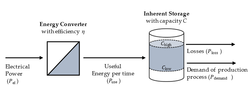
Inherent energy storages consist of a storage capacity and an energy converter which converts electrical energy into the desired energy form or the type of energy carrier that is required by the production process. Examples for required energy forms are thermal energy in heating and cooling processes or mechanical energy of conveyor systems, which remove waste materials from production machines. Typical energy carriers are compressed air in pneumatic supply systems, fluids in hydraulic systems or the airflow in ventilation and exhaust air systems. The amount of energy or energy carrier which is provided by the energy converter to the production process per time, is referred to as $P_{\mathrm{use}}$ in the following. The concept of inherent energy storages in production systems was introduced in [12] and defined as the “usage of tolerances of different state variables in processes as energy storage”. This illustrates the goal that is common to all inherent energy storages: keeping a certain value within defined limits, e.g., the temperature of a cooling system or the pressure in a compressed air supply system. The greater the range between the upper and lower limit, the more flexible is the system to shift its electrical energy consumption in time. This flexibility can be used to shift electrical loads, similar to an electrical energy storage system. To calculate the hereby generated equivalent electrical energy content $E$, models are needed to describe the characteristics of the different types of inherent storage systems. Against the background, we propose a general substitute model for IES shown in Figure 1. The basic key indicators included in this model are

• $P_{\mathrm{el}}:$electrical power required by the energy converter,
• $\eta$: efficiency of the converter in the conversion of electricity into useful energy,
• $P_{\mathrm{use}}:$ generated useful energy per time,
• $C$: the theoretical storage capacity,
• $C_{\mathrm{high}}:$upper level of usable storage capacity (upper level of storage content),
• $C_{\mathrm{low}}:$lower level of usable storage capacity (lower level of storage content),
• $P_{\mathrm{losses}}:$losses per time,
• $P_{\mathrm{demand}}:$energy demand per time of the production process.

Physical modeling of all kind of inherent energy storages cannot be completely standardized. The more complex the production facilities and boundary conditions are, the more specific the models become in order to be able to represent all interrelationships exactly. Nevertheless, there is the possibility to establish simplified physical substitute models for inherent energy storages, which allow a comparison of different types of IES. This is especially helpful when evaluating complex factory systems in order to prioritize promising devices instead of spending a lot of time on the analysis of devices with low potentials.

2.1. Examples for IES in Production

The values which must be kept between the upper and lower level are indicators for the state of charge (SOC) of the inherent energy storage. In case of thermal energy for example, the SOC indicator is the temperature in the heated or cooled storage capacity. When the SOC indicator reaches the upper limit, the energy storage is fully charged, when it reaches the lower limit it is empty.

Table 1. Examples for inherent energy storages in production systems.

SOC Indicator	Example	Typical Converter with Typical Efficiency	Formula for Inherent Storage Capacity 1
Temperature ($T$)	Heated water tank	Heating element 100%	$V· \rho ·c_p·\left(T_{high}-T_{low}\right)$	[29]
Temperature ($T$)	Machine cooling	Compression chiller 350% 2	$V· \rho ·c_p·\left(T_{high}-T_{low}\right)$	[27]
Pressure ($p$)	Compressed air generation with buffer tank	Compressor 60% 3	$V ·p_{high}·ln\frac{p_{high}}{p_{low}}$	[27] 4
Concentration ($c$)	Ventilated hall with CO2-Sensor	Ventilation System 0.35–0.56 Wh/m3 5	$V · \left(c_{high}-c_{low}\right)$	[27]
Filling level ($c$)	Lifting pump in machine tool	Pump 55 Wh/m3 6	$V · \left(c_{high}-c_{low}\right)$	[27]

¹ with volume ($V$), density ($\rho$), specific heat capcity ($c_p$). ² typical value for coefficient of performance [30]. ³ including motor and compressor losses, no leakage or pressure losses in pipes considered [31]. ⁴ formula for isothermal compression and ideal gas. ⁵ minimum efficiency requirements for ventilation systems in non-residential buildings [32] ⁶ specific electrical power consumption of a machine tool’s lifting pump [33].

shows typical examples for inherent energy storages in production systems and the main formulas to estimate the magnitude of the respective storage capacity.

In case of an exemplary electrically heated water tank, which can be found for example in all water-based cleaning machines, with a volume $V$ of 1.000 L, the density $\rho$(1.000 kg/m³) and specific heat capacity $c_p$ (4.12 kJ/kgK) of water and a target temperature $T$ of 60–65 °C the calculation of useful energy content results in 5.72 kWh. Since the conversion efficiency of the heating element can be assumed to be 100%, the equivalent electrical energy storage capacity is 5.72 kWh for this example, too. Assuming a nominal electrical power of 10 kW for the heating element and losses and demand to be zero, the minimum time the converter needs to fill the energy storages is 5.72 kWh/10 kW = 34.3 min. Regarding a compressed air system with a volume $V_2$ of 1 m³ and a target pressure $p_2$ of 7 bar, the calculation of the useful energy content results in 0.38 kWh, if the ambient pressure $p_1$ of 1 bar is taken as reference point. As the conversion efficiency of compressed air generation systems is at around 60%, the equivalent electrical energy storage for this example is 0.38 kWh/0.6 = 0.63 kWh. Thus, the minimum time for filling the storage amounts to 0.63 kWh/10 kW = 3.8 min in case of a compressor with a nominal electrical power of 10 kW. This simple assessment indicates that the thermal inherent energy storage has a far greater electrical flexibility potential, than the compressed air system although the volume of the storage and the nominal electrical power of the energy converter are equal. In this calculation, however, the losses and the demand for useful energy from the production process have been neglected. In the following, we discuss how these values influence the actual flexibility potential of the devices. For this purpose, it is necessary to explain the most important mathematical interrelationships for describing the operation of inherent energy storages: Many IES are two-point, respectively hysteresis controlled. This means that the energy converter switches on ($s=1$), when the content in the storage reaches its lower limit which is defined by the operator. Afterwards, as long as the content is below the upper level, the converter remains in the switched-on state. Such devices can be modelled as a hybrid system consisting of discrete and continuous states [34]:

$$\frac{\mathrm{d}C}{\mathrm{d}t}=\{\begin{array}{cc} P_{\mathrm{use}}-P_{\mathrm{loss}}-P_{\mathrm{demand}}\hfill & \mathrm{if} \mathrm{energy} \mathrm{converter} \mathrm{is} \mathrm{ON} \left(s=1\right)\hfill \\ -P_{\mathrm{loss}}-P_{\mathrm{demand}}\hfill & \mathrm{if} \mathrm{energy} \mathrm{converte} \mathrm{is} \mathrm{OFF} \left(s=0\right)\hfill \end{array}$$

(1)

The electrical power $P_{\mathrm{el}}$ is calculated from $P_{\mathrm{use}}$ through:

$$P_{\mathrm{el}}=\frac{P_{\mathrm{use}}}{\eta }$$

(2)

Assuming that the efficiency is constant and thus the temporal decoupling between the coverage of demand and the purchase of electrical power has no influence on the efficiency, the discharge power $P_{\mathrm{discharge}}$, seen from the electrical grid, can be calculated by:

$$P_{\mathrm{discharge}}=\frac{P_{\mathrm{demand}}+P_{\mathrm{losses}}}{\eta }$$

(3)

Therefore, the change rate over time of the equivalent electrical energy content $E$ is defined by:

$$\frac{\mathrm{d}E}{\mathrm{d}t}=\{\begin{array}{cc}{P}_{\mathrm{el}}-P_{\mathrm{discharge}}& \mathrm{if} \mathrm{energy} \mathrm{converter} \mathrm{is} \mathrm{ON} \left(s=1\right)\\ -P_{\mathrm{discharge}}& \mathrm{if} \mathrm{energy} \mathrm{converte} \mathrm{is} \mathrm{OFF} \left(s=0\right)\end{array}$$

(4)

The maximum usable equivalent electrical energy content $E_{\max }$. of the storage unit is calculated from the difference between the upper and lower limits of the usable storage capacity divided by the efficiency:

$$E_{\max } =E_{\mathrm{high}}-E_{\mathrm{low}}=\frac{C_{\mathrm{high}}}{\eta }-\frac{C_{\mathrm{low}} }{ \eta }$$

(5)

These equations are needed to calculate the flexibility potential of a hysteresis-controlled system from the power grids’ point of view. The general procedure for this is derived in the following section.

2.2. General Remarks on the Calculation of the Flexibility Potential Calculation for IES

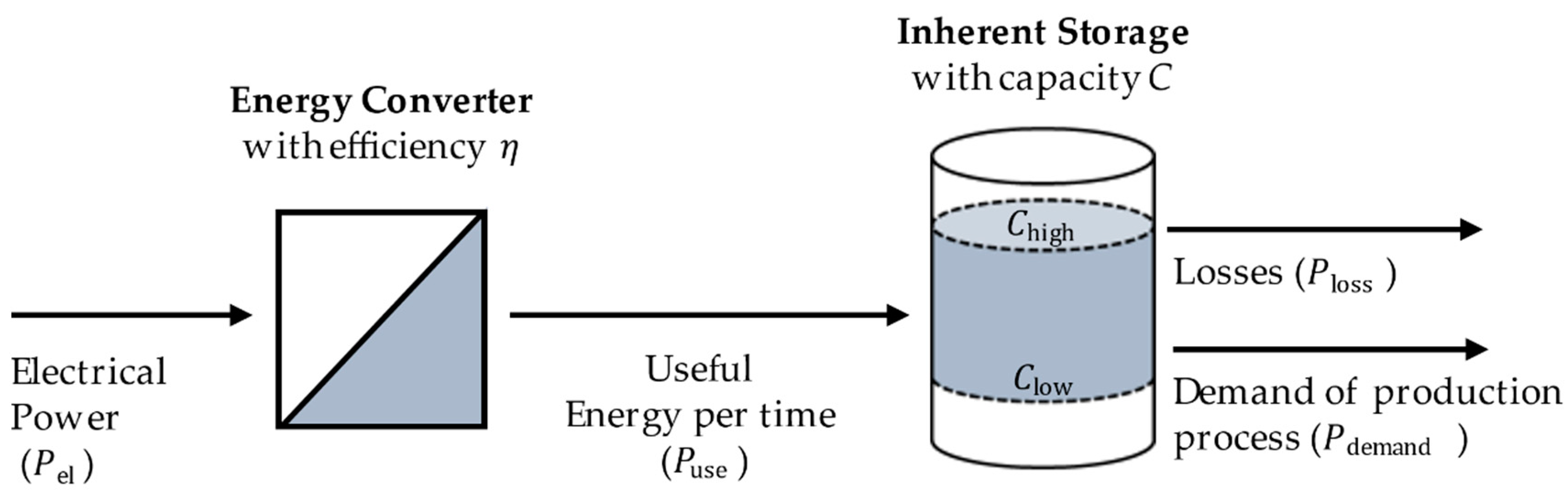
In general, the effectiveness of a load shifting measure for the power grid corresponds to the difference between the load profile in normal operation (reference load) and the load profile in energy flexible operation (flexible load) [12]. This is visualized in Figure 2 by the example of shifting the start of a defined electrical load from time step $t_0$ to $t_2$. By implementing the flexibility measure, a load change $\Delta P$ can be achieved and a defined amount of energy $E_{\mathrm{shift}}$ can be shifted in time.

The characteristics of the flexibility measure can be described by the following parameters which are based on the definition for standardized flexibility products which are for example discussed in [12,35]:

• $t_0$ to $t_1$: Activation time (from first load change to reach of final load level) $\Delta t_{\mathrm{activation}}$
• $t_1$ to $t_2$: Holding time (constant load level) $\Delta t_{\mathrm{hold}}$
• $t_2$ to $t_3$: Deactivation time (from load level to zero) $\Delta t_{\mathrm{deactivation}}$
• $t_3$ to $t_4$: Break time (time until load recovery starts) $\Delta t_{\mathrm{break}}$
• $t_3$ to $t_5$: Regeneration time (time until load recovery is completed) $\Delta t_{\mathrm{regeneration}}$

To quantify the flexibility potential of an inherent energy storage device, it is therefore necessary to know the reference load profile in order to compare it with the load profile in energy flexible operation mode. In the case of classic energy storages like batteries, but also cold and heat storage devices that are only used for the purpose of load shifting, the break and regeneration time are variable. This means that the operator is relatively unrestricted to decide when to catch up the load. The only limitations are standby losses of the storage unit. In case of IES, this statement no longer applies since there is a predefined demand load profile, which must be covered by the energy converter. In [36] the different types of energy storage are compared in terms of their suitability for demand response. The authors conclude that thermostatically controlled loads can be used for most system services of demand response if the necessary information and communication technology infrastructure is available.

2.3. Reference Load Profile

In order to simulate the operative behavior of a hysteresis controlled device, the following formulas can be used to calculate the electrical load profile and the energy content in each time step $t_{\mathrm{i}}$ of the time horizon which is considered. The formulas presuppose that the losses and the energy demand of the production process can be predicted and therefore $P_{\mathrm{discharge}}\left(t_i\right)$ is known for all time steps of the horizon. The timespan between $t_{\mathrm{i}}$ and $t_{\mathrm{i}-1}$ is called $\Delta t_{\mathrm{i}}$ in the following. In the first step, the storage’s energy content in case of maintaining the existing state of the energy converter is calculated:

$$\overline{E}\left(t_{\mathrm{i}}\right)=E\left(t_{\mathrm{i}-1}\right)+s\left(t_{\mathrm{i}-1}\right)\cdot P_{\mathrm{el},\mathrm{nom}}\cdot \Delta t_{\mathrm{i}}-P_{\mathrm{discharge}}\left(t_{\mathrm{i}}\right)\cdot \Delta t_{\mathrm{i}}$$

(6)

Hereby $P_{\mathrm{el},\mathrm{nom}}$ is the nominal electrical power of the energy converter, which is consumed if the converter is switched on. If the calculated value is between the upper and lower level of the energy storage capacity ($E_{\mathrm{low}}<\overline{E}\left(t_{\mathrm{i}}\right)<E_{\mathrm{high}}$), the state $s$ of energy converter can remain unchanged and the power can be calculated by:

$$P_{\mathrm{el}}\left(t_i\right)=\{\begin{array}{cc}{P}_{\mathrm{el},\mathrm{nom}}, & \mathrm{if} s\left(t_{\mathrm{i}-1}\right)=1\\ 0,& \mathrm{if} s\left(t_{\mathrm{i}-1}\right)=0\end{array}$$

(7)

If the calculated value is greater than $E_{\mathrm{high}}$, the energy converter must be switched off when the limit is reached and cannot remain switched on for the entire time step. In this case, the average consumed electrical power in $t_{\mathrm{i}}$ can be calculated by:

$$P_{\mathrm{el}}\left(t_i\right)=\left(P_{\mathrm{el},\mathrm{nom}}-P_{\mathrm{discharge}}\left(t_i\right)\right) \cdot \frac{E_{\mathrm{high}}-E\left(t_{\mathrm{i}-1}\right) }{\overline{E}\left(t_{\mathrm{i}}\right)-E\left(t_{\mathrm{i}-1}\right)}+P_{\mathrm{discharge}}\left(t_i\right)$$

(8)

The same applies if the lower limit is exceeded. The proportional power in this case is:

$$P_{\mathrm{el}}\left(t_i\right)=-P_{\mathrm{discharge}}\left(t_i\right)\cdot \frac{ E_{\mathrm{low}}-E\left(t_{\mathrm{i}-1}\right)}{\overline{E}\left(t_{\mathrm{i}}\right)-E\left(t_{\mathrm{i}-1}\right)}+P_{\mathrm{discharge}}\left(t_i\right)$$

(9)

After the electrical load is calculated, the actual value for the energy content can be assessed:

$$E\left(t_{\mathrm{i}}\right)=E\left(t_{\mathrm{i}-1}\right)+P_{\mathrm{el}}\left(t_i\right)\cdot \Delta t_{\mathrm{i}}-P_{\mathrm{discharge}}\left(t_i\right)\cdot \Delta t_{\mathrm{i}}$$

(10)

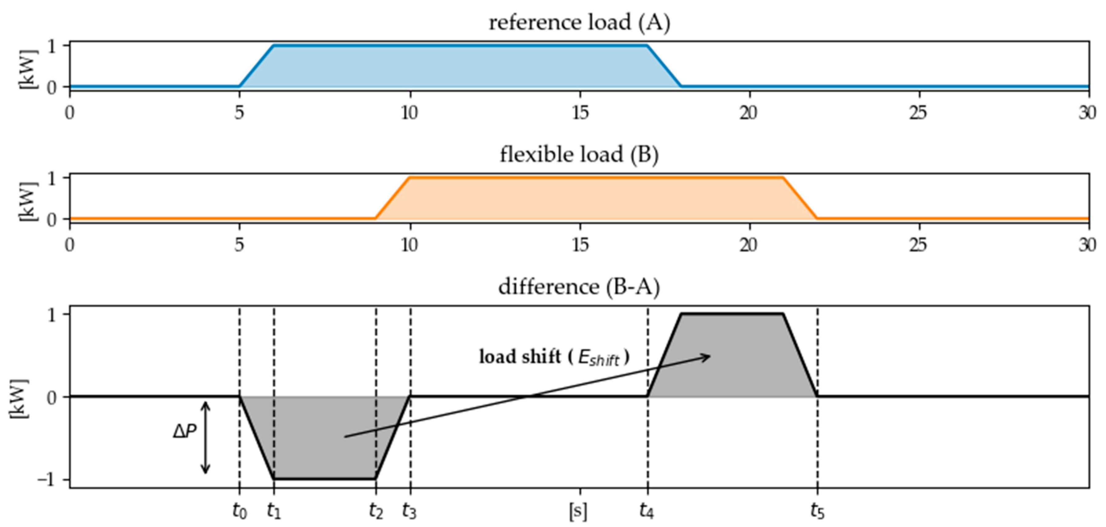
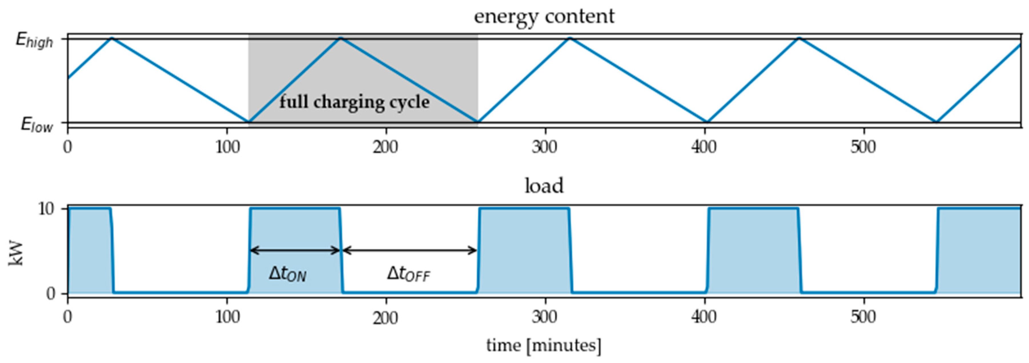
For the abovementioned example of a heated water tank in a cleaning machine, the load profile in Figure 3 is calculated. When starting the calculation, the water tank has an energy level coresponding to the initial temperature of 62.5 °C and the heating element is switched on. It should be noted, that the linearization of the curves in Figure 3 is idealized – in the case of the temperature and thus energy curve of a thermostatically controlled loads, for example, the course actually corresponds to an exponential function [37,38].

Although in order to ensure the comparability and generalizability of the substitute model, a linearization is sufficiently accurate in most cases. As outlined in the figure, each charging cycle can be characterized by the cycle time $\Delta t_{\mathrm{cycle}}$ and the load factor $a$, which is the proportion of time the energy converter is switched on during the cycle:

$$\Delta t_{\mathrm{cycle}}=\Delta t_{\mathrm{on}}+\Delta t_{\mathrm{off}}$$

(11)

$$a=\Delta t_{\mathrm{on}}/\Delta t_{\mathrm{cycle}}$$

(12)

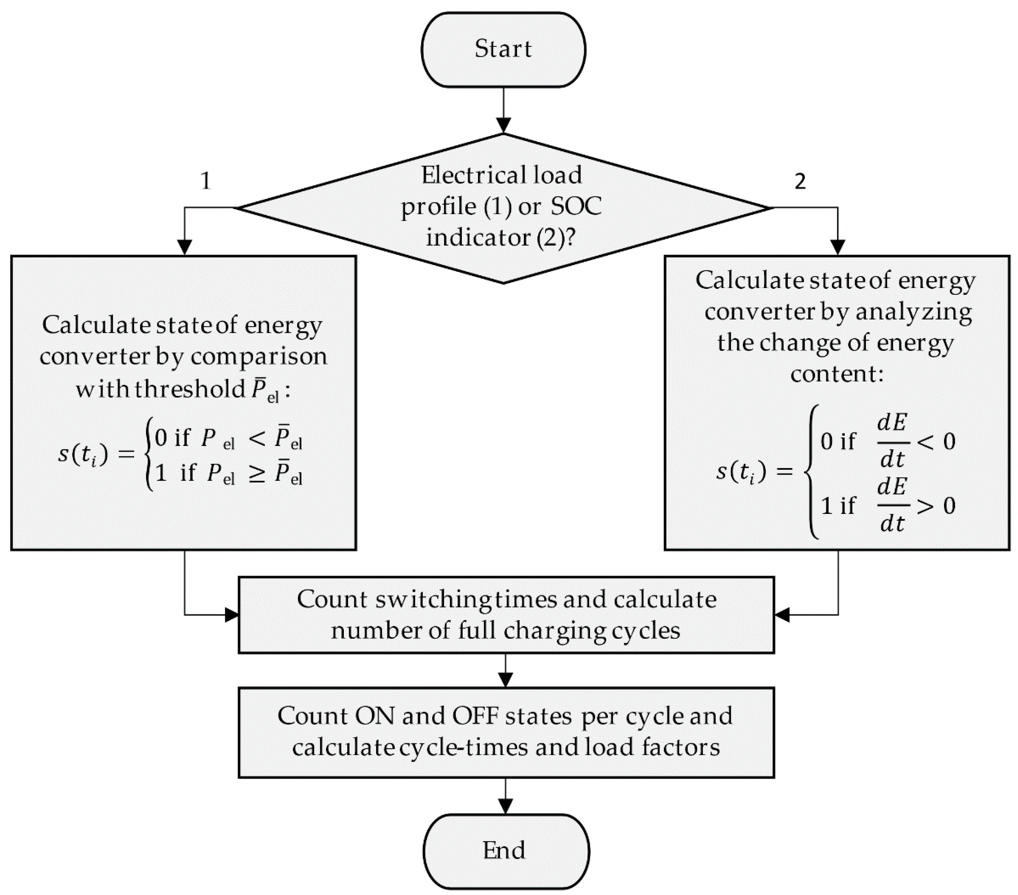
These characteristic values can be extracted from measurement data of the electric load profile of a hysteresis-controlled energy converter or its SOC indicator by the logic described in Figure 4. The logic was implemented in a load analysis function, which receives as input the measured electrical load data of the energy converter or measured data of any SOC indicator. Output of the function are the number of full charging cycles included in the considered time series, the cycle times of all recorded charging cycles as well as the respective load factor. For the example of the described heated water tank, the application of the load analysis function to the reference load profile results in a cycle duration of 144 min and a load factor of $40\%.$ These two values are later needed later to quantify the flexibility potential of the plant. The possibilities for energy-flexible operation in the case of hysteresis-controlled devices and the effects on the electrical load profile will be discussed in the next section.

2.4. Calling a Flexibility Measure

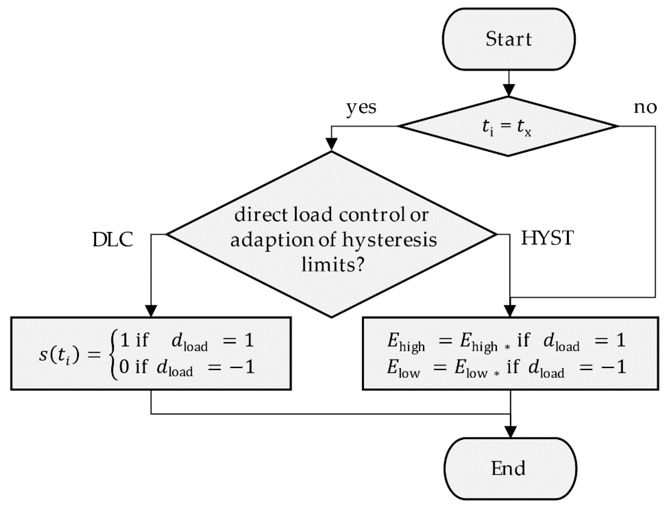
As mentioned before, there are two main options to shift the electrical load of a hysteresis-controlled device: direct load control (DLC)—thus direct switching of the energy converter—and adapting the hysteresis limits (HYST). By defining the desired call time of the flexibility measure $t_{\mathrm{x}}$ and the direction of the desired load change $d_{\mathrm{load}}$ (1 = load increase, −1 = load reduction) these two options can be implemented to calculate the flexible load profile by logic expressed in Figure 5. In case of an adaption of the hysteresis limits, the maximum upper limit of the energy content $E_{\max }$ and the minimum lower limit $E_{\min }$ must be defined in advance.

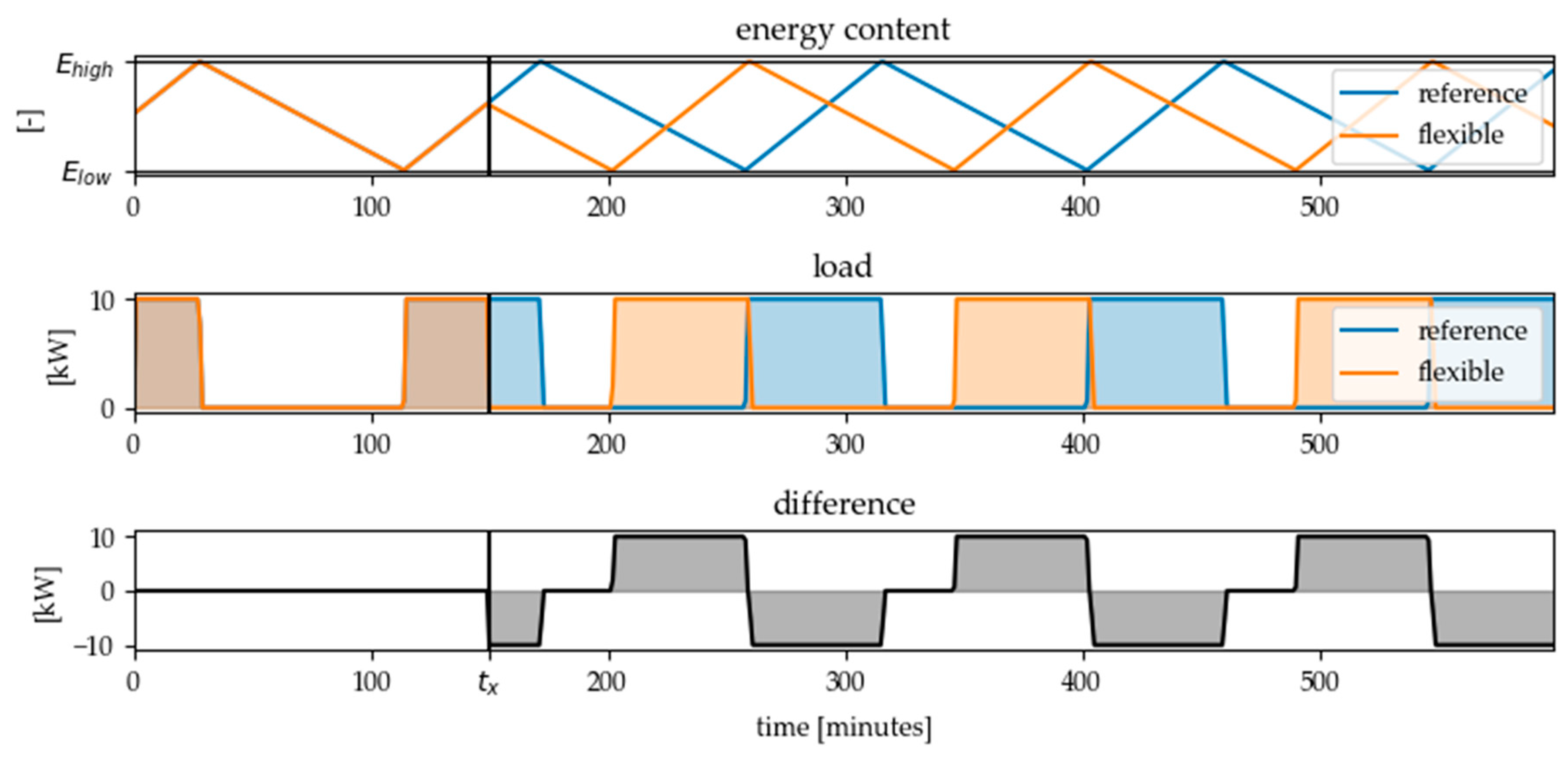
If a flexibility measure of type DLC at time step $t_x=150$ and with $d_{\mathrm{load}}=-1$ is called, a new flexible load profile can be calculated and compared to the reference load profile in normal operation mode like it is shown for the mentioned heated water tank example in Figure 6.

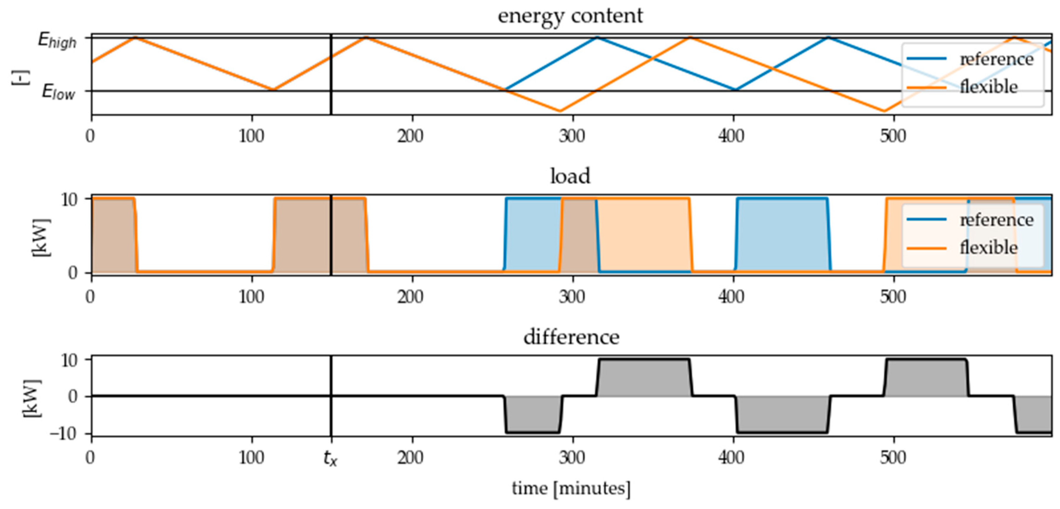
As can be seen, direct load control of the energy converter leads to an immediate reaction when the converter has the opposite state to the desired direction of load change (i.e., ON when load reduction is desired and OFF when load increase is desired). If the converter is already in the desired state, there is no reaction to the flexibility call signal. If a flexibility measure with adaption of the hysteresis limits is called at the same time and direction of load change, the flexible load profile in Figure 7 is the result. It turns out that shifting the hysteresis limits causes the desired reaction, regardless of the state of the converter at the time of flexibility call. However, the activation can be delayed, depending on when the respective limit for the energy content in the storage is reached.

Therefore in [23] it is postulated, that direct load control is suitable for short-term flexibilisation, while adaption of hysteresis limits within the initial limits can be used for long-term load shifting. It should be noted, however, that for both options the state of the energy converter at the time of retrieval plays a role. The effect of the measure on the electrical energy demand can only be calculated if the state and the electric power consumption of the energy converter is monitored and a forecast of the discharging power of the inherent storage capacity is available. In both cases (direct load control and adapting the hysteresis limits) it can be observed, that a single flexibility call causes further load changes in later time steps in addition to the desired initial load change. If these effects are not considered, they can lead to unwanted side effects such as load synchronization and avalanche effects, especially if a large fleet of similar devices is controlled by a central instance [39,40].

2.5. Method for Quantifying the State-Dependent Flexibility Potential of IES

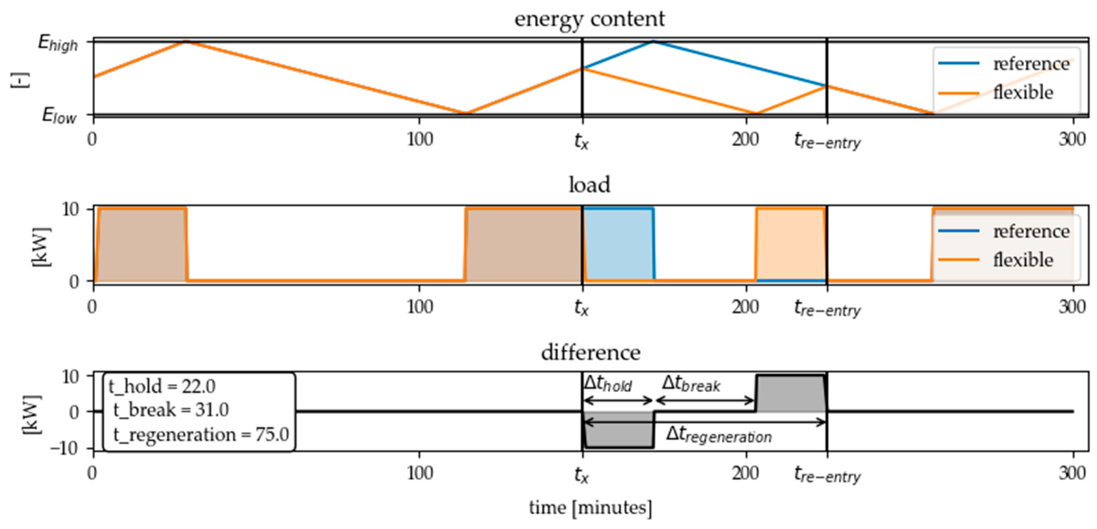
In order to counteract these unwanted further load shifts, it is possible to calculate the time at which the energy converter can re-enter the load profile in the reference case [41]. For this, the point of intersection of the reference load profile and the flexible load profile must be identified. This point ($t_{\mathrm{re}-\mathrm{entry}})$ is marked in Figure 8 for the heated water tank example. To implement this strategy in the calculation of the flexible load profile, a “reversed” call for a DLC flexibility measure which opposite load change direction compared to the original flexibility call can be inserted at $t_{\mathrm{re}-\mathrm{entry}}$. By applying this method, a defined load change can be achieved. This can be described with the standard key indicators for flexibility products. For example, the holding time of the achieved load shift is 22 min for the difference load profile shown in Figure 8. The break time between the end of the initial load reduction and the start of the corresponding load increase is 31 min and the regeneration time is 75 min. The activation and deactivation time are neglected in this example because they are less than the duration of a time step. The shifted energy amount $E_{\mathrm{shift}}$ is calculated by multiplying the holding time of the flexibility measure by the nominal electrical power of the energy converter (see Formula (13)). In the example shown, this value is $10 \mathrm{kW} ·22 \min =3.7 \mathrm{kWh}$.

$$E_{\mathrm{shift}}\left(t_x\right)=P_{\mathrm{nom},\mathrm{el}} \cdot \Delta t_{\mathrm{hold}}\left(t_{\mathrm{x}}\right)$$

(13)

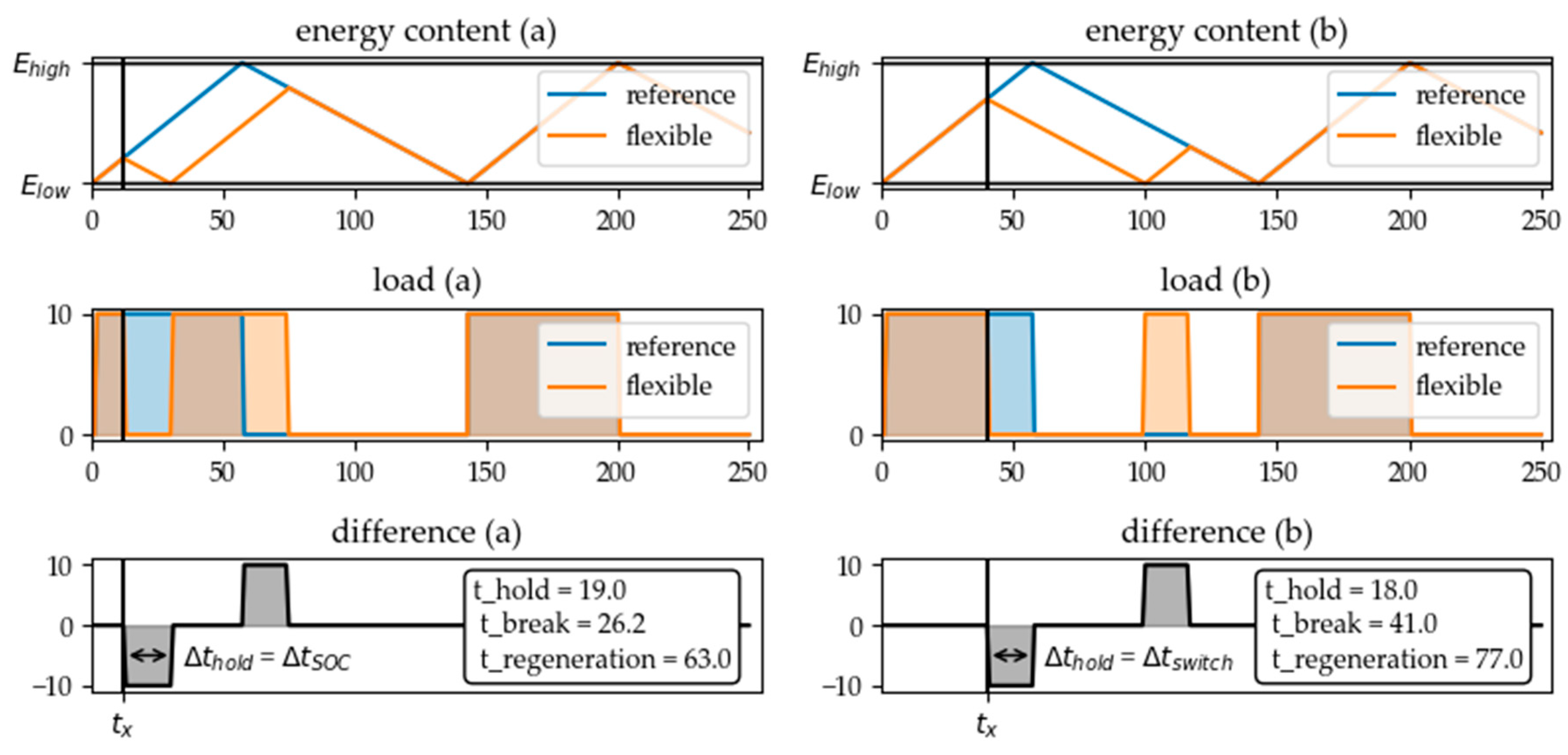
By varying the call time $t_{\mathrm{x}}$ for the flexibility measure within a charging cycle, the state-dependence of the flexibility potential of a typical hysteresis-controlled system can be analyzed in more detail. In Figure 9 can be seen that there are basically two parameters that can limit the holding time of the flexibility measure: The first one is the time interval $\Delta t_{\mathrm{SOC}}$ in which the upper or lower limit of energy content of the storage is reached in flexible operation mode (see Figure 9a). The second parameter is the time period between the flexibility call and the time step in which the energy converter would have switched the next time in normal operating mode $\Delta t_{\mathrm{switch}}$ (see Figure 9b).

These two quantities can be calculated depending on the state of the energy converter and the converter running times of the regarded charging cycle by the following system of equations:

$$\Delta t_{switch}=\{\begin{array}{c}\Delta t_{\mathrm{on}}-t_x, \mathrm{if} \mathrm{energy} \mathrm{converter} \mathrm{is} \mathrm{ON} \left(s=1\right)\\ \Delta t_{\mathrm{off}}-t_x, \mathrm{if} \mathrm{energy} \mathrm{converter} \mathrm{is} \mathrm{OFF} \left(s=0\right)\end{array}$$

(14)

$$\Delta t_{SOC}=\{\begin{array}{c}\frac{\Delta t_{\mathrm{off}}}{\Delta t_{\mathrm{on}}} ·t_x, \mathrm{if} \mathrm{energy} \mathrm{converter} \mathrm{is} \mathrm{ON} \left(s=1\right)\\ \frac{\Delta t_{\mathrm{on}}}{\Delta t_{\mathrm{off}}} ·t_x, \mathrm{if} \mathrm{energy} \mathrm{converter} \mathrm{is} \mathrm{OFF} \left(s=0\right)\end{array}$$

(15)

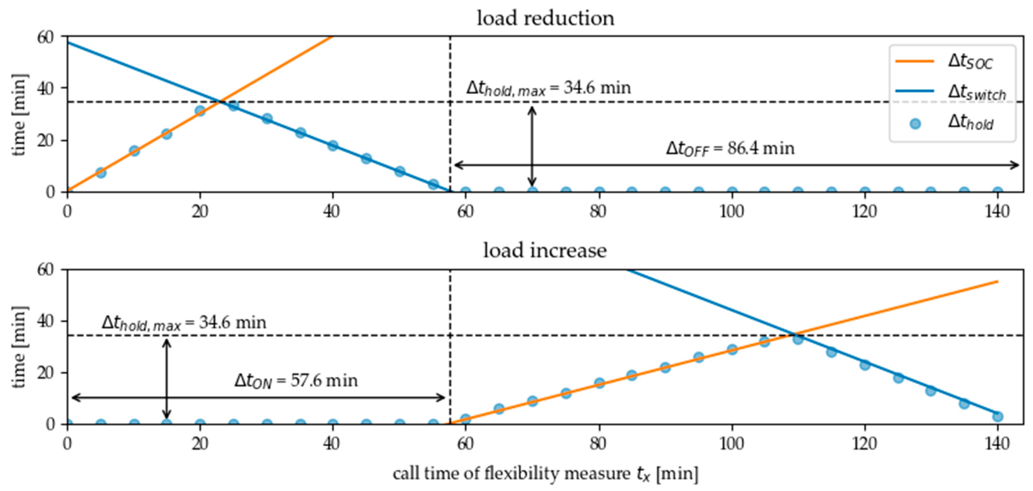
The call time of the flexibility measure $t_x$ is calculated here from the last switching time of the energy converter in normal operation. Figure 10 shows that the holding time reaches a maximum value at the time when $\Delta t_{\mathrm{switch}}$ and $\Delta t_{\mathrm{SOC}}$ are equal in case of desired load reduction as well as in case of a desired load increase. At these points in time, the amount of energy that can be shifted is maximum.

Based on this knowledge, a formula for the calculation of the maximum shiftable amount of energy, $E_{\mathrm{shift},\max }$ in dependence on the characteristical key indicators $a$ and $\Delta t_{\mathrm{cycle}}$, which can be extracted from measurement date by load analysis, is established. For calculating this energy amount, the maximum holding time must be multiplied by the nominal electrical power of the energy converter:

$$E_{\mathrm{shift},\max }=P_{\mathrm{el},\mathrm{nom}}\cdot \Delta t_{\mathrm{hold},\max }=P_{\mathrm{el},\mathrm{n}om}\cdot a\cdot \left(1-a\right) \cdot \Delta t_{\mathrm{cycle}}$$

(16)

It is also possible to calculate the times at which the flexibility measures must be activated in order to shift this maximum amount of energy:

$$t_{x, E\_\mathrm{shift},\max }=\{\begin{array}{c} a\cdot a \cdot \Delta t_{\mathrm{cycle}} \mathrm{if} \mathrm{load} \mathrm{reduction} \mathrm{is} \mathrm{required}\\ \left(1-a\right)\cdot \left(1-a\right) \cdot \Delta t_{\mathrm{cycle}} \mathrm{if} \mathrm{load} \mathrm{increase} \mathrm{is} \mathrm{required}\end{array}$$

(17)

For the example discussed with a cycle time of 144 min and a load factor of 0.4 this results in a maximum shiftable energy quantity of 5.76 kWh. Load reduction must be activated 23.04 min after switching on the energy converter, load increase after 51.84 min after switching off in order to shift this amount of energy. The cycle time and load factor are depending on the amount of useful energy required by the production process and the energy losses per time. It should be noted, however, that the amount of energy $E_{\mathrm{shift},\max }$ that can be flexibilised corresponds to the actual equivalent electrical energy content of the storage $E_{\max }$, as the following calculation shows:

$$E_{\mathrm{shift},\max }=P_{\mathrm{el},\mathrm{nom}}\cdot a\cdot \left(1-a\right) \cdot \Delta t_{\mathrm{cycle}}= P_{\mathrm{discharge},\mathrm{mean}} \cdot \Delta t_{\mathrm{OFF}}=E_{\max }$$

(18)

These equations are valid if the hysteresis limits are fixed and the flexibility is obtained by DLC. If the hysteresis limits are shifted, the flexibility potential changes as the usable energy content in the storage is changed. In addition to shifting one of the two hysteresis limits, as already mentioned above, it is also possible in some systems to shift both hysteresis limits, thus bridging the time of several charging cycles of the reference operation. This mode of operation was suggested in [42], for example, to enable hysteresis-controlled systems for load management.

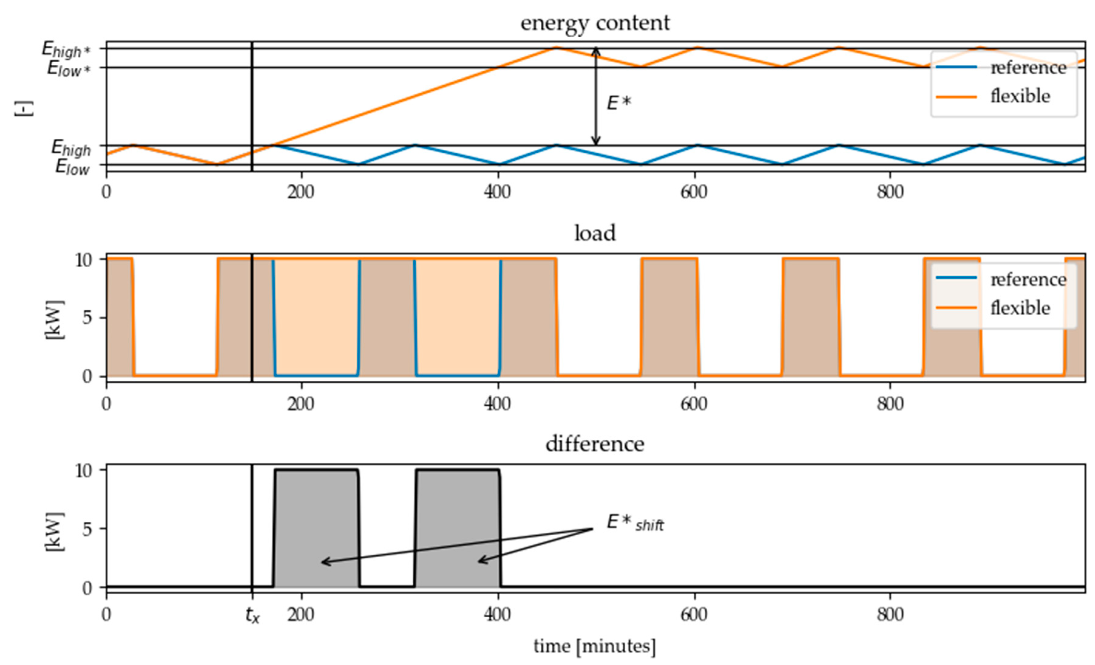
When shifting both hysteresis limits, the difference between the reference load profile and the flexible load profile, i.e., the effectiveness of the flexibility measure, can no longer be described by the standard key indicators for flexibility products. This is due to the difference between the load profile in normal operation and that in energy-flexible operation: As we see in Figure 11 at the time, where the converter would have been switched off in normal operation it stays on. Hence the difference is not constant but separated in two parts. When shifting both hysteresis limits the shiftable amount of energy consists of a state-dependent part $E_{\mathrm{shift}}\left(t_x\right)$ which describes the flexibility within the hysteresis limits and an additional, state-independent part which represents the additional energy amount $E^{*}$ due to the shift of the hysteresis limits. In addition, the amount of energy which the energy converter would have required or not required in reference mode $E_{\mathrm{el},\mathrm{ref}}$ in the period under consideration must be subtracted:

$${E^{\prime }}_{\mathrm{shift}}\left(t_x\right)=E_{\mathrm{shift}}\left(t_x\right)+E^{*}-E_{\mathrm{el},\mathrm{ref}}$$

(19)

For the example shown in Figure 11, $E_{\mathrm{shift}}\left(t_x\right)$ is zero since the energy converter is already switched on at the time step in which the load increase is called.

$E_{\mathrm{el},\mathrm{ref}}$ can be calculated from the number of full charging cycles $x$ which can be bridged by the shift of the hysteresis limits:

$$E_{\mathrm{el},\mathrm{ref}}\left(x\right)=\{\begin{array}{cc}\hfill x\cdot a\cdot \Delta t_{\mathrm{cycle}}\cdot P_{\mathrm{el}} , & \mathrm{for} \mathrm{load} \mathrm{increase} / \mathrm{increasing} \mathrm{hysteresis} \mathrm{limits}\hfill \\ \hfill x\cdot \left(1-a\right)\cdot \Delta t_{\mathrm{cycle}}\cdot P_{\mathrm{el}} , & \mathrm{for} \mathrm{load} \mathrm{reduction} / \mathrm{lower} \mathrm{hyeteresis} \mathrm{limits}\hfill \end{array}$$

(20)

The number $x$ is calculated from the ratio of the amount of energy gained by shifting the hysteresis limits to the original energy content of the storage:

$$x=\frac{E^{*}}{E_{\max }}=\frac{E^{*}{}_{\mathrm{high}}-E_{\mathrm{high}}}{E_{\mathrm{high}}-E_{\mathrm{low}}}$$

(21)

Up to a certain point, even if the hysteresis limits are shifted, the effect of the flexibility measure can still be described with the standard key figures for flexibility products. This is the case when the additional amount of energy $E^{*}$ is small, so that no complete cycle is bridged and there is no gap in the difference load profile. The following condition then applies:

$$a \cdot x \le 1 \mathrm{for} \mathrm{load} \mathrm{increase}$$

(22)

$$\left(1-a\right) \cdot x \le 1 \mathrm{for} \mathrm{load} \mathrm{reduction}$$

(23)

The described methods for quantifying the flexibility potential of hysteresis-controlled systems are validated in terms of their practical applicability in real production environments. The case study carried out for this purpose is described in the next section.

3. Case Study

The test environment for the case study is the ETA research factory at the Technical University of Darmstadt [43]. Here, a typical production chain for the metal processing industry is set up for research in energy efficiency and energy flexibility of production systems.

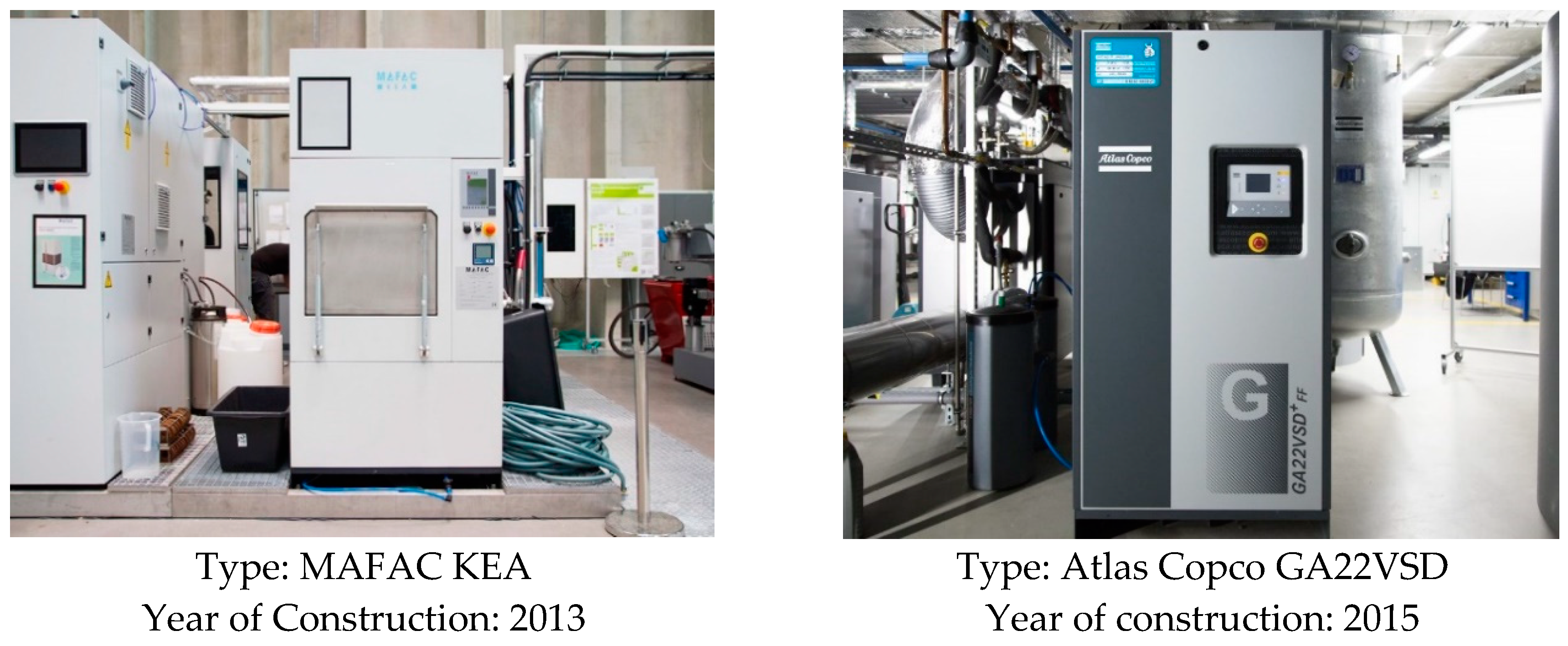
For the purpose of data acquisition, production days are regularly carried out representing real factory operations. For this study two machines are examined in detail: an industrial cleaning machine that removes oil residues and metal chips from the manufactured components and the central air compressor that supplies various production machines in the factory. In Figure 12 the two machines are shown.

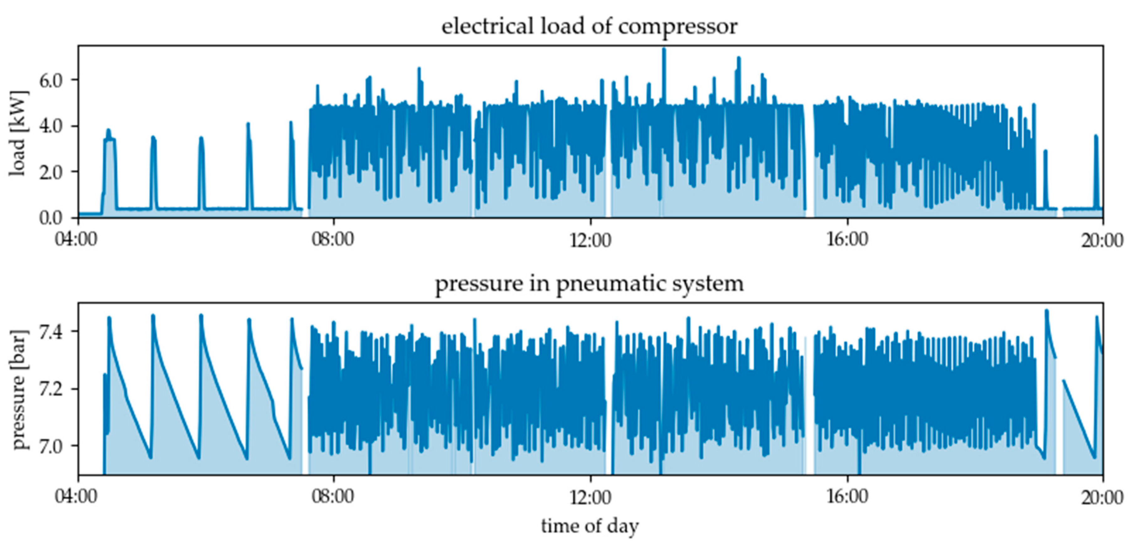
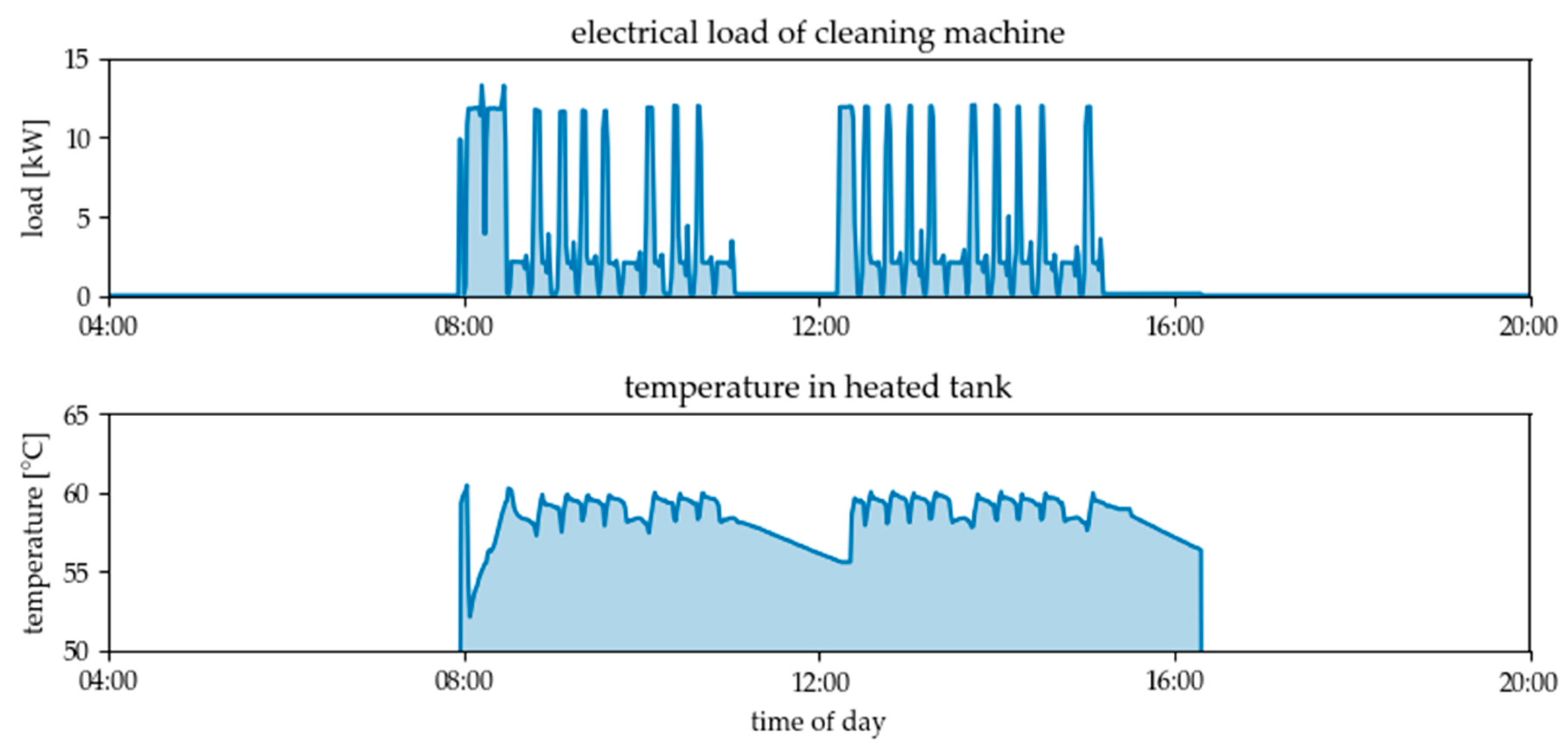
In order to quantify the flexibility potential of these two machines, the electrical load profiles were measured during one day of production operation. Since a comprehensive energy monitoring system is available in the ETA factory, which also logs data from the machine controls, the SOC indicators are also recorded. In case of the cleaning machine the SOC is calculated with the temperature in the electrical heated water tank inside the machine, in case of the air compressor it is the pressure in the compressed air network. The measured data is shown in Figure 13 and Figure 14.

The compressor starts to maintain pressure in the network before the shift starts at 08:00. When the machines are not running, it covers the losses in the pipes and the points of delivery caused by leaks. Since the flexibility potential obviously depends on whether the machines are running or not, the load analysis is carried out for two different time intervals in order to determine the characteristic values. The first interval is the time of the day during which production took place (08:00–16:00), the second is the idle time when the compressor was running and the machines were turned off (04:00–8:00). For each of these two phases and for both machines, the following steps were performed:

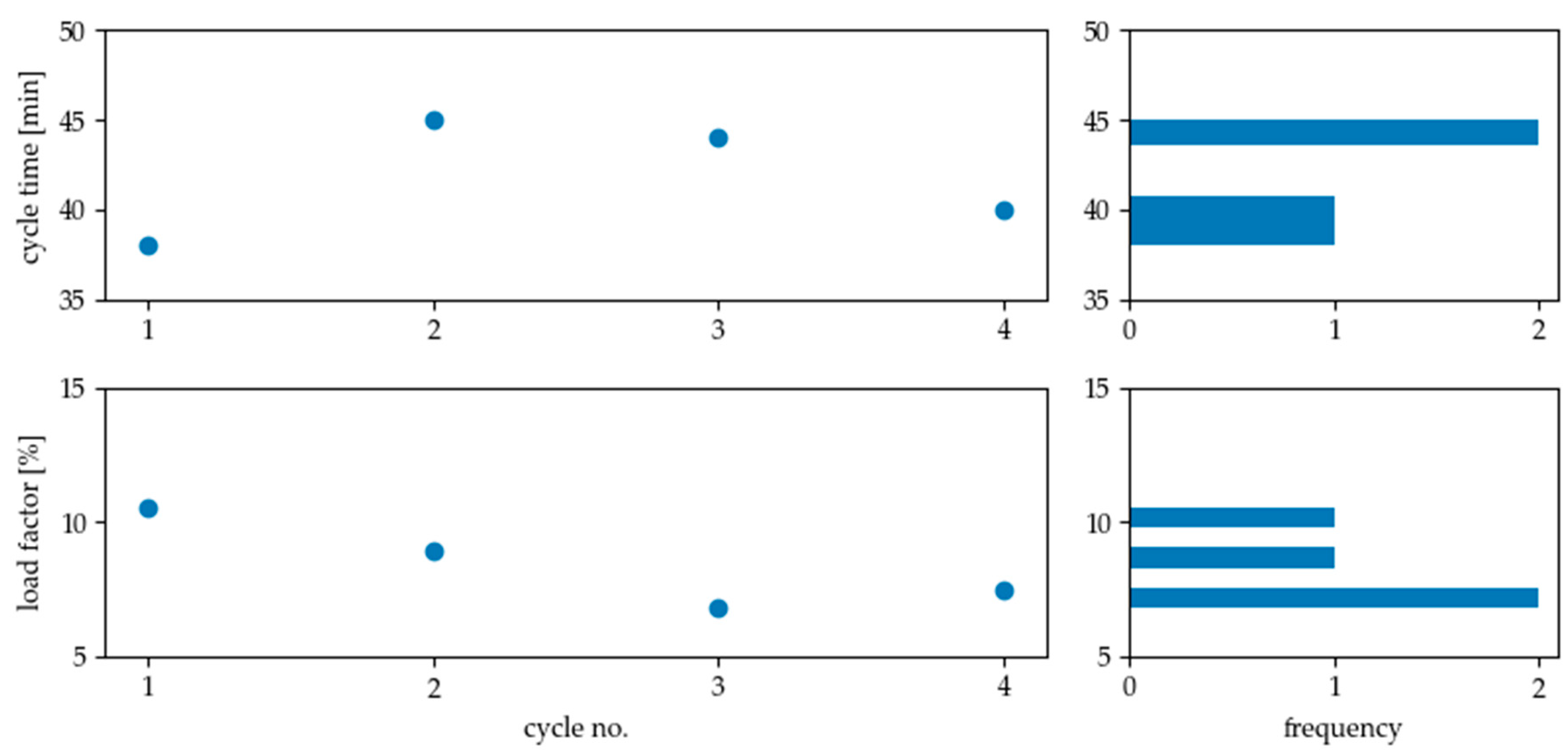
In the first step, the idling phase of the compressor between 4:00 a.m. and 7:30 a.m. is considered. Figure 15 shows that the compressor has completed a total of 4 charging cycles before the start of the shift.

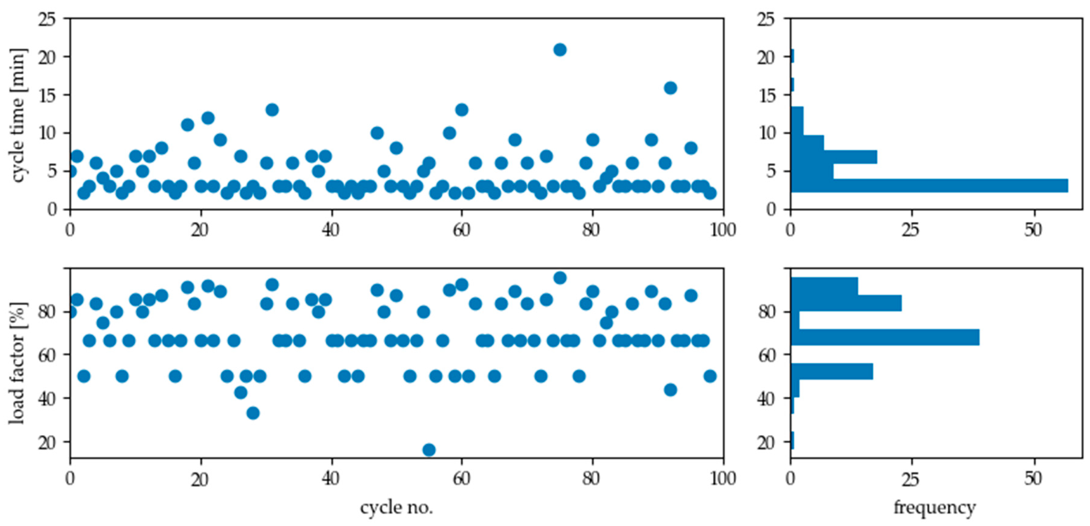
The average duration of these cycles takes 41.75 min and the mean load factor is 8.4%. This means that the compressor needs in average 3.5 min to raise the pressure in the system from the lower to the upper limit. In this case, the resulting maximum holding period for the flexibility measure is 3.2 min according to Formula (16). If a load increase is desired, the flexibility measure must be called 35.0 min after switching off the compressor in normal operation mode, load reduction has to be called 0.30 min after switching on. In order to calculate the maximum shiftable amount of energy, in addition to the holding time the electrical load of the compressor must be extracted from the measured load profile or from other information like data sheets. Here, the peak load measured is 4.13 kW between 4:00 a.m. and 7:30 a.m. With this value as nominal power, the maximum shiftable energy amount per cycle is 0.22 kWh (see Formula (16)). The procedure is similar for the other two analyzed cases. The results of the load analysis of the compressor during production (8:00 a.m. to 4:00 p.m.) are shown in Figure 16 and for the cleaning machine in Figure 17, respectively.

The results of steps 1–5 described in

Table 2. Work steps carried out in the case study.

1	Calculation of the amount of electrical energy consumed by the system (integral of the electrical load profile)
2	Measurement of the electrical load peak and average electrical power
3	Counting the full charging cycles in the considered time interval
4	Determination of the duration and load factor of the respective cycle (according to Formulas (11) and (12))
5	Calculation of the maximum shiftable amount of energy per cycle as well as the call times in case of fixed hysteresis limits (according to Formulas (16) and (17))
6	Extracting the hysteresis limits in standard operation mode from the measured data
7	Calculation of the possible flexibility potential by shifting the hysteresis limits (according to Formulas (19) and (23))

are summarized in

Table 3. Summary of the results of the case study (Step 1–5).

Key Indicators	Compressor 04:00–07:30	Compressor 08:00–16:00	Cleaning Machine 08:00–16:00
Electrical energy demand	2.47 kWh	29.40 kWh	26.31 kWh
Peak load	4.13 kW	7.34 kW	13.32 kW
Mean load	0.70 kW	3.80 kW	3.37 kW
Number of full charging cycles	4	99	19
Mean cycle time ($\Delta t_{\mathrm{cycle}}$)	41.75 min	4.8 min	21.63 min
Mean load factor ($a$)	8.4%	69.7%	25.8%
Maximum holding time of flexibility measure ($\Delta t_{\mathrm{hold},\max }$)	3.22 min	1.02 min	4.12 min
Call time for load increase ( $t_{x, E\_\mathrm{shift},\max }$)	35.01 min	0.44 min	11.91 min
Call time for load reduction ( $t_{x, E\_\mathrm{shift},\max }$)	0.30 min	2.35 min	1.44 min
Shiftable energy amount per cycle ($E_{\mathrm{shift}, \max }$)	0.22 kWh	0.12 kWh	0.92 kWh
Total shiftable energy amount	0.88 kWh	11.88 kWh	17.48 kWh
Share of flexible energy in energy demand	35.6%	40.1%	66.3%

. The largest flexibility potential can be identified for the cleaning machine during production. The air compressor has a lower shiftable energy amount per cycle, but theoretically this can be activated more often due to the greater number of cycles.

A detailed discussion of the results was conducted in Section 4. It must be emphasized that the air compressor is a device with the possibility of partial load operation. The extent to which this should be taken into account when calculating the potential for flexibility should be analyzed in future work. Furthermore, in the case of the cleaning machine, it was not the flexible auxiliary unit (the tank heating) that was measured, but the total electrical power consumed by the machine. Although the switch-on times of the tank heating can be clearly identified from the load profile, it would still be necessary to analyze how large the base load share of the electrical power requirement of the machine is, which could distort the result.

In addition to the flexibility potential within the existing hysteresis limits of the systems, there is also the possibility of gaining flexibility by shifting the hysteresis limits (step 6–7). For the two machines in the ETA research factory, the following shifts are available after consultation with the plant managers:

▪

Compressor: Increase of the upper pressure level up to 8 bar possible

▪

Cleaning machine: Extension of the upper hysteresis limit up to 68 °C is possible

Under the assumption that the additional energy amount gained by shifting the hysteresis limits can be extrapolated linearly, the values summarized in

Table 4. Summary of the results of the case study (Step 6–7).

Key Indicators	Compressor 04:00–07:30	Compressor 08:00–16:00	Cleaning Machine 08:00–16:00
Upper limit of SOC Indicator	7.46 bar	7.45 bar	60.47 °C
Lower limit of SOC Indicator	6.95 bar	6.88 bar	57.29 °C
Hysteresis range in normal operation	0.51 bar	0.57 bar	3.18 °C
Limit value for the increase factor of energy content 1 $\left(x\right)$	$\frac{1}{0.084}=11.90$	$\frac{1}{0.697}=1.43$	$\frac{1}{0.258}=3.88$
New possible hysteresis range 1	6.07 bar	0.82 bar	12.34 °C
New possible upper limit of SOC Indicator 1	13.53 bar	8.27 bar	72.81 °C
New upper limit of SOC Indicator 2	8.00 bar	8.00 bar	68 °C
Actual increase factor of the energy content $\left(x\right)$ 3	$\frac{8.00 \mathrm{bar}-7.46 \mathrm{bar} }{0.51 \mathrm{bar}}=1.06$	$\frac{8.00 \mathrm{bar}-7.45 \mathrm{bar} }{0.57 \mathrm{bar}}=0.96$	$\frac{68 °\mathrm{C}-60.47 °\mathrm{C}}{3.18 °\mathrm{C}}=2.37$
Additional amount of energy $\left(E^{*}\right)$	$1.06\cdot 0.22 \mathrm{kWh}=0.23 \mathrm{kWh}$	$0.96\cdot 0.12 \mathrm{kWh}=0.12 \mathrm{kWh}$	$2.37\cdot 0.92 \mathrm{kWh}=2.18 \mathrm{kWh}$

¹ Limit value up to which it is possible to describe the flexibility potential of load increase using standard key figures, see Equation (22). ² The maximum values given by experts are below the theoretically possible values, which is why they were used for the further calculation. ³ Assuming a constant efficiency of the converter over time and linear dependence between SOC indicator and storage content.

can be calculated for the new flexibility potentials in this case.

4. Discussion and Conclusions

The presented methodology for quantifying the flexibility potential of inherent energy storages respectively hysteresis-controlled devices in production systems offers a framework that is transferable to different types of machines or other devices. With the developed substitute model, the devices can be benchmarked against each other in terms of their flexibility potential and the flexible energy amount can be calculated in the form of the standard key figures of flexibility products on the energy markets. With the presented method it is possible to calculate the flexibility potential automated from the electrical load profiles of the energy converters or measurements of the respective SOC indicator. This will enable integration into energy monitoring systems in the future.

The case study which has been carried out for an industrial cleaning machine and an air compressor shows a flexibility potential of 0.92 kWh and 0.12 kWh, respectively, which can be shifted per charging cycle during production time. The maximum holding times of the flexibility measures are 4.12 respectively 1.02 min. As the cycle time of the compressor is significantly shorter than that of the tank heating of the cleaning machine, its flexibility potential can be called up more frequently per day. Over the entire production period of 8 h, this results in a flexible energy quantity of 11.88 kWh for the compressor and 17.48 kWh for the cleaning machine. If a shift of the upper hysteresis limits for both systems were implemented within the limits specified by the plant managers, the additionally gained, state independent flexibility potential is $0.12 \mathrm{kWh}$ per charging cycle for the compressor during production time and $2.18 \mathrm{kWh}$ per cycle for the heated tank of the cleaning machine. For both installations, the effectiveness of the flexibility measure can still be described using the standard indicators for energy flexibility measures described in Section 2.2 in this case.

To evaluate these results, typical energy contents of classical electrical energy storage systems can be used as a reference. For example, the size of a battery for scheduling the electrical power consumption of households with photovoltaics ranges between as 5.5 kWh [44] and 13.5 kWh [45]. The energy content of a mobile phone battery like the Apple iPhone 11 is about 0.012 kWh [46] and a the battery capacity of a laptop like the Lenovo Thinkpad T490s is 0.057 kWh [47].

It thus becomes clear that the flexibilisable energy quantities of inherent energy storage in production systems are certainly within a relevant range, especially when considering the number of these systems installed. However, the amounts of energy can only be shifted at certain points in time and, at least for the examples considered, only for relatively short time periods. Whether it is economical for companies to make these flexibilities available to the electricity market depends on the effort it takes to enable the machines. As a guideline, in which cases an investment could be worthwhile, a comparison with classic electrical energy storage systems can also be used here. According to [48] the investment sum for a lead acid battery with a capacity of 11.88 kWh amounts to 13,500 €—so such a battery with the same capacity as the flexible energy amount of the cleaning machine per cycle (0.92 kWh + 2.18 kWh = 3.1 kWh) would cost roughly 3500 €. For lithium ion batteries, the authors quote an amount of 52,500 € for a system with a capacity of 40 kWh—with this specific cost, the investment for a storage capacity of 3.1 kWh would be 4100 €. This rough calculation does not take into account the fact that ageing effects and wear are likely to play a greater role in electrical energy storage systems than in an electrically heated water tank designed for cyclic operation. However, the prices for lithium ion batteries are currently falling steadily. According to [49] they are around 100 €/kWh, [50] forecasts a value of 84 €/kWh for the year 2020. With these values the investment for a storage capacity of 3.1 kWh would only be 260–310 €.

Besides financial aspects, an evaluation of the ecological sense is also possible in this way. According to [48], the resource expenditure for the construction of 14 lead acid batteries results in a greenhouse gas emission of 8718.13 kg CO₂ equivalent. Converted to a capacity of 3.1 kWh, this would result in 162.5 kg CO2 equivalent if a new electrical battery would be produced instead of using the flexibility potential of the cleaning machine, which already exist. This idea will be further developed in subsequent research work. In addition, it will be analyzed how a flexible operation affects the efficiency of the devices—for example, heat losses increase when the bath temperature of cleaning machines is increased, which was not considered in the present study. The developed tool for load analysis will be improved in further work, especially regarding the partial load behavior of the devices and the use of advanced data analysis techniques. For example, clustering methods can be used to identify time spans with regular cycle times and thus reliably available flexibility potentials. The developed procedure for the extraction of the characteristic values of IES from measurement data is to be tested in the ETA research factory in real operation, in which the algorithm continuously updates the flexibility potential of the devices. This will provide further insights into how the approaches can be applied under real network conditions. In particular, an analysis of the reliability of the forecasts of the useful energy demand and thus of the possible call times for the maximum flexibility potential will be examined more closely.

Finally, the aggregation of the potential of several flexible devices in larger production facilities as well as the optimal composition of these plant pools in terms of different goals of demand side management will be investigated in future work. This is particularly interesting with regard to a possible use of the flexibility potential of IES in the field of ancillary services. A large number of IES, whose flexibility is aggregared, can provide flexibility in both load directions through the stochastic distribution of their system states. In addition, in large plant pools forecast uncertainties of the individual plant my be compensated by other devices. This can increase reliability and thus the suitability for the provision of control power.

References

- Connolly, D.; Lund, H.; Mathiesen, B.V. Smart Energy Europe: The technical and economic impact of one potential 100% renewable energy scenario for the European Union. Renew. Sustain. Energy Rev. 2016, 60, 1634–1653. [Google Scholar] [CrossRef]
- Samad, T.; Koch, E.; Stluka, P. Automated Demand Response for Smart Buildings and Microgrids: The State of the Practice and Research Challenges. Proc. IEEE 2016, 104, 726–744. [Google Scholar] [CrossRef]
- Ulbig, A.; Andersson, G. Analyzing operational flexibility of electric power systems. Int. J. Electr. Power Energy Syst. 2015, 72, 155–164. [Google Scholar] [CrossRef]
- Alizadeh, M.I.; Parsa Moghaddam, M.; Amjady, N.; Siano, P.; Sheikh-El-Eslami, M.K. Flexibility in future power systems with high renewable penetration: A review. Renew. Sustain. Energy Rev. 2016, 57, 1186–1193. [Google Scholar] [CrossRef]
- BDEW. Stromverbrauch in Deutschland Nach Verbrauchergruppen 2019. Available online: https://www.bdew.de/media/documents/Nettostromverbrauch_nach_Verbrauchergruppen_2019_online_o_jaehrlich_Ki_12032020.pdf (accessed on 22 April 2020).
- Torriti, J.; Hassan, M.G.; Leach, M. Demand response experience in Europe: Policies, programmes and implementation. Energy 2010, 35, 1575–1583. [Google Scholar] [CrossRef] [Green Version]
- Li, B.; Shen, J.; Wang, X.; Jiang, C. From controllable loads to generalized demand-side resources: A review on developments of demand-side resources. Renew. Sustain. Energy Rev. 2016, 53, 936–944. [Google Scholar] [CrossRef]
- Council of the EU Directive (EU). 2019/944 on Common Rules for the Internal Market for Electricity and Amending Directive 2012/27/EU: 2019. Available online: https://eur-lex.europa.eu/eli/dir/2019/944/oj (accessed on 10 August 2020).
- Wattjes, F.D.; Janssen, S.L.L.; Slootweg, J.G. Framework for estimating flexibility of commercial and industrial customers in Smart Grids. In Proceedings of the IEEE PES ISGT Europe 2013, Lyngby, Denmark, 6–9 October 2013; IEEE: Piscataway, NJ, USA, 2013; pp. 1–5. [Google Scholar]
- Petersen, M.K.; Edlund, K.; Hansen, L.H.; Bendtsen, J.; Stoustrup, J. A taxonomy for modeling flexibility and a computationally efficient algorithm for dispatch in Smart Grids. In Proceedings of the 2013 American Control Conference, Washington, DC, USA, 17–19 June 2013; IEEE: Piscataway, NJ, USA, 2013; pp. 1150–1156. [Google Scholar]
- Deng, R.; Yang, Z.; Chow, M.-Y.; Chen, J. A Survey on Demand Response in Smart Grids: Mathematical Models and Approaches. IEEE Trans. Ind. Inf. 2015, 11, 570–582. [Google Scholar] [CrossRef]
- VDI. Energieflexible Fabrik: Grundlagen (VDI 5207 Blatt 1); Beuth Verlag: Berlin, Germany, 2019. [Google Scholar]
- Schoepf, M.; Weibelzahl, M.; Nowka, L. The Impact of Substituting Production Technologies on the Economic Demand Response Potential in Industrial Processes. Energies 2018, 11, 2217. [Google Scholar] [CrossRef] [Green Version]
- Zhang, X.; Hug, G.; Kolter, Z.; Harjunkoski, I. Industrial demand response by steel plants with spinning reserve provision. In Proceedings of the 2015 North American Power Symposium (NAPS), Charlotte, NC, USA, 4–6 October 2015; IEEE: Piscataway, NJ, USA, 2015; pp. 1–6. [Google Scholar]
- Zhang, X.; Hug, G.; Harjunkoski, I. Cost-Effective Scheduling of Steel Plants with Flexible EAFs. IEEE Trans. Smart Grid 2017, 8, 239–249. [Google Scholar] [CrossRef]
- Otashu, J.I.; Baldea, M. Scheduling chemical processes for frequency regulation. Appl. Energy 2020, 260, 114125. [Google Scholar] [CrossRef]
- Bohlayer, M.; Fleschutz, M.; Braun, M.; Zöttl, G. Energy-intense production-inventory planning with participation in sequential energy markets. Appl. Energy 2020, 258, 113954. [Google Scholar] [CrossRef]
- Summerbell, D.L.; Khripko, D.; Barlow, C.; Hesselbach, J. Cost and carbon reductions from industrial demand-side management: Study of potential savings at a cement plant. Appl. Energy 2017, 197, 100–113. [Google Scholar] [CrossRef]
- Rohde, C. Erstellung von Anwendungsbilanzen für die Jahre 2018 bis 2020 für die Sektoren Industrie und GHD; Fraunhofer Society: Karlsruhe, Germany, 2019. [Google Scholar]
- Shoreh, M.H.; Siano, P.; Shafie-khah, M.; Loia, V.; Catalão, J.P.S. A survey of industrial applications of Demand Response. Electr. Power Syst. Res. 2016, 141, 31–49. [Google Scholar] [CrossRef]
- Eisenhauer, S.; Reichart, M.; Sauer, A.; Weckmann, S.; Zimmernann, F. Energieflexibilität in der Industrie: Eine Metastudie; Institut für Energieeffizienz in der Produktion, Universität Stuttgart: Stuttgart, Germany, 2018. [Google Scholar]
- Conte, F.; Massucco, S.; Silvestro, F.; Ciapessoni, E.; Cirio, D. Stochastic modelling of aggregated thermal loads for impact analysis of demand side frequency regulation in the case of Sardinia in 2020. Int. J. Electr. Power Energy Syst. 2017, 93, 291–307. [Google Scholar] [CrossRef]
- Wai, C.H.; Beaudin, M.; Zareipour, H.; Schellenberg, A.; Lu, N. Cooling Devices in Demand Response: A Comparison of Control Methods. IEEE Trans. Smart Grid 2015, 6, 249–260. [Google Scholar] [CrossRef]
- Koch, S.; Zima, M.; Andersson, G. Active Coordination of Thermal Household Appliances for Load Management Purposes. IFAC Proc. Vol. 2009, 42, 149–154. [Google Scholar] [CrossRef] [Green Version]
- Rui, X.; Liu, X.; Meng, J. Dynamic Frequency Regulation Method Based on Thermostatically Controlled Appliances in the Power System. Energy Procedia 2016, 88, 382–388. [Google Scholar] [CrossRef] [Green Version]
- van der Heijde, B.; Sourbron, M.; Arance, F.V.; Salenbien, R.; Helsen, L. Unlocking flexibility by exploiting the thermal capacity of concrete core activation. Energy Procedia 2017, 135, 92–104. [Google Scholar] [CrossRef] [Green Version]
- Stadler, I. Demand Response: Nichtelektrische Speicher für Elektrizitätsversorgungssysteme mit Hohem Anteil Erneuerbarer Energien; Habilitation, der Universität Kassel: Berlin, Germany, October 2006. [Google Scholar]
- Koch, S.; Mathieu, J.; Callaway, D.S. Modeling and control of aggregated heterogeneous thermostatically controlled loads for ancillary services. Proc. PSCC 2011, 1–7. Available online: http://citeseerx.ist.psu.edu/viewdoc/summary?doi=10.1.1.460.6240 (accessed on 10 August 2020).
- Sterner, M.; Stadler, I. Energiespeicher-Bedarf, Technologien, Integration; Springer: Berlin/Heidelberg, Germany, 2017. [Google Scholar]
- Bundesamt für Energie BFE. Kälte Effizient Erzeugen: Das Wichtigste Zur kälteerzeugung Nach SIE 382/1; Bern, Switzerland, 2016; Available online: https://pubdb.bfe.admin.ch/de/publication/download/8559 (accessed on 10 August 2020).
- Gloor, R. Druckluftsysteme: Kennzahlen und Informationen über Energiesparmöglichkeiten bei Druckluftanlagen. Available online: https://energie.ch/druckluft/ (accessed on 24 April 2020).
- DIN Deutsches Institut für Normung e.V. Energetische Bewertung von Gebäuden—Lüftung von Gebäuden: Teil 3: Lüftung von Nichtwohngebäuden (DIN EN 16798-3:2017); Beuth Verlag GmbH: Berlin, Germany, 2017. [Google Scholar]
- Kuhrke, B. Methode Zur Energie-und Medienbedarfsbewertung Spanender Werkzeugmaschinen. Zugl.: Darmstadt. Ph.D. Dissertation, Technival University of Darmstadt, Berlin, Germany, 2011. [Google Scholar]
- Heemels, W.; Lehmann, D.; Lunze, J.; Schutter, B. Introduction to hybrid systems. In Handbook of Hybrid Systems Control: Theory, Tools, Applications; Cambridge University Press: Cambridge, UK, 2009; pp. 3–30. [Google Scholar]
- European Network of Transmission System Operators for Electricity (ENTSO-E). Electricity Balancing in Europe: An Overview of the European Balancing Market and Electricity Balancing Guideline; ENTSO-E: Brussels, Belgium, 2018. [Google Scholar]
- Oldewurtel, F.; Borsche, T.; Bucher, M.; Fortenbacher, P.; Gonzalez Vaya, M.; Haring, T.; Mathieu, J.L.; Mégel, O.; Vrettos, E.; Andersson, G. A framework for and assessment of demand response and energy storage in power systems. In Proceedings of the 2013 IREP Symposium Bulk Power System Dynamics and Control-IX Optimization, Security and Control of the Emerging Power Grid, Rethymnon, Crete, Greece, 25–30 August 2013; IEEE: Piscataway, NJ, USA, 2013; pp. 1–24. [Google Scholar]
- Moura, S.; Bendtsen, J.; Ruiz, V. Parameter identification of aggregated thermostatically controlled loads for smart grids using PDE techniques. Int. J. Control 2014, 87, 1373–1386. [Google Scholar] [CrossRef]
- Qu, Z.; Xu, C.; Ma, K.; Jiao, Z. Fuzzy Neural Network Control of Thermostatically Controlled Loads for Demand-Side Frequency Regulation. Energies 2019, 12, 2463. [Google Scholar] [CrossRef] [Green Version]
- Angeli, D.; Kountouriotis, P.-A. A Stochastic Approach to “Dynamic-Demand” Refrigerator Control. IEEE Trans. Contr. Syst. Technol. 2012, 20, 581–592. [Google Scholar] [CrossRef]
- Postnikov, A.; Albayati, I.M.; Pearson, S.; Bingham, C.; Bickerton, R.; Zolotas, A. Facilitating static firm frequency response with aggregated networks of commercial food refrigeration systems. Appl. Energy 2019, 251, 113357. [Google Scholar] [CrossRef]
- Popp, R.S.-H.; Liebl, C.; Zaeh, M.F. Energy Flexible Machine tool Components—An Investigation of Capabilities. Procedia CIRP 2016, 57, 692–697. [Google Scholar] [CrossRef]
- Xie, K.; Hui, H.; Ding, Y. Review of modeling and control strategy of thermostatically controlled loads for virtual energy storage system. Prot. Control Mod. Power Syst. 2019, 4, 23. [Google Scholar] [CrossRef]
- Abele, E.; Beck, M.; Flum, D.; Schraml, P.; Panten, N.; Junge, F.; Bauerdick, C.; Helfert, M.; Sielaff, T. Gemeinsamer Schlussbericht zum Projekt ETA-Fabrik Energieeffiziente Fabrik für Interdisziplinäre Technologie-und Anwendungsforschung; Technische Universität Darmstadt: Darmstadt, Germany, 2019. [Google Scholar]
- Sonnen. Technische Daten sonnenBatterie 10. Available online: https://media.sonnen.de/de/media/62/download/inline (accessed on 14 May 2020).
- Tesla. Powerwall: Die Powerwall-Ihr Stromspeicher. Available online: https://www.tesla.com/de_DE/powerwall (accessed on 14 May 2020).
- GSMArena. Apple iPhone 11. Available online: https://www.gsmarena.com/apple_iphone_11-9848.php (accessed on 15 May 2020).
- Osthoff, A. Test Lenovo ThinkPad T490s (i5, Low-Power-FHD) Laptop. Available online: https://www.notebookcheck.com/Test-Lenovo-ThinkPad-T490s-i5-Low-Power-FHD-Laptop.416248.0.html (accessed on 15 May 2019).
- VDI Zentrum Ressourceneffizienz. Ökologische und Ökonomische Bewertung des Ressourcenaufwands: Stationäre Energiespeichersysteme in der Industriellen Produktion, 2nd ed.; VDI Zentrum Ressourceneffizienz: Berlin, Germany, 2018. [Google Scholar]
- Arcos-Vargas, Á.; Canca, D.; Núñez, F. Impact of battery technological progress on electricity arbitrage: An application to the Iberian market. Appl. Energy 2020, 260, 114273. [Google Scholar] [CrossRef]
- Nier, H. Preisverfall bei Lithium-Ionen-Batterien. Available online: https://de.statista.com/infografik/20280/preisentwicklung-von-lithium-ionen-batterien/ (accessed on 4 August 2020).
Figure 1.
Simplified substitute model of an inherent energy storage consisting of the energy converter, which converts electricity into the energy form required by the production process and the inherent storage capacity.
Figure 2.
The effectiveness of a flexibility measure from the electricity grids’ point of view is calculated according to [12] from the difference between the load profile in normal operation (reference load) and the one in energy flexible operation (flexible load).
Figure 3.
Resulting reference load profile for a heated water tank (volume = 1 m3, temperature hysteresis = 5 K, nominal electrical power of heating element = 10 kW, discharging power = 40% of nominal electrical power constantly).
Figure 4.
Program flow chart of the load analysis function for extraction of the characteristic values from measured data of the electrical power of the energy converter or the SOC indicator.
Figure 5.
Program flow chart of calling a flexibility measure to calculate the flexible load profile.
Figure 6.
Resulting flexible load profile for a flexibility call of type DLC (Direct Load Control) at time step = 150 and a desired load reduction ( ) in comparison to the reference load profile without flexibility call.
Figure 7.
Resulting flexible load profile for a flexibility call of type HYST (adapting hysteresis limits) at time step = 150 and a desired load reduction () in comparison to the reference load profile without flexibility call.
Figure 8.
By defining the re-entry-point in the reference load profile (intersection of the reference load and the flexible load profile), a defined load shift can be achieved. This can be quantified by the standard key indicators for flexibility products.
Figure 9.
Two parameters can limit the holding time of the flexibility measure: The time interval in which the limit of energy content of the storage is reached in flexible operation mode (a) or the time until the next switching time in reference mode is reached (b).
Figure 10.
Holding time of the flexibility measure in dependence of the call time of the flexibility measure within one charging cycle. In normal operation the energy converter is switched on from time step 0 to 57.6, thus the measure of load reduction is available in this period. Load increase can only be called in the second part of the charging cycle time.
Figure 11.
Load difference when shifting both hysteresis limits at the same time. The figure shows the results for the heated water tank example when shifting the temperature limits from 60–65 °C to 85–90 °C.
Figure 12.
Cleaning machine (left) and compressed air genereator (right) in the ETA-Factory.
Figure 13.
Electrical load profile of the compressed air generator and pressure in the network on 13.02.2019.
Figure 14.
Electrical load profile of the cleaning machine and temperature in the heated water tank on 13.02.2019.
Figure 15.
Result of load analysis for compressor in standby operation (4 a.m. to 7.30 a.m.). Each dot in the left pictures represents a full charging cycle. On the right side, the frequency with which the respective values occurred is shown. The resulting average cycle time is 41.75 min, the mean load factor 8.4%.
Figure 16.
Result of load analysis for compressor during production (8 a.m to 4 p.m). The resulting average cycle time is 4.83 min, the mean load factor of all full cycles is 69.7%.
Figure 17.
Result of load analysis for cleaning machine during production (8 a.m to 4 p.m). The resulting average cycle time is 21.63 min, the mean load factor of all full cycles is 25.8%.