Development of an Integrated Simulation Model for Load and Mobility Profiles of Private Households

Abstract

The electrification of the mobility and heating sectors will significantly change the electrical behavior of households in the future. To investigate this behavior, it is important to include the heating and mobility sectors in load profile models. Existing models do not sufficiently consider these sectors. Therefore, this work aims to develop an integrated, consistent model for the electrical and thermal load of private households and their mobility behavior. The model needs to generate regionally distinct profiles depending on the building, household and resident type and should be valid for Germany. Based on a bottom-up approach, a model consisting of four components is developed. In an activity model based on a modified Markov chain process, persons are assigned to activities. The activities are then allocated to devices in the electrical and thermal models. A mobility model assigns distances to the journey activities. The results of the simulation to validate the model shows an average annual energy consumption per household of 2751 kWh and a shape of the average load profile, both in good agreement with the reference. Furthermore, the temporal distribution of the vehicles to the locations is in accordance with the reference but the annual mileage is slightly underestimated with 10,730 km.

1. Introduction

The energy transition is placing new demands on distribution grids in Germany. On the one hand, many renewable energy systems, e.g., photovoltaic systems, have been installed and on the other hand, load has also risen and is expected to rise further due to the electrification of the mobility and heating sectors [1,2]. Both developments are mainly taking place in the distribution grid and especially in low voltage grids [3]. Combined with digitalization, which enables producers and consumers to be more easily controlled, these developments are leading to new challenges and opportunities for electricity grids. Detailed simulation models are necessary to learn more about, and to develop solutions for, these upcoming challenges. One crucial factor, therefore, is a realistic and accurate model for the electrical consumption as well as mobility and heating demands of households, which are or will be the main source of electrical load in low voltage grids. To achieve this, three interwoven types of demand must be taken into account. First is the common electrical load of devices in the household, for example, ovens, televisions, and laptops. Second is the heating demand for space heating and hot water, which is increasingly frequently provided by heat pumps. The third is the mobility demand of the inhabitants, which, in the future, can be fulfilled by electric cars. Since these three demands are linked together via the user behavior, e.g., if the person of a single household is driving to work, the electric and thermal load in the empty home normally decreases, an integrated model shall be developed.

Due to the highly relevant nature of the problem, there is already a large number of models to generate electric load profiles of households. The authors of [4] give a general overview of existing models for this topic. Accordingly, those models can be classified in bottom-up and top-down approaches. A common and very simple top-down method is to use a standard load profile (SLP). These are average load curves based on long-term-measurements for weekdays and weekend days. The German Association of Energy and Water Industrie (BDEW) provides an SLP for German households in a temporal resolution of 15 min [5]. The main disadvantages of this method are its inaccuracy when considering a small number of households and its relatively low temporal resolution [6]. Slightly more precise top-down models are described in [7,8]. Reference [4] categorizes both as deterministic statistical disaggregation models, because they use measured load profiles but disaggregate the profiles to determine various appliance. The simple parametrization used in both cases is advantageous, as is the low computing effort featured in one case. On the other hand, both cases lack detail and diversity.

Bottom-up models first calculate the electric demand of single devices and then aggregate or extrapolate these values to obtain the total consumption of individual households or a larger geographic area. They can be divided into statistical random, probabilistic empirical, and time-use-based models [4]. Statistical random models use statistical data in combination with a random procedure to achieve diversity. The authors of [9] developed such a model. Besides electric load profiles, it also generates domestic hot water and space heating demand. This model was criticized by [4,10] because of its simplicity and its meaningless validation. Reference [11] describes a probabilistic empirical model that uses statistical total load curves and load curves of electric devices, as well as socioeconomic data, as input data. Based on that data, the triggering probabilities of the devices are calculated. However, the influence of the user’s presence was neglected [10]. Time-use-based models consider user presence based on data from time-use-surveys to generate diversity. Time-use surveys measure the amount of time people spend performing various activities through interviews and protocols. The authors of [12] combined this method with a deterministic approach, by using the time-use data directly. Other references like [13] use the data to calculate transition probabilities for a Markov chain beforehand, from which they compute synthetic activity profiles. Afterwards, these profiles are linked with load profiles of electric devices to determine the load profile of the household. The author of [10] decided against using Markov chains and generated the synthetic activity profiles with the help of a probability distribution instead.

The next step is to present some existing approaches of mobility models. Reference [14] describes a deterministic model based on the 2008 “mobility in Germany” (MiD) study [15]. This study consists of 30,000 daily mobility profiles which were clustered in user groups and various types of days. The model randomly picks a profile for a person of the related user group and day. There is a large variety of mobility models based on Markov chains similar to the previously-mentioned models for load profiles [16,17,18]. An approach with three parking states and one driving state is utilized in [16]. Using time-use data, the model assigns one of the states to each car in every time step. Thus the duration of the journey is determined. The distance is calculated by the average speed. A multiple driving states Markov model with 13 different states is presented in [17]. Each driving state represents a trip reason. Reference [18] uses a spatial Markov chain model that combines geographical information system (GIS) data with a Markov chain process. The model distinguishes between three parking states: Work, Home, and Other. Geospatial maps are used to estimate the distances of each journey. The authors in [19] combined a trip chain model with a Markov chain model.

Models like [16,17,18] already used the mobility models to estimate future system perturbation of electromobility. Thus, they combine mobility and electric load profiles in their models. The only model which already combines mobility, heating demand and electric load profiles is [10]. However, the used mobility model is highly simplified and the results are very questionable. It generates an annual driving distance, ranging from 2000 to 18,000 km and averaging 3000 km, for each car present in the model. In comparison, the average value provided by the German Federal Motor Transport is around 14,000 km [20].

The consideration of related work showed a wide variety of existing models, but also revealed their deficits. Upon reviewing these, the requirements of the model developed in this paper can be defined as follows:

• Consistent mobility, heating demand, and electric load profiles
• Regionally distinct results depending on the building, household, and resident type
• Mobility behavior consistent with city size
• Huge diversity of profiles
• High temporal resolution of one minute

By developing a model that meets these requirements, this paper helps to fill the research gaps that remain after considering similar models.

The aim is to create an integrated bottom-up model, which can generate mobility, heating demand, and electric load profiles. These profiles need to be consistent. For example, it is unlikely that a one-person household will generate an electric peak load while the resident is traveling by car. However, a peak load is very likely to occur when returning by switching on electrical appliances and charging the electric vehicle. Therefore, it is important to link the profiles to activities in order to achieve this consistency.

The model must reflect regional differences. Through different types of buildings, households, and residents, regional differences must be producible. Thus, various types of settlements from different regions can be simulated. In addition, there is a strong deviation of the mobility behavior in rural and urban regions. The model must display this difference as well. To examine peak loads and the corresponding grid load, the diversity of the load profiles is very important. Average load profiles would be inappropriate for this purpose. The model must provide this diversity. At least for the electric load profile, a temporal resolution of one minute is mandatory for the same reason.

The work is structured as follows: in chapter two, the methods of the individual model components activity, electric load, thermal load, and mobility are described. Using a simulation of a representative German settlement, the results of the model components are validated and discussed in the third chapter. The paper ends with a short conclusion in chapter four.

2. Methodology

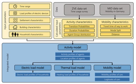
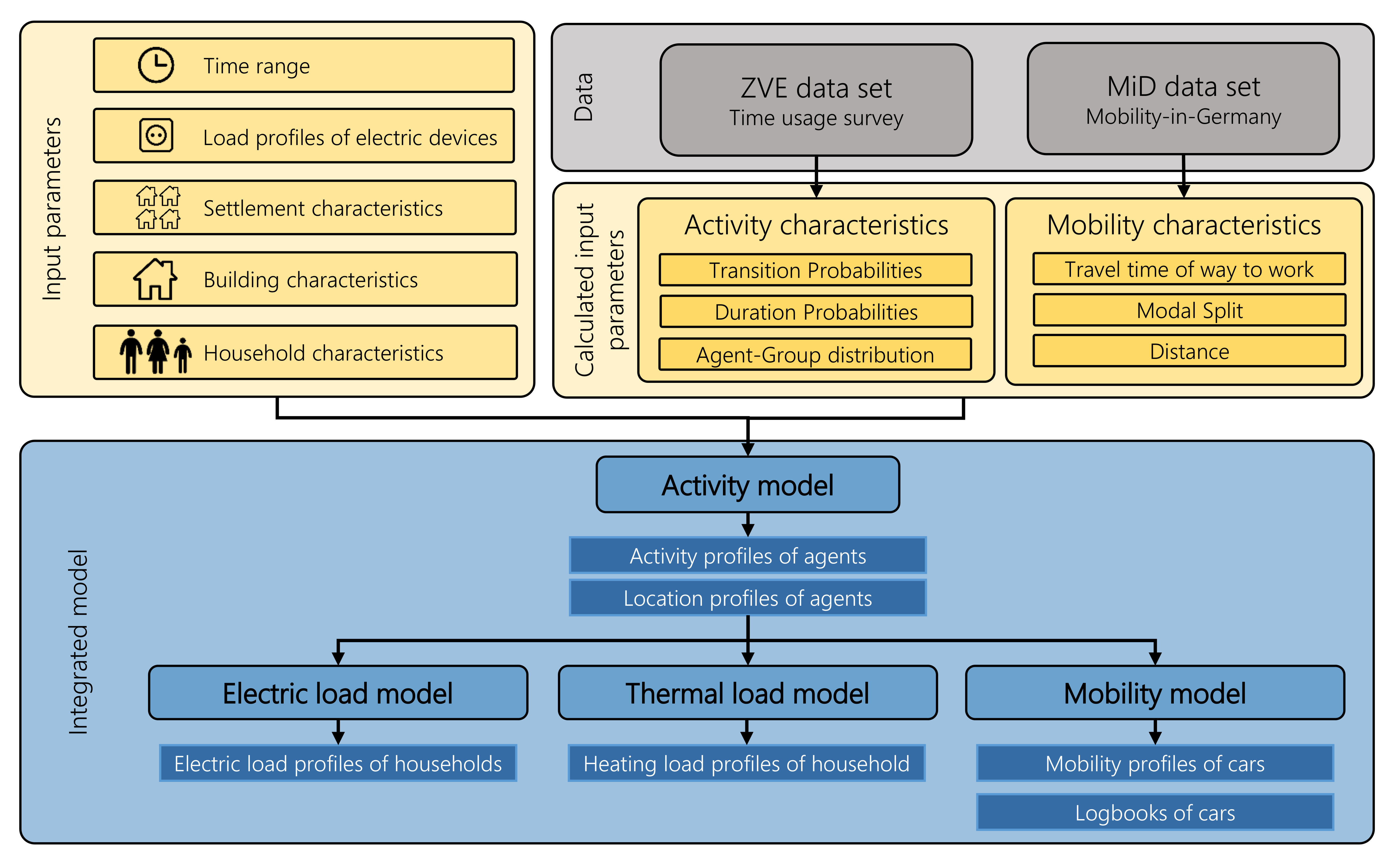
This section describes the model which is developed within this paper. It consists of four parts: the activity model, the mobility model, the electric load model, and the thermal load model. The models are also called generators in some cases. Figure 1 shows a general overview of the model. There are two types of input data. On the one hand, there are input parameters that characterize the buildings, households and persons the profiles will be generated for. On the other hand, there are probabilities and distributions that characterize the activity and mobility behavior of different types of persons. Those inputs are determined based on studies that are representative of German citizens. The data inputs for the activity behavior are based on a time-use survey (ZVE) [21] and those for the mobility behavior on the mobility study MiD. Using the input data, the activity model produces activity profiles for each resident of the regarded building. The residents are referred to as agents. An agent group is a group of agents with the same characteristics. The activity profiles are passed on to the other three parts of the model. The electric load model links the activity profiles with profiles of electric devices and trigger-probabilities to generate electric load profiles of the residential units. Residential units and households are synonymous with this work. The thermal load model similarly assigns activities to a demand for hot water. The heating demand is not coupled to the activity profiles. The mobility model generates mobility profiles for the cars of each household based on the activity profile of its residents.

At this point, the defined input parameters will be explained before the following subsections describe the single components of the model in detail. The first parameter is the time range for which the load profile will be generated. The maximum time range is one year and the minimum time range is one day. Because of the temporal resolution of the used data sets, the activity and the mobility model uses time steps of 10 min. For the load models, the activities are repeated to achieve a temporal resolution of 1 min. The model is developed to generate load- and mobility-profiles at the settlement level. Therefore a settlement, which contains buildings, which contain, in turn, residential units, needs to be defined by certain parameters.

Table A1. Input Parameters at the level of settlement, building and residential.

Level	Name	Value	Description	Distrb. in %
Settlement	City category	1	Rural region: ≤ 50.000 residents	100
		2	City: from 50.000 to 450.000 residents	0
		3	Large city: from 450.000 to 650.000 residents	0
		4	Metropolis: ≥ 650.000 residents	0
	Number of houses	≤ 1	Number of houses the settlement consists of	/
Building	Building type	1	One family house	57.77
		2	Duplex house	2.67
		3	Terraced house	6.67
		4	Two family house	3.33
		5	Apartment house (3–6 residential units)	8.33
		6	Apartment house (7–12 residential units)	19.67
		7	Apartment house (≤ 1 residential units)	2.67
	Building age	1	Built before 1900	4.67
		2	Built between 1900 and 1945	31.67
		3	Built between 1946 and 1960	14
		4	Built between 1961 and 1970	14.67
		5	Built between 1971 and 1980	8
		6	Built between 1981 and 1985	4
		7	Built between 1986 and 1995	10
		8	Built between 1996 and 2000	8.33
		9	Built between 2001 and 2005	4.33
		10	Built after 2006	0.33
Building	Number of residential units	≤ 1	Numer of residential units within a building	/
	Living space	/	Living Space of the building in $m^2/RU$	/
	Specific heating demand	/	Specific heating demand of the building in $kWh/m^2$	/
	Level of refurbishment	0	No refurbishment	33
		1	Conventional refurbishment	33
		2	Future-orientated refurbishment	34
Household	Household size	1	Number of persons within the residential unit	37.13
		2		33.19
		3		14.47
		4		10.43
		5		4.79
	Household type	1	see Table 4	29.36
		2		44.04
		3		13.19
		4		9.57
		5		1.17
		6		2.66
	Electric equipment	1	small	33
		2	middle	33
		3	full	34
	Bathtub available	yes	The residential unit has a bathtub	70
		no		30
	Consumption level	1	Low consumption level for electricity and hot water	33
		2	Medium consumption level for electricity and hot water	33
		3	High consumption level for electricity and hot water	34
	Car available	yes/no	The residential unit has a car	100

contains a description of these parameters. The settlement itself is defined by the number of buildings and the city category (CC). Through the city category, differences between the activity and mobility behavior of the rural and urban populations are considered. A settlement must contain at least one building. The buildings are characterized by parameters such as their age, type and living space. The number of residential units within a building is a parameter as well. The parameter household size and type are responsible for the assignment of agents to the residential units.

Table 1. Allocation logic of household parameters to agents.

Household size	1	1	1	1	1	1	2	2	2	2	3	3	3	4	4	4	5	5	5
Household type	1	2	3	4	5	6	1	2	3	4	1	2	3	1	2	3	1	2	3
Full time working man	1						1		1		1	1		1	1		1	1
Full time working woman		1					1			1	1		1	1		1	1		1
Male pensioner			1					1
Female pensioner				1				1
Part time working man					1					1			1			1			1
Part time working woman						1			1			1			1			1
Children											1	1	1	2	2	2	3	3	3

contains the allocation logic based on [21]. The input distinguishes between seven types of agents from which the households are built. The parameters’ electric equipment, consumption level and the availability of a bathtub are important to model the load behavior of a residential unit. The decision of whether the household owns a car is implemented by another parameter.

2.1. Activity Model

Time-use surveys are generally statistics, which include information about how people spend their time. In this case, the time-use survey ZVE of the German Federal Statistical Office from 2012/2013 is used. Over 5000 representative households with more than 11,000 individuals were interviewed during the survey. The interviews consisted of household interviews, personal interviews, and diaries, which collected the detailed daily routine of the respondents in time steps of ten minutes for three days (two weekdays and one weekend day). Within the household interview, attributes like the number of individuals living in the household and the living space were determined. Personal information like age, gender, and marital and social status was collected through personal interviews. The activities from the collected diaries were clustered into 165 defined activity categories. The social status of the respondents was clustered in categories (Freelancer, Civil Servant, Employee, Worker, Pupil/Student, Pensioner, Unemployed) as well. Additionally, the data set contains information about the labor situation (full-time, part-time) of each respondent and whether the person does shift work. [21,22]

Even though the data set was already prepared by the German Federal Statistical Office, some interventions were necessary to make the data usable for a modified Markov process. Activities lasting for a whole day—for example, if the person is sick in bed or away on a journey—had to be removed, because they could lead the activity generator to a dead end. It affected only 0.004% of the data. The journeys to and from work were removed as well to achieve a constant expenditure of time for these activities. A Markov chain could not reach that requirement. Therefore, commutes are subsequently inserted. Furthermore, the activity categories of the original data set (165) are too extensive. Hence, they were clustered into 19 activity categories, which are shown in

Table 2. Activity categories used in the model.

ID	List of Activities	Impact on	Location
01	Sleeping	Presence/absence	Home
02	Eating	Presence/absence	Home/work/other place
03	Hygiene and dressing	Electricity and water consumption	Home
04	Meal preparation	Electricity consumption	Home
05	Baking	Electricity consumption	Home
06	Dish-washing	Electricity and water consumption	Home
07	Cleaning up home	Electricity and water consumption	Home
08	Doing the laundry	Electricity and water consumption	Home
09	Ironing	Electricity consumption	Home
10	Watching TV	Electricity consumption	Home
11	Listening to the radio	Electricity consumption	Home
12	Using the computer	Electricity consumption	Home
13	Other activities at home	Presence/absence	Home
14	Working	Presence/absence	Home/work
15	Education	Presence/absence	Home/other place
16	Social contacts	Presence/absence	Home/other place
17	Other activities	Presence/absence	Other place
18	Not at home	Presence/absence	Other place
19	Other journey	Presence/absence	Other journey
20	Commute	Presence/absence	Commute

. For example, the ZVE includes different types of work. e.g., main job, secondary job, etc. These are all grouped together in the activity “Work”. Like in [10], days from Monday to Thursday are aggregated because of their similar daily routine. As a result, the model distinguishes between four types of days (ToD): Monday-Thursday, Friday, Saturday and Sunday.

Based on the upper criteria shown in

Table 3. Criteria to filter the time-use study representative for Germany (Zeitverwendungserhebung) (ZVE) data.

Criteria	Symbol	Definition Area	Distinctions
Gender	/		Male/female
Social status	/		Freelancer/civil servant/employee/ Worker/student/pensioner
Labour situation	/		Full time/part time
Shift work	/		Yes/no
Activity	i	$\{1,2,\dots ,19\}$	See Table 4
Activity after i	j	$\{1,2,\dots ,19\}$	See Table 4
Time of day	t	$\{1,2,\dots ,144\}$	144 time steps with 10 min each
Activity duration	T	$\{1,2,\dots ,144\}$	Number of time steps t the activity i lasts
Type of day	$ToD$	$\{1,2,3,4\}$	Monday-Thursday (1), Friday(2), Saturday (3), Sunday (4)

, 21 detailed agent groups are defined. The data set is divided into partial diary data sets for each agent group, which can be found in

Table 4. Itemisation of the agent-groups.

Agent-Group Input	p	Detailed Agent-Groups
Full time working man	0.13	Male full-time freelancer
	0.12	Male full-time civil servant
	0.57	Male full-time employee
	0.06	Male full-time worker with shift work
	0.12	Male full-time worker without shift work
Full time working women	0.13	Female full-time freelancer
	0.12	Female full-time civil servant
	0.57	Female full-time employee
	0.06	Female full-time worker with shift work
	0.12	Female full-time worker without shift work
Male pensioner	1	Male pensioner
Female pensioner	1	Female pensioner
Part time working man	0.13	Male part-time freelancer
	0.12	Male part-time civil servant
	0.57	Male part-time employee
	0.18	Male part-time worker without shift work
Part time working women	0.13	Female part-time freelancer
	0.12	Female part-time civil servant
	0.57	Female part-time employee
	0.12	Female part-time worker without shift work
Children	1	Student

.

The cumulative activity transition probability $p_{TR,j,t,ToD}\left(i\right)$ is calculated by Equation (1) similar to [13]. Therefore, the relative frequency is assumed as probability. Here, i is the activity during the time step t, j is the activity during the previous time step $t-1$ and $ToD$ is the type of day. $n_{j,t,ToD}$ is the number of persons who change on a day-type $ToD$ and at time step t from activity j to another activity. The counter variable k is used to determine the cumulative sum of the probabilities for each activity i. Thus, $n_{j,t,ToD}\left(k\right)$ is the number of persons who change from activity j to activity k at t on $ToD$. If there are no persons meeting the criteria, the probability is zero. The definition area for the variables j, t and $ToD$ is contained in Table 3.

$$p_{\mathrm{TR},j,t,ToD}\left(i\right)=\left\{\begin{array}{cc}\sum _{k=1}^i\frac{n_{j,t,ToD}\left(k\right)}{n_{j,t,ToD}}\hfill & ,n_{j,t,ToD}\ne 0\hfill \\ 0\hfill & ,n_{j,t,ToD}=0\hfill \end{array}\right.$$

(1)

A typical Markov approach recalculates the activity based on probabilities for every time step without having information about the activity of the previous time step. An example of the activity sleeping can be used to illustrate the disadvantages of a Markov process. Assuming a constant probability for sleeping of 0.98, the probability that an agent sleeps for six hours (36 time steps) would be only ${0.98}^{36}=0.48$. Thus, in a regular Markov process, the probability that agents get up for a short time and then continue sleeping is very high. To avoid this, the duration probability $p_{TR,j,t,ToD}\left(i\right)$ of activities are additionally calculated by Equation (2). T is the duration of activity i and the counter variable k runs from 1 to T. Thus, for each agent group 4-dimensional probability matrices for transition and duration are calculated. These form the basis for the following modified Markov process.

$$p_{\mathrm{DU},i,t,ToD}\left(T\right)=\left\{\begin{array}{cc}\sum _{k=1}^T\frac{n_{i,t,ToD}\left(k\right)}{n_{i,t,ToD}}\hfill & ,n_{j,t,ToD}\ne 0\hfill \\ 0\hfill & ,n_{i,t,ToD}=0\hfill \end{array}\right.$$

(2)

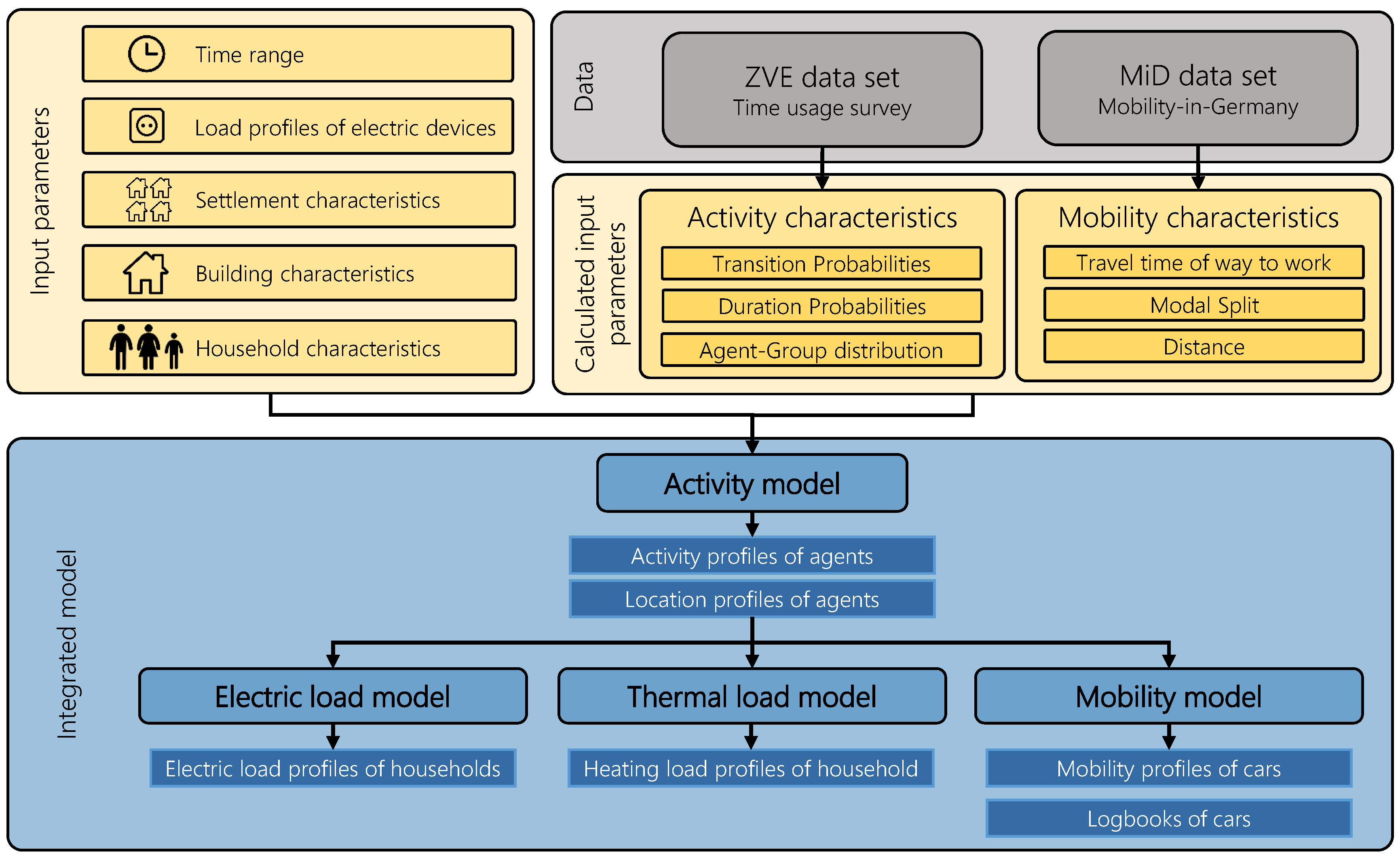
Figure 2 shows the procedure within the activity model. The model iterates over every agent and time step. The first step is the refinement of the agent groups. Children and Pensioners can be allocated explicitly. The remaining agent groups are refined based on the probabilities included in Table 4. Thus, the inserted agent groups are allocated to the detailed agent groups of the ZVE.

For the first activity and its duration, real values from the ZVE-data set from a respondent of the corresponding agent group are used. After the first activity ends, the actual algorithm starts by generating a single uniformly distributed random number r within the interval 0 and 1. The probabilities for a transition from the present activity to another activity for the present time step and $ToD$ are extracted out of the transition probability matrix $p_{TR}$. The result is a vector with 19 entries. Each entry represents an activity. The algorithm iterates over the activity-entries to find the first entry which is greater than or equal to r. This is the new activity i. Afterward, the duration of the new activity is determined similarly. Another random number r is generated. The probabilities for the duration of the present activity, time step, and $ToD$ are selected from the duration probability matrix $p_{DU}$. The algorithm assigns the duration of the new activity based on the probability matrix. After the activity has ended, the algorithm is repeated until the last time step is reached. The activity vector is the result of the first part of the model. In every time step, the agent is linked to one of the activities from Table 2. Afterward, the missing commutes are added to achieve a constant duration for that activity. The first and the last time step of all working-time-blocks are determined. Within a working-time-block, which is the range of time in which the agent works, there can be interruptions like eating or other activities. The algorithm recognizes these blocks. The commute from home to work starts at the first entry of the working-time-block. The commute back home is included backward starting from the last entry of the block. The duration-distribution of the commute is based on the mobility data introduced in Section 2.4. The used distribution depends only on the city category.

The next step is to link the activities to locations. The location of each agent at each time step is stored in a location vector. The model distinguishes between five locations: “at home”, “at work”, “other location”, “other journey”, and “commuting”. Commuting includes the way from and to work. Most of the activities can be explicitly coupled to one location. Table 2 contains the assumed, possible locations for each activity. For example sleeping (ID = 01) is explicitly linked to the location at home. Other activities like eating (ID = 02) can not be unambiguously assigned to a location. Agents can eat at home, at work or at other locations. The model assigns these indefinite locations by checking the locations before and after them. For example, if the agent is at work before and after the activity eating, he will remain there to eat.

Table A2. Assignment of locations to activities with indefinite location.

Before	After	Present
Home	Home	Home
Home	Work	Home
Home	Other location	Home
Home	Other journey	Home
Home	Commute	Home
Work	Home	Work
Work	Work	Work
Work	Other location	Work
Work	Other journey	Work
Work	Commute	Work
Other location	Home	Work
Other location	Work	Work
Other location	Other location	Work
Other location	Other journey	Work
Other location	Commute	Work
Other journey	Home	Home
Other journey	Work	Work
Other journey	Other location	Other location
Other journey	Other journey	Other location
Other journey	Commute	Other journey
Commute	Home	Home
Commute	Work	Work
Commute	Other location	Other location
Commute	Other journey	Other journey
Commute	Commute	Work

contains the used assignments.

It is assumed that the agent does not return home within a working-time-block. Thus, every location-entry in the mobility vector which is home between the way to work and the way back home is corrected to the location at work.

For the mobility model, a meaningful location profile is very important. To achieve that, the following requirements are defined:

• Transitions between at home, at work, and another location require a journey (commute or another journey) among it.
• Direct transitions from home to another location to home are allowed.
• The duration of the other journey from home to another location has to be equal to the following trip back home.

The first requirement is necessary to avoid that the car, which may be used for a later trip within the mobility model, is led to a dead end. The second requirement is defined, because there are activities linked to other locations that do not require a journey. For example, another activity contains sports. It is not necessary to change the location to go jogging. The activity can start and end at home, even though it happens at other locations. To generate realistic distances in the mobility model, the third requirement is mandatory. Section 2.4 will further explain the necessity of requirements 1 and 3. The algorithm scans the location vector and checks whether the requirements are fulfilled. If not, the vector is processed to meet them. Missing journeys with a duration of one-time step are included in case of a violation of requirements 1 and 2. If necessary, the travel times are reduced or extended to meet the third requirement.

The last step of the activity model is the harmonization of the activity and the location vector. Every entry in the activity vector with a location at work or at another place is set to not at home (id = 18). Activity entries with a location, other journey, or commute are changed to the activity with the same name. The outputs of the activity model are an activity vector and a location vector.

2.2. Thermal Load Model

In addition to electricity, thermal energy is needed in all households. Therefore, thermal energy is also part of the described model. The thermal load model consists mainly of modules regarding the use of thermal energy at home. The first module is heating and the second one is hot water.

The module for heating demand is rather simple and is described in detail in [23]. Therefore the specific heating demand of the building, which depends on age, level of refurbishment, and type is the starting point. Based on this value, according to [24,25], using the standard load profile procedure for gas customers, the annual space heating requirement is distributed over the individual days of the year, taking into account the weighted temperature of the last three days and the type of building. This gives a space-heating requirement for each day of the year. The standard load profile for gas is used since heating dominates the gas consumption and gas is an energy source which is delivered just in time to many customers. Unfortunately, there is not much data available for district heating, which would be another good source for heating demand profiles. The model also takes into account that new buildings only need to be heated from an average daytime temperature below 14 °C and older buildings from less than 15 °C. In the last step, the daily heating requirements are distributed over the day using distribution functions according to [26]. This results in a heat demand profile in an hourly resolution for the chosen building.

The second module, for hot water, is quite similar to the electric load model in Section 2.3 and takes the different activities into account. Instead of the probabilities of using electrical devices, however, tapping probabilities of the individual hot water tapping points derived from the previously generated activity profiles are used here. The consumption values per tapping event, i.e., required volume flow rate and tapping duration, are taken from [27]. The required heat demand is derived from the required volume flow rate and the tapping temperature, which is dependent on the respective draw-off point. In order to maintain realism, restrictions based on the frequencies of use in [28], the shower and the bathtub are used per person, maximally once a day. In addition, calibration factors are used to adjust the consumption. The modeling of the usage is similar to the electrical one. There are possibilities for all activities (see Table 2), which are related to hot water consumption, like cleaning up home or dish-washing, that hot water is needed. In this case, the selected possibilities are compared to a random number. Retrieval of the withdrawal point only takes place if the random number exceeds a certain value. The possibilities were calibrated according to the demands in [29].

2.3. Electric Load Model

The Electric Load Model is based on the described Activity Generator and aims to generate an electrical load profile for the given household with a high time resolution of one minute, and also an allocation of the power to the three phases which are common in the German electricity grid.

Besides the activity profiles, there are two main inputs for this model which are needed for each household. First, energy efficiency class, which affects the energy consumption of all devices. It is possible to select a low, medium, or high energy efficiency class. This parameter is used to select the corresponding load profiles and load values later on. The second parameter is the level of electrical equipment, which is used to determine how many electrical devices are present in the household. The three possibilities ‘low’, ‘medium’, or ‘high’ are selectable in this case as well. The number of devices also depends on the number of inhabitants and varies from eleven (one person, low level) to 29 (five persons, high level) within one household. Typical devices are television(s), stereo(s), computer(s), oven, kettle, dishwasher or refrigerator(s). The number of devices is based on [30] but was adjusted since in the model a wider variety of different household types are simulated.

For modelling the load profiles, all devices except lighting can generally be divided into three different groups considering their usage. First, there are devices which are always on, like routers or refrigerators, second, there are devices which are only used during an activity e.g., microwave, toaster or coffee machine, and third, there are devices which are started by an activity but continue using electricity afterwards e.g., washing machine, dryer or dishwasher.

Before matching activities and devices to a load profile, the load profiles for the devices are needed. If possible, measured load profiles are used [31,32,33]. Due to a lack of load profile data, not all devices could be modeled by using real profiles. Therefore, in addition, plausible load profiles have been generated or the devices were modeled using a base load superimposed with a random noise signal. The latter is used for devices that are either on or off like televisions.

Table 5. Overview of the electrical devices, the corresponding activities, dependencies and the type of electrical model.

ID	Device	Activity	Dependency	el. Model
1	Router	-	Always on	Base value
2, 3	Refrigerator 1, 2	-	Always on	Load profile
4	Freezer	-	Always on	Load profile
5	Rest	-	Always on	Base value
6	Lighting	All activities at home	Presence at home	Base value
7	Hairdryer	Hygiene and dressing	Direct	Base Value
8	Stove	Meal preparation	Direct	Load profile
9	Oven (cooking)	Meal preparation	Direct	Load profile
10	Kettle	Meal preparation	Direct	Base value
11	Microwave	Meal preparation	Direct	Base value
12	Toaster	Meal preparation	Direct	Base value
13	Coffee machine	Meal preparation	Direct	Base value
14	Oven (baking)	Baking	Indirect	Load profile
15	Dishwasher	Dish-washing	Indirect	Load profile
16	Vacuum cleaner	Cleaning up home	Direct	Base value
17	Washing machine	Doing the laundry	Indirect	Load profile
18	Dryer	Doing the laundry	Indirect	Load profile
19	Iron	Ironing	Direct	Base value
20, 21	TV 1, 2	Watching TV	Direct	Base value
22	DVD player	Watching TV	Direct	Base value
23	Game console	Watching TV, other activities at home	Direct	Base value
24, 25	Stereo 1, 2	Listening to the radio	Direct	Base value
26, 27	Computer 1, 2	Using the computer	Direct	Base value
28–30	Laptop 1–3	Using the computer, working	Direct	Base value

gives an overview of all devices, the corresponding activities and the dependency as well as their modeling.

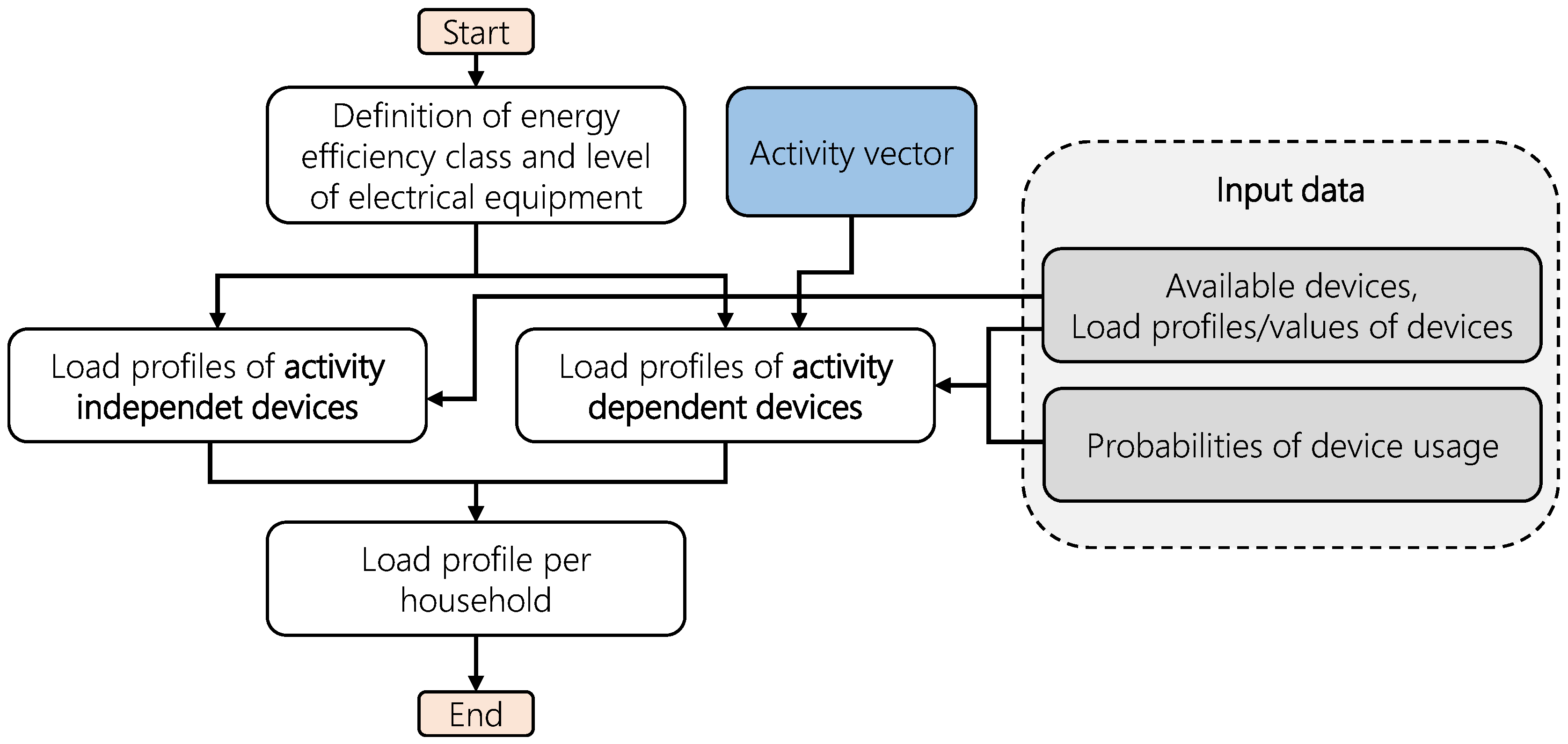
For generating the load profiles of the households the model iterates first over all households, and begins by creating the profiles for those devices which are always on and independent of the activities. Therefore, if the device is available due to the level of electrical equipment and the number of people, a load profile according to the efficiency class is randomly selected.

Second, for all other devices a load profile, or alternatively a base load value and a noise value, are chosen with regard to the efficiency class per device. Next, the activity profiles of all household members are summed up for all people present at home. This results in a matrix including all time steps of the simulation and the number of people who are performing different activities at home. Using this information, the matching of activities and usage of electric devices starts. Figure 3 gives an overview of the whole process.

During the iteration over all time steps, the algorithm checks if there is a change in the activities of the inhabitants. If there is a change, the relevant devices for this activity are taken into account. Depending on the type of activity, devices are either directly linked to the activities, e.g., watching television, or there are probabilities that devices are used. Cooking is an excellent example of this, as the usage of several devices for the same activity is possible. The following devices have possibilities that can vary over the day: stoves, ovens, kettles, microwaves, toasters or coffee machines. Assuming that the agents cook more extensively on Sundays at noon, the switch-on probabilities for kitchen appliances (stove, oven) are increased by 30% during this period. Since there is a lack of data, these possibilities were assumed as constant for the other devices and adjusted during the development of the model. So depending on coincidence, none or multiple devices are in use. To avoid unrealistic behavior, e.g., that the oven, which could be used for meal preparation as well as for baking is not used twice at the same time, an additional restriction for this device is added. So if the oven is in use for baking, it cannot be used for cooking at the same time.

Next is the differentiation between activities with direct and indirect dependencies on electricity consumption. For direct dependencies, the load profile is selected for the whole time of the activity and also ends with the activity. In contrast, load profiles of indirectly dependent devices also start with activity but continue until the selected process is stopped. For example, a washing machine is not stopped after the activity doing the laundry is over, but after the chosen program of the washing machine is finished.

As mentioned at the beginning of this chapter, lighting is modeled in a different manner. Basically, there are two different types of lighting. First, activity-independent lighting, which corresponds to the number of people who are at home and awake. Second, activity-dependent lighting, which corresponds to the activities of the inhabitants. Therefore each activity is linked with power for lighting, which depends also on the efficiency class of the household. Additionally, the global irradiation by the sun is taken into account to decide if the lighting is in use or not. Therefore for each household, an individual threshold value of irradiation is determined, below which lighting is turned on. The value of the threshold is chosen randomly for each household with a Gaussian distribution around the mean of 50 W/m² with a standard deviation of 10 W/m². If the global irradiation is below this threshold value, the light is switched on. If the value is above the threshold the lighting is reduced to a value between 0–7% with a uniform distributed random number, to model that some lights might be turned on during the day even though it is bright outside. The mentioned numbers result from different sensitivities that were done during the development process of the model.

Neglected devices e.g., mobile phones, printers, electric toothbrushes, further kitchen appliances etc. are taken into account by a constant load. Per consumption level and agent 6 W are assumed. In addition, for some appliances, such as microwave, television, stereo, etc. standby loads are implemented. These vary between 1 and 2 W and only have an effect if the corresponding devices are switched off.

After this process is finished all load profiles of the components are summed up to a household load profile. Electrical load profiles of the circulation pumps for heating and hot water were also added to this household load profile. The pump profiles were modeled with regard to heating demand, as described in [34]. See [23] for a more detailed explanation. At this step, the load profiles of the components and devices were also allocated to the three phases of the electricity system.

The described process is carried out in every household.

2.4. Mobility Model

The first steps of the mobility model, linking activities with locations, are actually implemented within the activity model because of their retroactive effect on the activity vector. Therefore, the mobility model of this work contains only the modal split and the allocation of distances and consumptions to the journeys made by car.

Even though the ZVE contains durations of the activities related travel, it includes neither distances for these journeys nor information about the modal split. Therefore, the mobility model is based on the nationwide survey MiD which researches the travel behavior of households in Germany. The study is carried out every five years on behalf of the Federal Ministry of Transport and Digital Infrastructure. The central aim of the MiD is to obtain reliable and representative information on the day-to-day travel of individuals and households. This work uses the version from 2017. The study consists of seven partial data sets. Only the data sets for individuals and journeys were used for the model. The data set for individuals contains information about the size of the municipality a person lives in. Information on the purpose, type of transport, duration, and distance of a journey is provided by the data set for journeys.

The data is filtered based on the criteria shown in

Table 6. Criteria to filter the MiD data.

Criteria	Symbol	Distinctions
Type of journey	/	Commute, other journey
By car	/	Journey is covered by car
Number of cars	$n_{\mathrm{car}}$	Number of cars the household owns
Distance	/	Distance of a journey
Speed	/	Average speed of a journey
Travel time	$T_{\mathrm{T}}$	Clustered into 11 time intervals: $0<t_1\le$ 10 min, 10 min $<t_2\le$ 20 min, …, $t_{11}>100$ min
City category	$CC$	Four categories equal to the input data Table A1

. Some journeys with unrealistic speeds are removed beforehand. The results of the data preparation process are several matrices containing probability distributions. For this, a similar approach as in Equations (1) and (2) is used. To calculate the already mentioned distribution of the duration for the activity commuting, the data set is filtered to extract all commutes. Afterwards, the probability matrix is calculated out of the remaining data by using the criteria traveling time $T_{\mathrm{T}}$ and city category $CC$. The modal split is determined separately for commuting and other travel. Therefore the criteria are T, city category $CC$ and number of cars $n_{\mathrm{car}}$.

The distances are not assigned over probabilities. A matrix containing average distances depending on city category and travel time is determined. For the distances of other journeys, a deterministic approach is chosen. The journeys are clustered based on the criteria travel time and city category. The speeds of the resulting clusters are saved so that the model can deterministically pick a random one. The distance is then calculated by using the duration of the journey and the randomly picked speed.

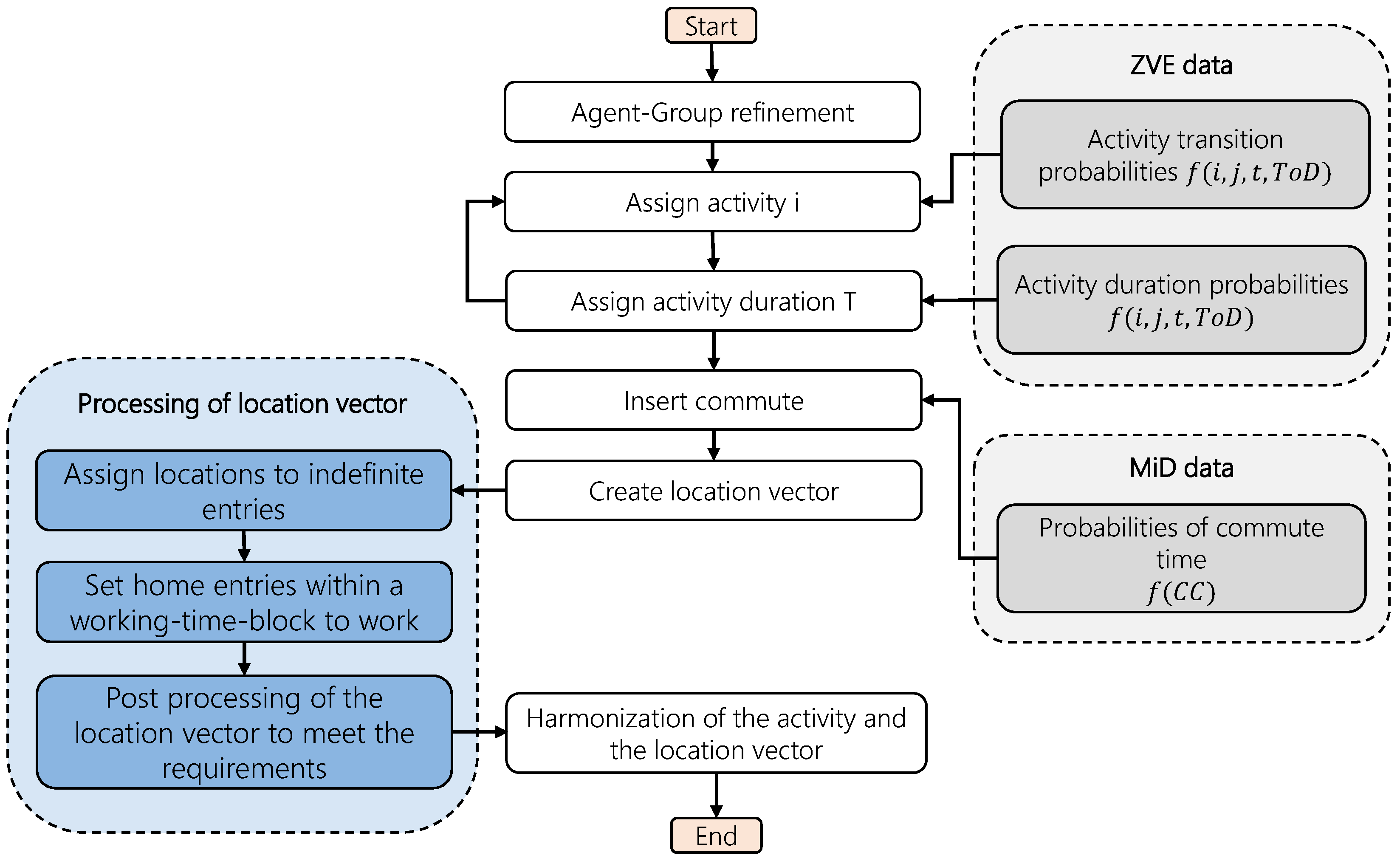
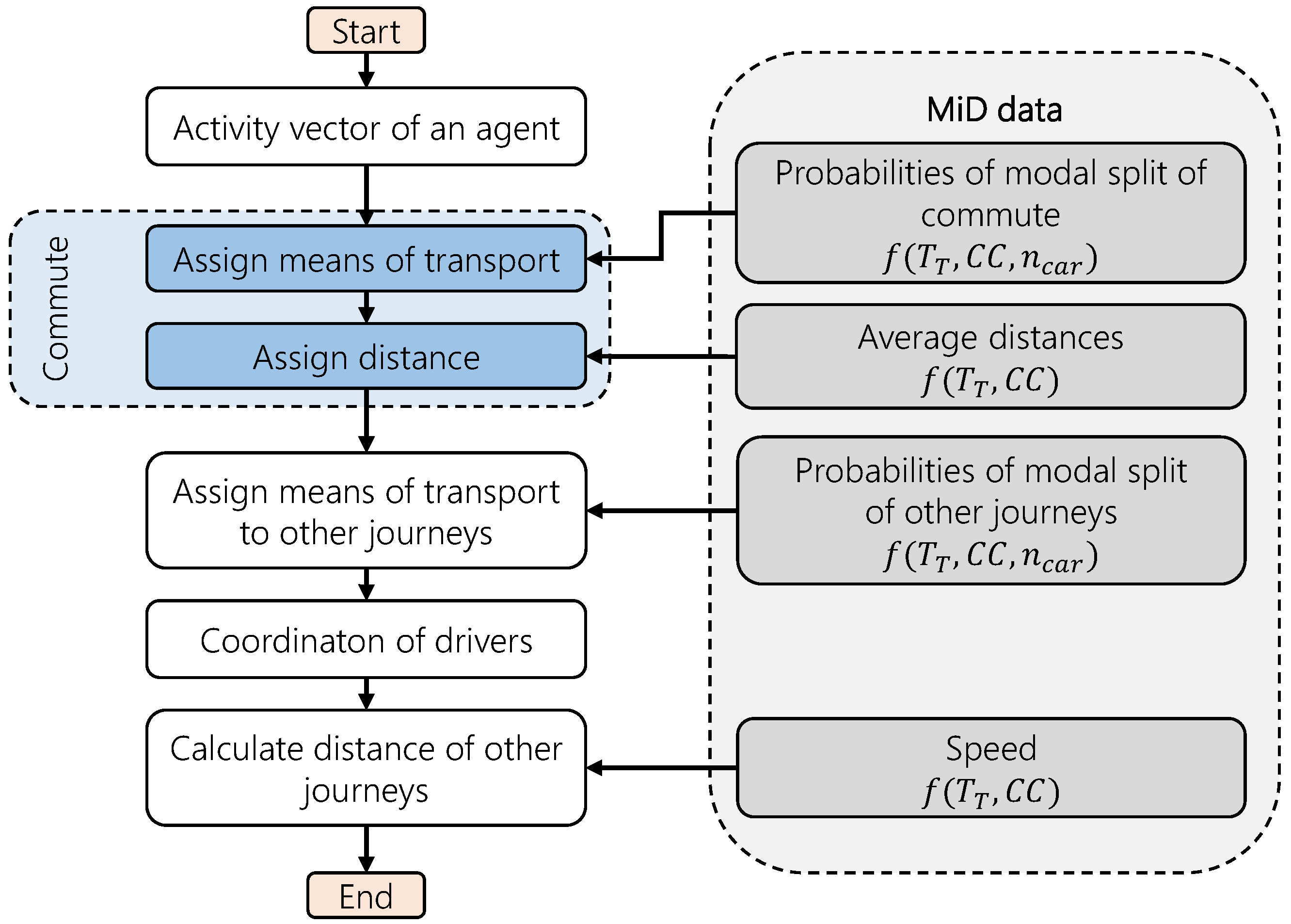
Figure 4 shows a simplified flowchart of the mobility model. The model iterates through every agent of the settlement. In the first step, the model assigns the agent a means of transport and a distance for the commute. The distance is determined by using the average distances out of the data set. The decision on the choice of transport mode is based on the probabilities of the modal split for commuting. Thus, it depends on the travel time $T_{\mathrm{T}}$, city category $CC$ and the number of cars $n_{\mathrm{car}}$ the household owns. Afterwards, the model iterates through the location vector to find every journey (commute, other journey) of the agent. For the other journeys, the modal split probabilities based on the MiD are used to decide if the trip is made by car. The information on every journey made by the car is extracted to a logbook table. The logbook contains the time step and location where every drive begins and ends. If a household has two agents who are authorized to drive but only one vehicle, the logbooks must be harmonized. Therefore, the agent with the higher travel time within the regarded time range is prioritized. The prioritized agent may always use the car. The other agent may only use the car if the prioritized agent is not disturbed by it. Afterward, the distance of every journey within the logbook is determined. As mentioned before, a deterministic approach is used for this. The model selects a real speed from the MiD-data with the same city category and travel time and calculates the distance of the journey. Exceptions are drives from home to another location and back again. For those cases, the same distance is selected for outward and return journeys. In the last step, each drive is assigned to an electrical consumption in kWh. A simple consumption model based on measured values out of [35] is used for this purpose. In this reference, the consumption of electric vehicles was determined as a function of average speed, outside temperature, and vehicle class. The model interpolates a suitable consumption based on the measured values as a function of the three influencing variables. The electrical consumption of each drive is stored in the logbook of the vehicle. The results of the mobility generator are logbooks and mobility profiles of every car within the settlement.

3. Results and Discussion

The following chapter gives an overview of the resulting activity, load, and mobility profiles from the described model. Since the focus of this paper is on the generation of the activities, the resulting electrical loads, and the corresponding mobility demand of the modeled agents, a detailed explanation of the thermal model is not shown in this paper. For the other models, the results are shown and compared to literature values and similar models.

The validation of the activity and the electric model is based on one simulation for 300 houses with 940 Households. Therefore, representative distributions for Germany based on [23] are assumed for the input parameters on household and building levels. The input parameters were already described in Section 2. A whole year is simulated. Concerning activities and electrical behavior, the city category only affects the duration of the commute. The influence is therefore considered negligible and the city category is assumed to be one, i.e., small cities with less than 20,000 inhabitants. The chosen distribution for the input parameters is given in Table A1. The input parameters described in Section 2 are defined based on distributions representative for Germany [36,37]. Thus, a representative German settlement is created. These distributions originate from the already mentioned study ZVE [21] and a population, building, and housing census of the statistical offices of Germany [38]. The values are included in Table A1. Exceptions are the distributions of the number of households within a building, the living space, and the specific heating demand. Those depend on the building type. Therefore, a detailed presentation is omitted at this point. The description of the used methodology to reproduce the distribution for these parameters can be found in [23].

To validate the mobility model, a simulation is carried out for each of the four city categories. In contrast to the first simulation, only 107 buildings with 357 households are simulated. Each simulation uses the same distributions already used in the first simulation and representative for Germany. One vehicle is assigned to each household. Thus, only the variable city category is varied. This allows a clear validation of the sensitivity of the city category.

3.1. Activitiy Model

This subsection describes the results of the activity model. The main result of this model is an activity profile that contains an activity for every agent and time step within the simulated settlement and time range.

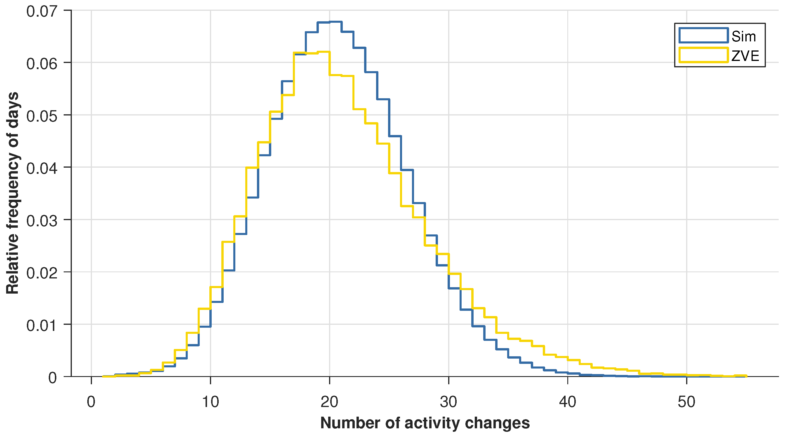
To validate the results, the average characteristics of all agents within the simulated settlement are considered. Figure 5 shows the frequency distribution for the number of activity changes. The distribution of the simulated agents is compared with the distribution of individuals from the ZVE data. The similar shape of the curves clarifies that the synthetic activity profiles cover almost the entire spectrum of the ZVE profiles. There are a few days with very few or very many changes. The relative frequency of days in the range of 0 to 18 activity changes is very similar. After that range, the distributions are slightly shifted. The ZVE distribution reaches its maximum at 19 activity changes, while the simulation reaches its maximum at 20 changes. The range with many changes is underrepresented by the simulation. Overall, the synthetic distribution can be described as slightly compressed compared to the ZVE curve. The average activity changes per day are 21 in both cases. The consistency is accepted as sufficient.

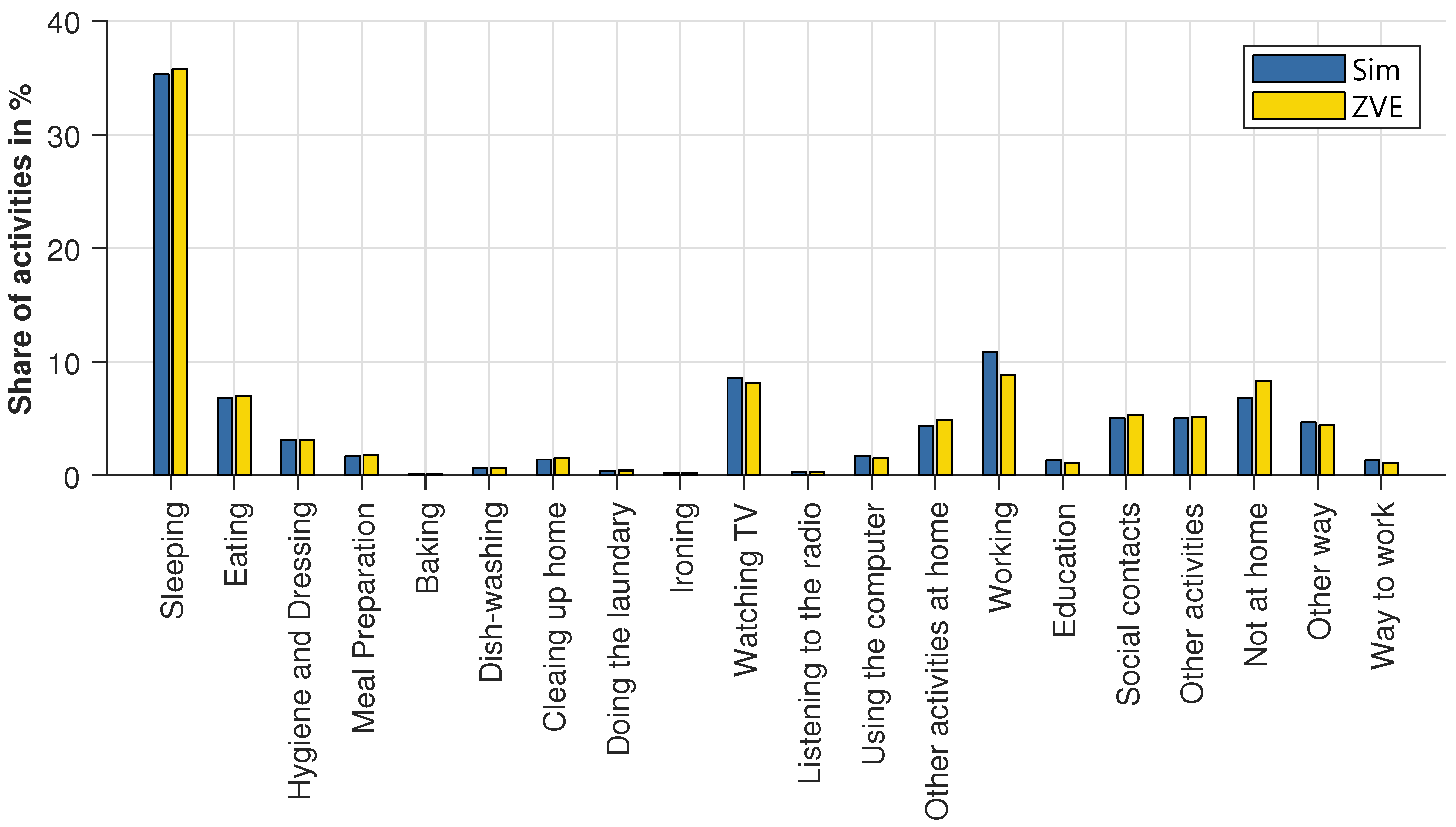
The annual percentage of activities is compared in Figure 6. Most of the activities fit very well. The absolute deviation for almost all activities is significantly below 1%. However, the activities working and not at home have a higher deviation from the ZVE data. By assuming that activities located at home are prohibited during the working-time-blocks, the activity profiles were subsequently edited. This explains the higher proportion of the activity working (absolute deviation is 2%). However, this percentage is then no longer available for the activities clearly located at home, e.g., sleeping. The insertion of missing journeys and the extension of return journeys are carried out at the expense of the activities not at home. This explains the 1.5% lower share of the activities not at home. The activities related to travel fit very well, although the commute was completely inserted afterwards. Excepting the activities working and not at home, it can be concluded that the activity generator reproduces the activities of the original data over the whole year very well. The significant deviations are caused by the restrictions necessary to generate a plausible mobility profile and are therefore tolerated. The remaining deviations are negligible.

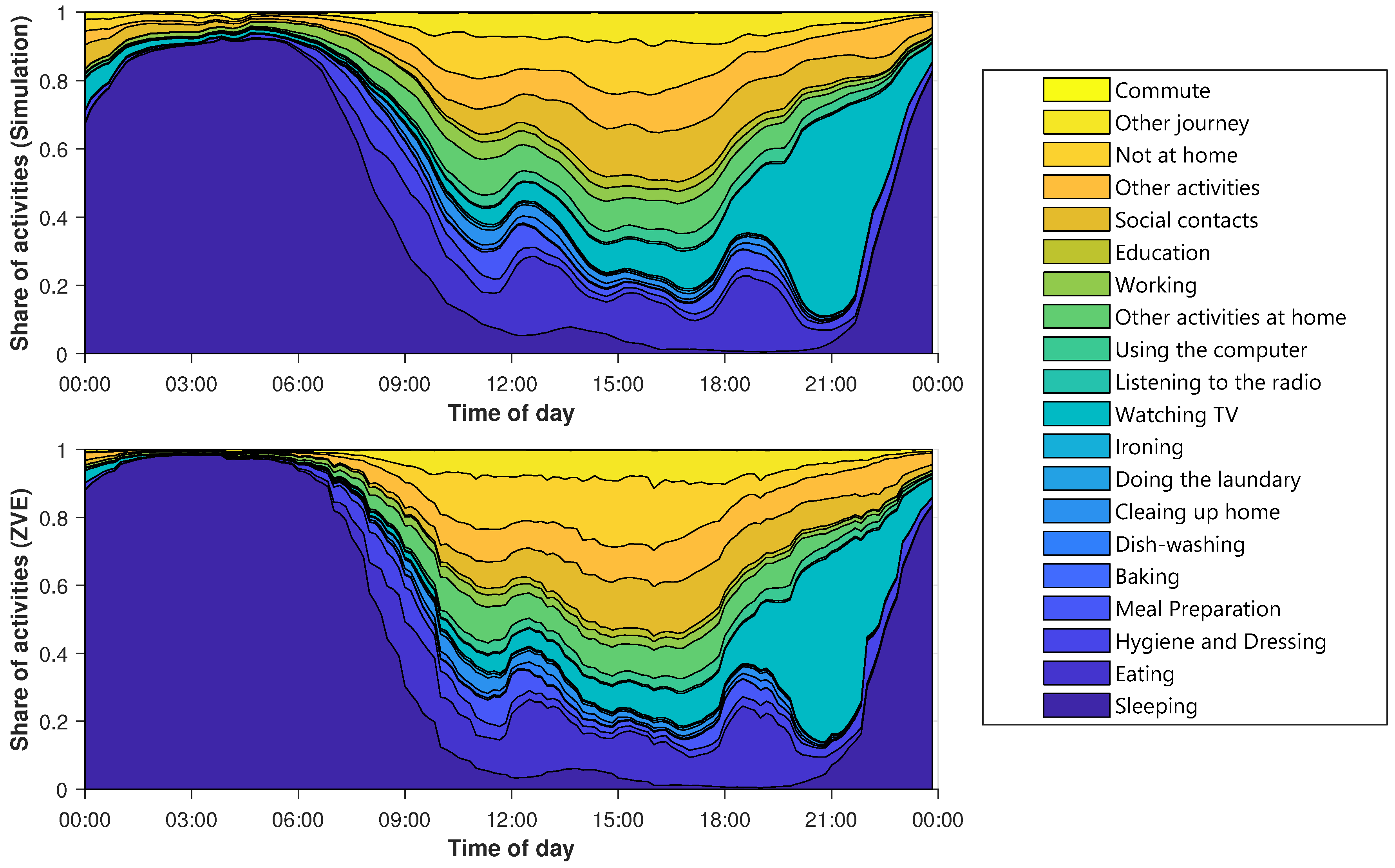
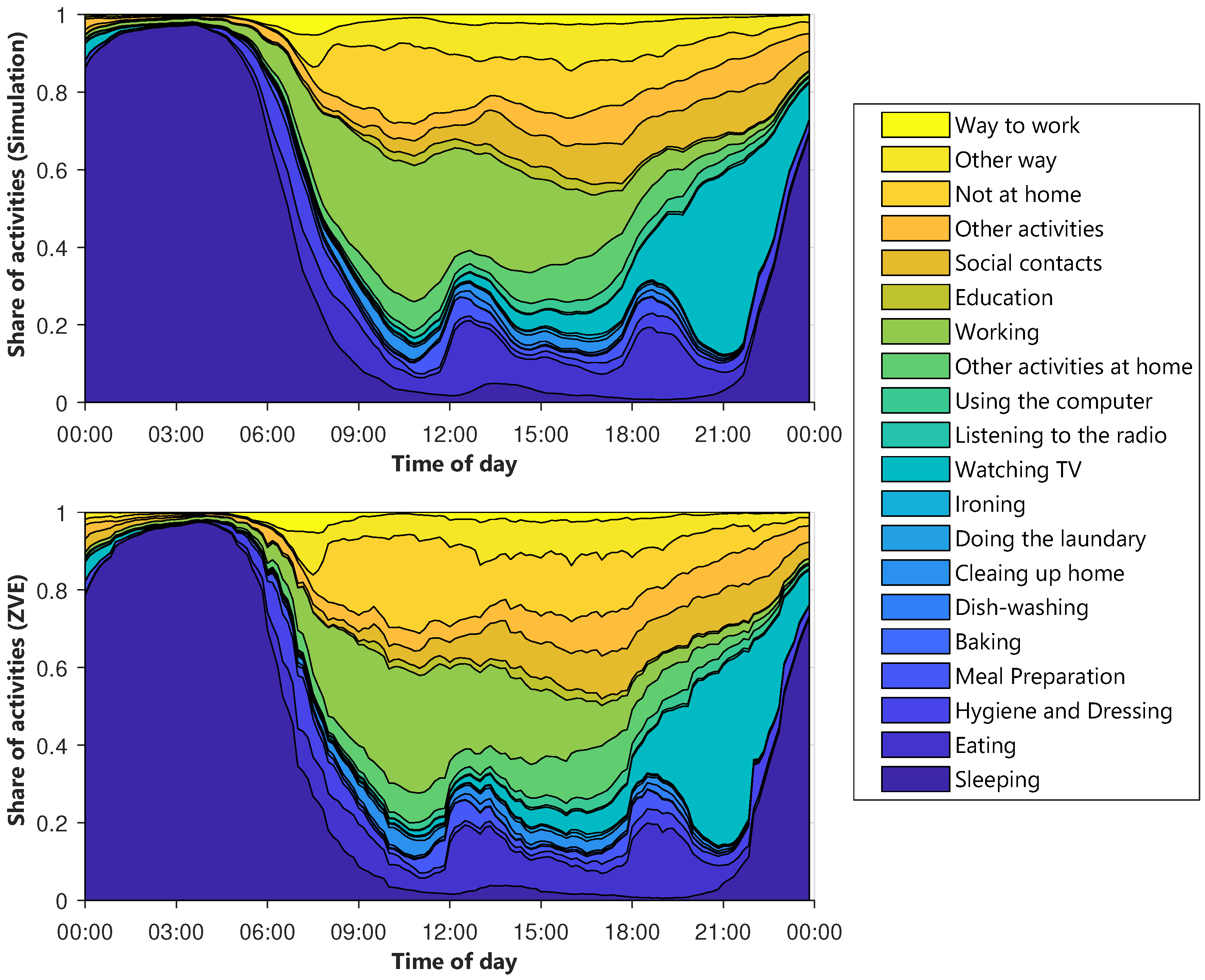
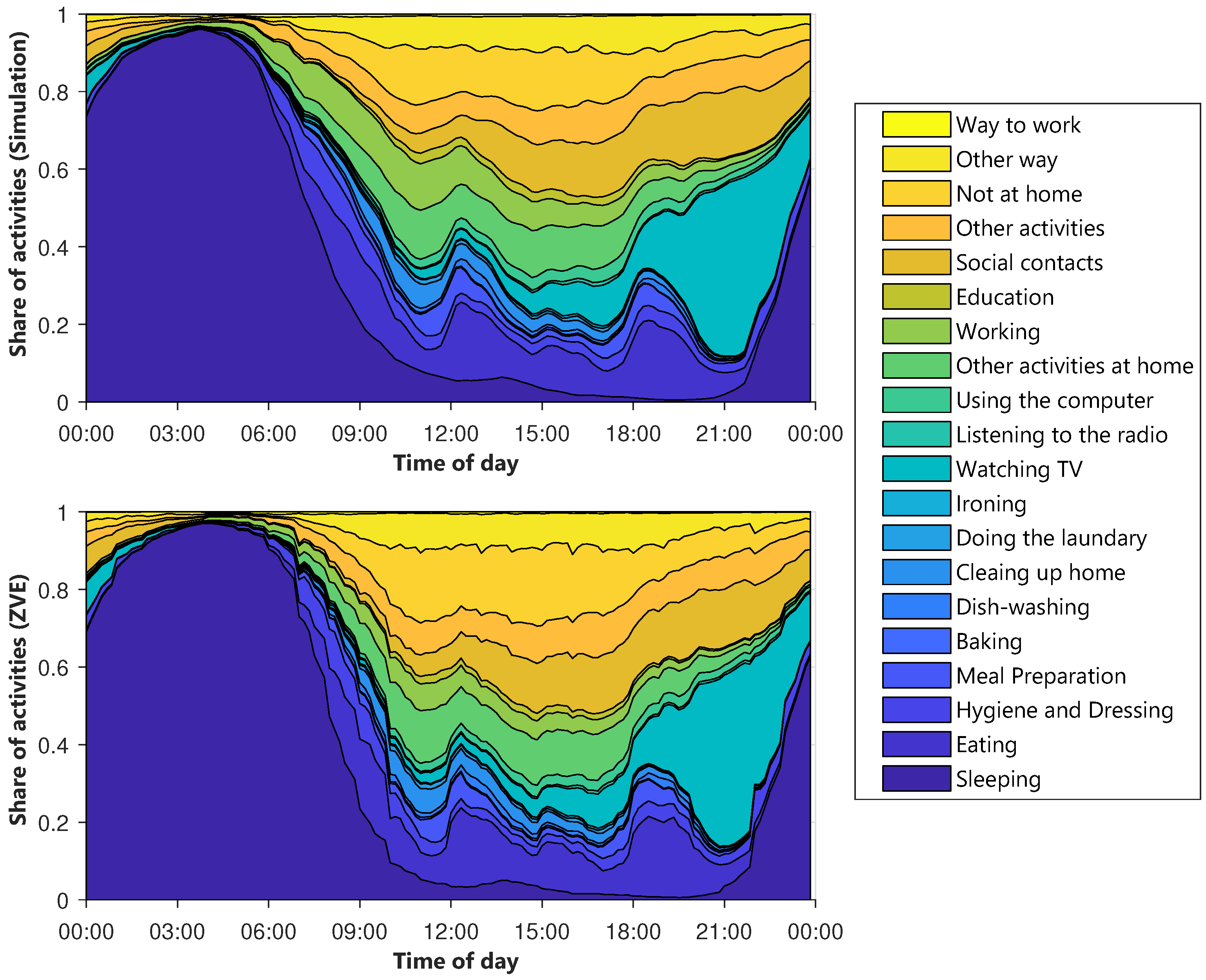
Besides the percentage of activities, it is also particularly important when the activities occur. Later on, this will have a major influence on the shape of the electric load profiles. Therefore, the average layered course of the activities is examined in Figure 7. The y-axis shows the percentage of agents that perform an activity at a given time. The x-axis contains the time of day. The different types of days are considered separately. Figure 7 shows the diagram for Sunday.

The diagrams of the other types of days are shown in Figure A1, Figure A2 and Figure A3. The top diagram depicts the synthetic activity profiles, while a corresponding diagram for the ZVE-data is plotted below. Immediately noticeable is the smoothing of the synthetic curves. It can be explained by the sample size, because the generated data set contains significantly more day profiles than the ZVE-data set. The comparison confirms the deviations already noted in Figure 6. Not at home is slightly under-, and working is slightly overestimated. However, the temporal progressions match very well.

3.2. Thermal Load Model

The thermal model is not the main scope of this paper. Therefore only some key results are shown in this chapter. First, the results for the heating demand are shown and described.

3.3. Electric Load Model

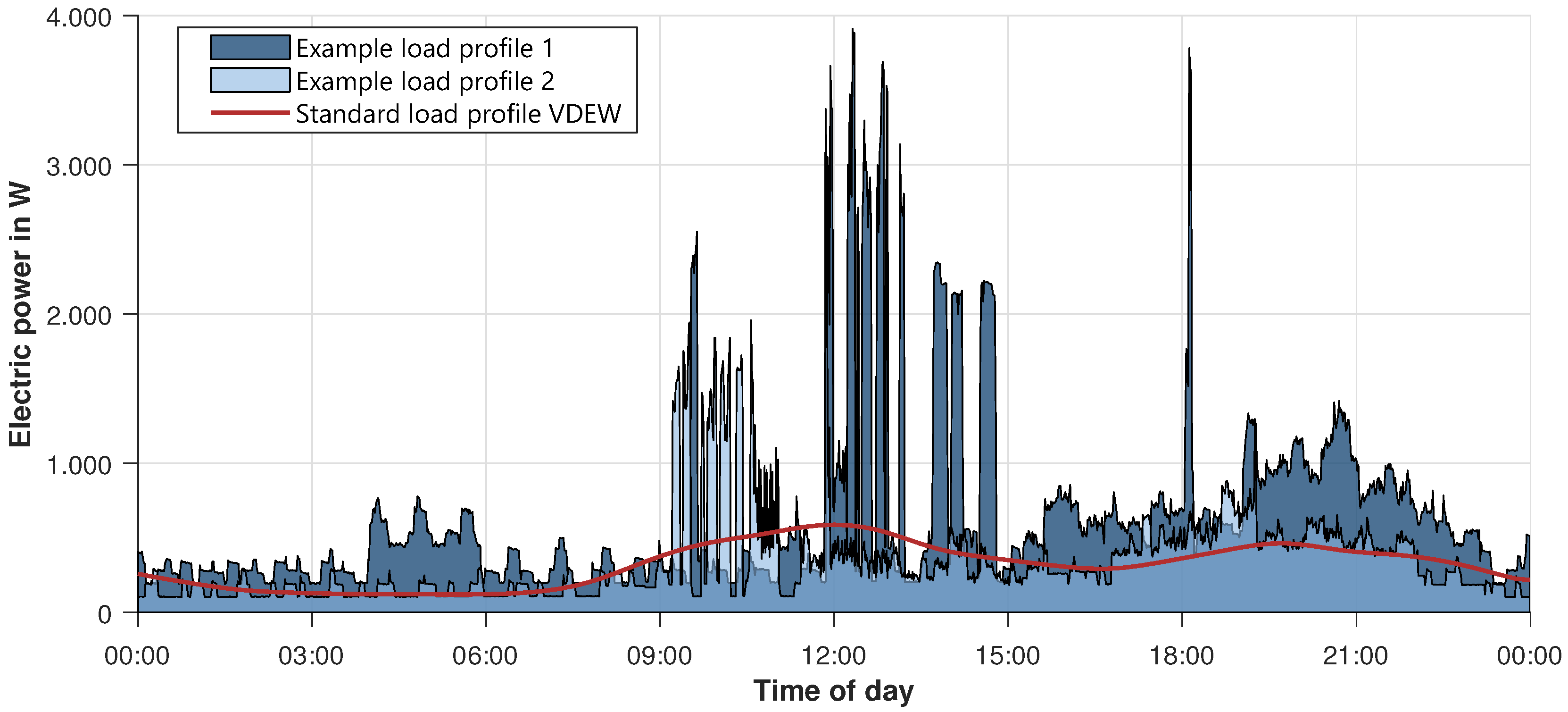
In this section, the results of the electric load model are presented and validated. Different scopes are necessary to fulfill all requirements regarding a realistic load profile for load flow calculations. First, the energy consumption of different households and devices is analyzed. Second, focus is placed upon the shape of an average power profile. Finally, the occurrence of simultaneous power peaks, which are very important for simulations and gradients of the profiles, are discussed. To give an overview of how different a single profile is compared to an SLP, see Figure 8. Figure 8 makes it clear that a single profile has much higher peaks, e.g., profile 1 at around 4 a.m., but that there are times where there is almost no energy demand. This is also the reason why the SLP is not suitable for a detailed simulation of less than around 150 households [6].

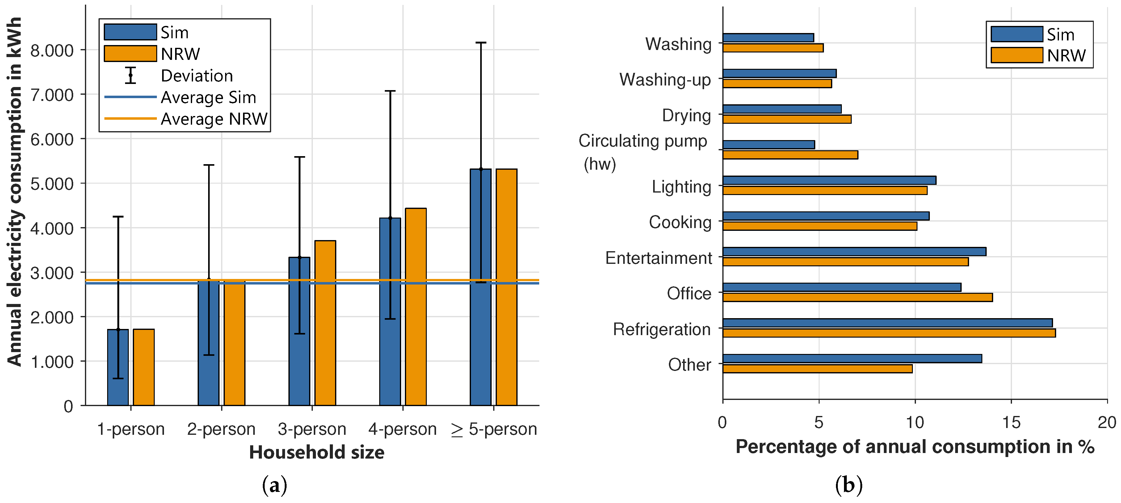
After the general overview, one key indicator of the model quality is the energy consumption per household (HH).

Table 7. Energy consumption per household in Germany in literature and simulation.

Source	1-P HH	2-P HH	3-P HH	4-P HH	5-P HH	Year
EA.NRW [39]	1714	2812	3704	4432	5317	2015
Stromspiegel, SFH [40]	2300	3000	3600	4000	5000	2019
Stromspiegel, MFH [40]	1500	2100	2600	3000	3600	2019
Destatis [41]	2005	3205	4856			2017
Simulation	1708	2835	3330	4215	5315	-

gives an overview of the annual energy consumption for different households from the literature. The first study [39] was conducted by the energy agency North Rhine-Westphalia in 2015 and included 522,000 households. In addition to the total consumption, the shares of different devices were also analyzed. Regarding this study, the consumption ranged from 1714 kWh for one person to 5317 kWh for five persons. In other studies, the range was a bit smaller (1500 to 5000 kWh) [40] but a distinction was made between single and multi-family houses. For this study, more than 226,000 households were analyzed. The last and most recent study [41] from Destatis only provides data for one- and two-person households, and households with more than two persons. All values are for households without electrical heating since this is not part of the described model. Finally, the resulting energy demand per household type of simulation is also added to the table.

For a better understanding, the results of the simulation and [39] are visualized in Figure 9a. On the left side, the different household sizes and the overall average, resulting from the modeled settlement, is shown. Here the overall energy consumption only deviates by 2.5%. In this scenario, households with one, two, or more than four persons have a slightly higher, and the other households a slightly lower energy demand than in [39]. The black lines also show a large variation between households in the same group. For example, in the simulation demand of a single-person household varies from 608 to 4247 kWh, which shows that the model produces realistic results. On the right side of Figure 9b, a percentage of annual energy consumption per device group of the simulation and the chosen study is shown. Overall, the figure indicates a good behavior of the model, even though there are some deviations of a maximum of 4% per group. Most obvious is the deviation at “other”, which is higher in the simulation. This group also includes the additional load per agent, which represents devices like mobile phones, tablets, or printers, in the model. This is also an explanation of why the “office” is slightly underrepresented. The circulating pumps in our model are underestimated, but this is part of the thermal model, which is not a focus of this paper. In total, the energy demand per household type as well as the allocation to different device groups is very close to the results of [39].

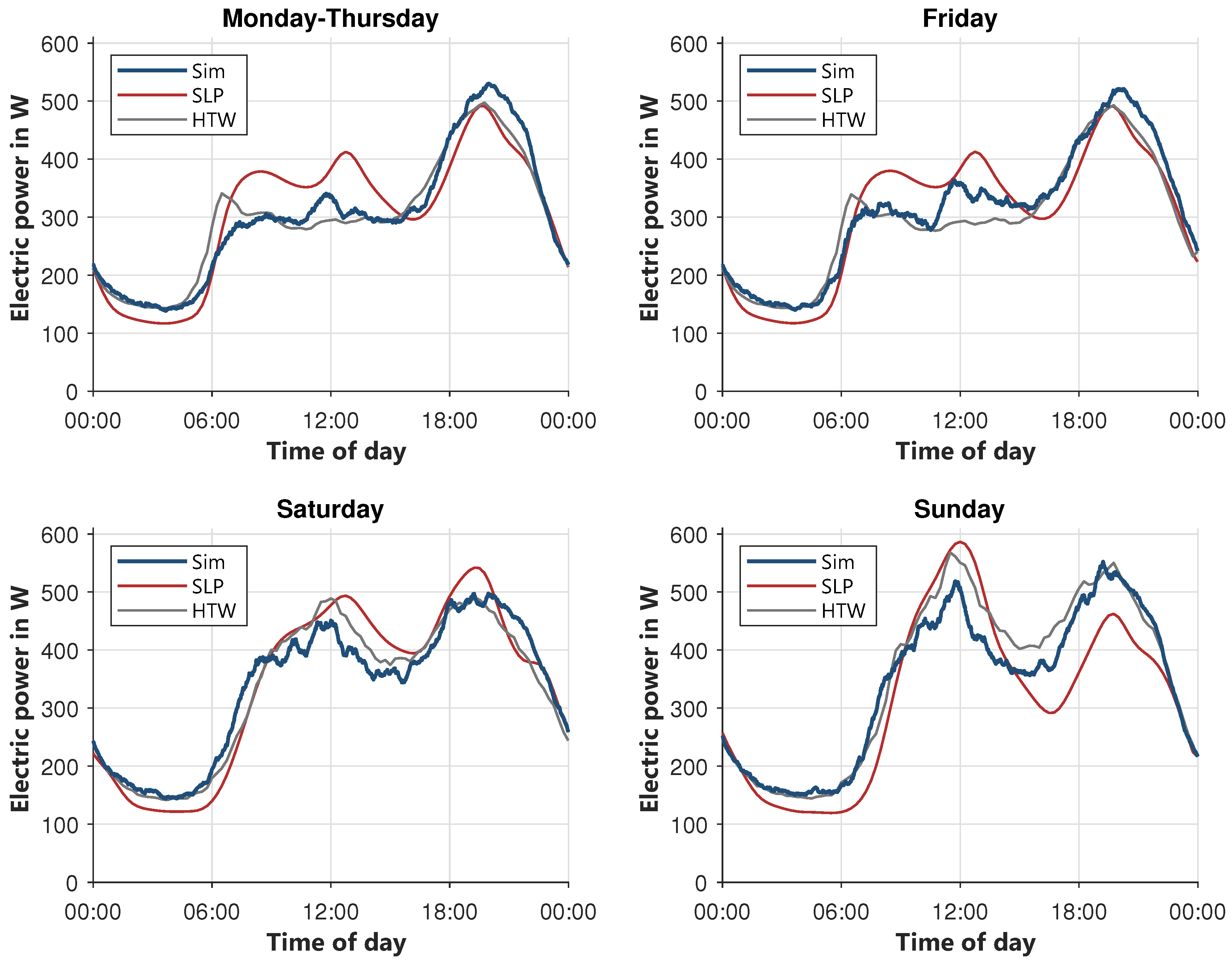
Besides the overall energy consumption and the usage of different devices, the resulting profile of the households is fundamental for the usage in a load flow calculation model. To validate the model, two different sources are used. First is the SLP, which is used for billing and procurement, and dates from the year 1999 [5]. In contrast to that, the University of applied sciences Berlin (HTW) describes 74 representative load profiles with a temporal resolution of one second [42]. In Figure 10 the two references and the modeled profile are shown for four types of days (Monday–Thursday, Friday, Saturday and Sunday) since these types of days are different regarding the user behavior. Unfortunately, the SLP does not distinguish between Monday–Thursday and Friday. In general, all profiles have a similar shape, with the lowest load in the early morning hours. Afterwards, at around 6 am, the load starts to increase with a peak at noon, which is higher during the weekend, since there are more people cooking at home. This peak is mostly followed by a dip in the afternoon before the load reaches its peak in the evening at around 7 p.m. For comparison and illustration purposes in the following figures, all load profiles were aggregated to 15 min resolution.

Comparing the two reference profiles shows that there is not a clear “right” profile. The biggest difference occurs on weekdays during noon, where there is a peak in the SLP but none in the HTW profile. The potential reasons for this difference are manifold, starting with the fact that the SLP dates from 1999, whereas the HTW profiles were measured in 2010 and are therefore perhaps closer to contemporary usage patterns. On the other hand, the SLP is still in use in the accounting processes of grid management. For these types of days, the modeled profile largely falls between the reference profiles, and somewhat closer to HTW. Exceptions are the flatter slope in the morning hours, resulting in a lower morning load, and the comparatively higher evening peak. On Fridays, the modeled profile has a slightly higher demand in the afternoon than on the other weekdays. On Saturdays, the modeled profile has a lower peak at noon, but a higher load in the night hours starting from 8 pm. Overall, the simulated profile is quite close to the reference profiles for Saturdays. On the last subfigure, Sunday, the peak at noon is underestimated, in contrast to the other profiles.

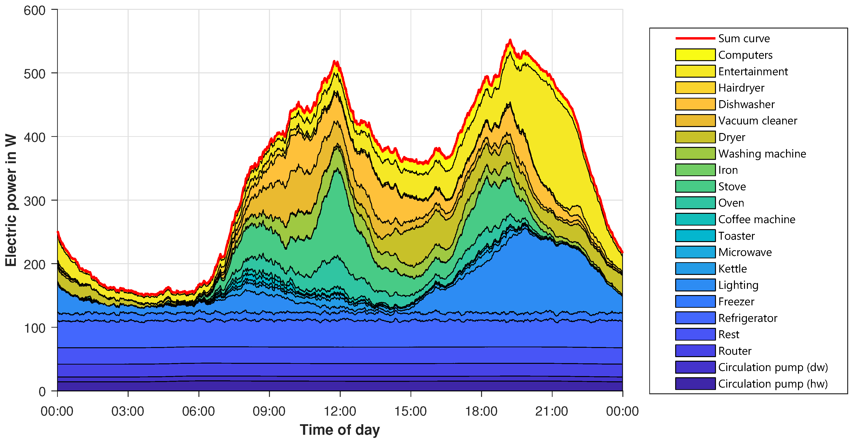
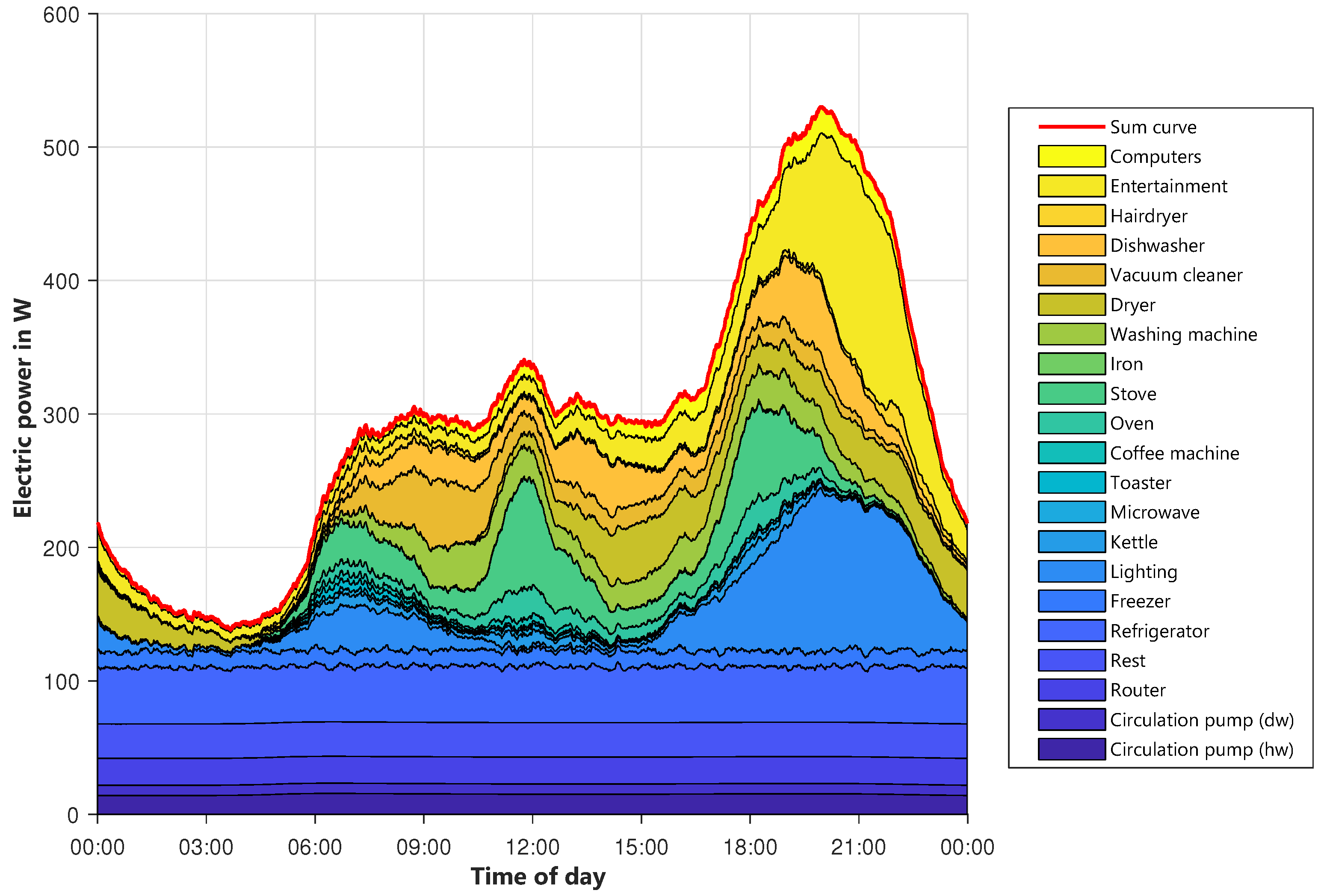
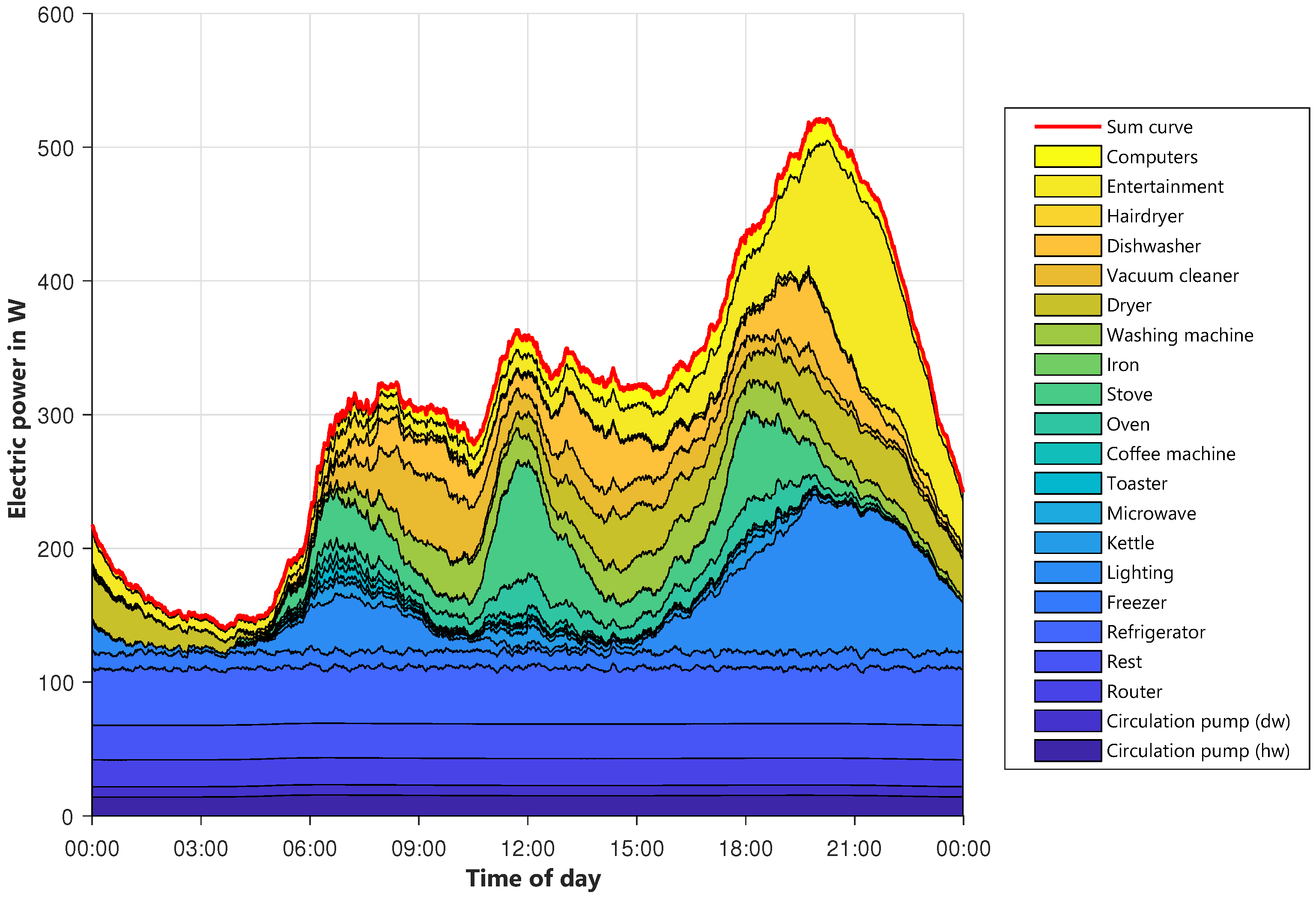
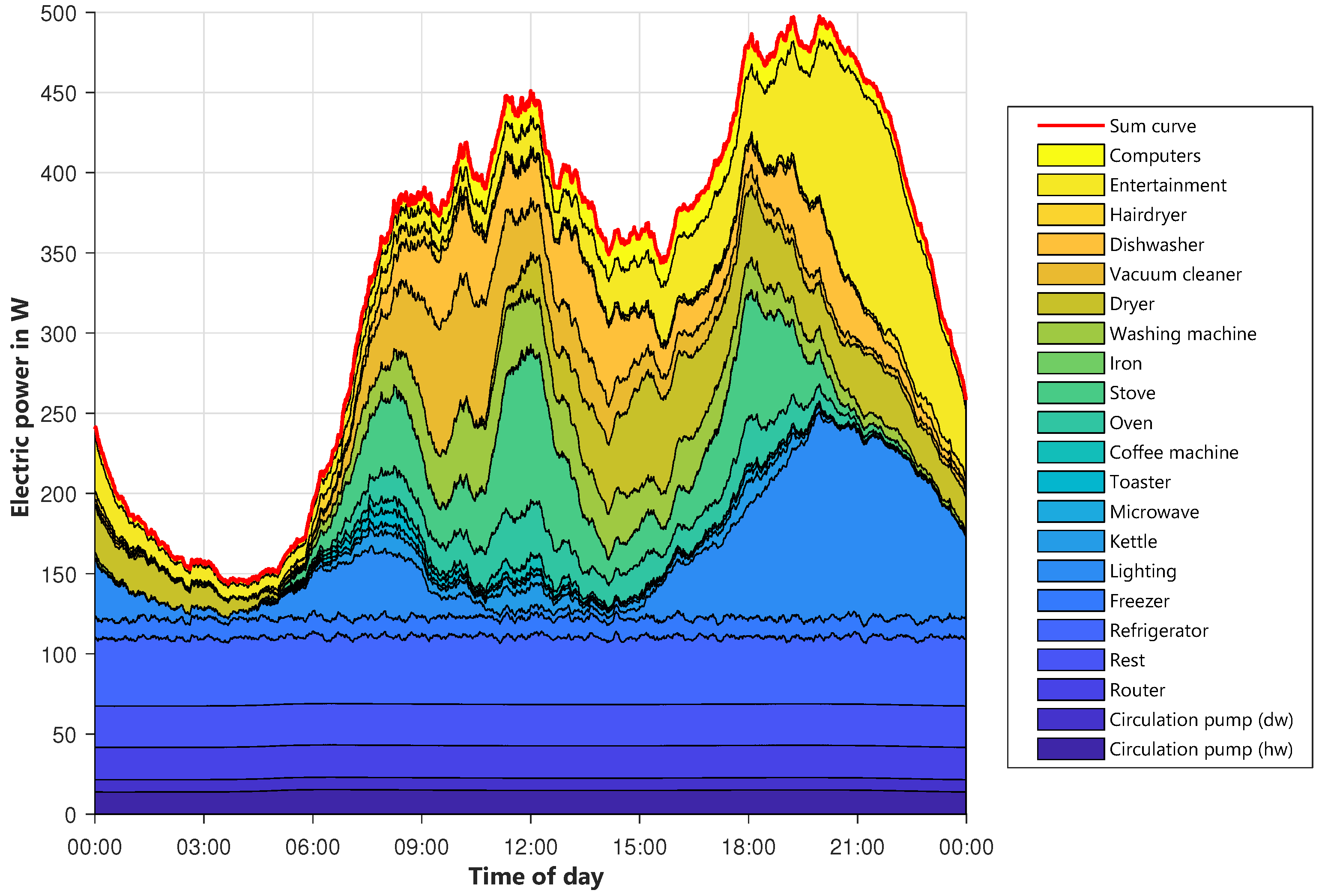
To examine the modeled profile in more detail, Figure 11 shows the allocation of the power to different device groups. Starting from the bottom, the base loads like circulating pumps, routers, and so on, are displayed. The first bigger load forming the shape of the profile is lighting (light blue), which is mostly on in the morning and evening hours. Cooking equipment also contributes to the evening peak, alongside higher usage of entertainment equipment, like televisions or stereos, and lighting. On the whole, the modeled profile is similar to the reference ones. The shape fits quite well even though there are some smaller deviations. In total, the modeled profiles are closer to the newer HTW profile than to the SLP, which is quite old. Since there is no right or wrong behavior for this shape, and also taking into account that the behavior of people has changed over years since 1999, the result seems to be appropriate for the planned usage.

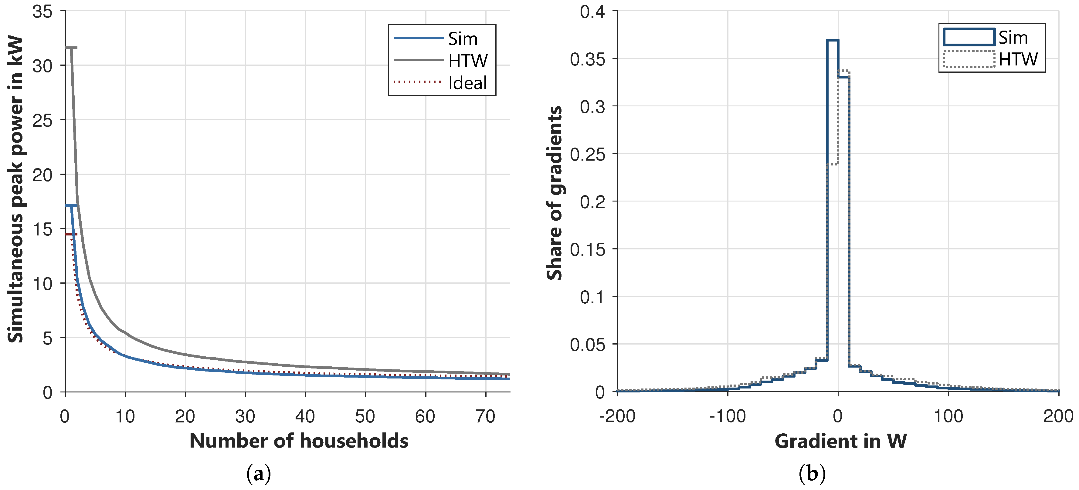
The last two important indicators which are compared are the occurring simultaneous peak power and the resulting gradients from one minute to the other. The maximal simultaneous power of households describes the maximum concurrent peak load for a number of households. Since not all houses use their maximal power at the same time, this value decreases rapidly with the number of households. If there is only one household connected to the grid, the grid must be able to deal with the maximum power of this household. If there are more houses connected, the maximum occurring power $s\left(n_{HH}\right)$ at a time is lower than the sum of the individual peak powers. To calculate this value, n profiles were summed up and divided by the number of households, as in Equation (3). This process was carried out 10,000 times and the maximum of each combination was saved. From these 10,000 results, the 95% quantile was used to calculate a realistic value. [43] This procedure was performed for the results of the described model and also for the load profiles modeled by [42]. In literature, an approximation for the simultaneity factor is often used [43,44]. Equation (4) calculates the simultaneity factor, which describes which percentage of the individual maxima are occurring at the same time at a given number of households. To get the resulting power per household, this value must be multiplied with the peak power per household. Within the DIN 18015 [45] this value is estimated to be 14.5 kW for one house without electric heating or water preparation.

$$s\left(n_{HH}\right)=\frac{P_{HH,occ,max}\left(n_{HH}\right)}{n_{HH}}$$

(3)

$$s\left(n_{HH}\right)=0.06+(1-0.06)\times {\left(n_{HH}\right)}^{-0.75}\times P_{max}$$

(4)

The results of the simultaneous peak power are shown in Figure 12a. The results of the described model are quite close to the ideal curve calculated by using [44]. The peak power for one household is 17.1 kW instead of 14.5 kW. In contrast, the results of the data from [42] have a peak power of 31.6 kW, which is around two times as high. For all these calculations, the one-minutes values were used. The curve of all three lines is similar and is falling rapidly. At ten households, the simultaneous power of the modeled load profiles is only 3.3 kW, which is less than 20% of the overall peak. In total, this figure shows that the resulting peak powers and their simultaneous occurrence are reasonable for performing load flow calculations.

The last important indicator is the occurrence of gradients, which describes the change of power from time step to time step. Low gradients are characteristic of a very constant load profile, which typically occurs at night. High gradients indicate a strongly fluctuating load profile and occur in households mostly through switching power-intensive devices on or off. This value is very important for all control strategies since it is much easier to control a stable system than a system with high gradients. For this value, the data of [42] is again used as a benchmark. In Figure 12b the share of the gradients are shown in 10 W steps. Most of the gradients (~70%) are around ± 10 W for both data sets. The described model has more gradients −10–0 W, but slightly fewer higher gradients in the area of ±50–100 W. In total, both curves look very similar and therefore the power changes look reasonable.

To sum up the results of the electrical load model based on the modified Markov activity model, the results are validated with data from literature and other models in the fields of energy consumption per household group and energy consumption per device group. In these fields, the results look reasonable. In the next step, the average profile of many households was investigated and compared to the SLP and HTW data. Unfortunately, there is no right profile to benchmark the results. In general, the generated results are close to or between the benchmark data. Lastly, the most important indicators, the simultaneous peak power and the occurrence of gradients, were analyzed and compared to other data. Both indicators appear accurate with regard to the comparison values. Therefore, the aim of the model, the creation of electrical load profiles for different households based on the activities of the persons living in the houses, is fulfilled.

3.4. Mobility Model

This chapter validates the results of the mobility model. Important mobility parameters of the agents and the vehicles, such as the mobility rate, the kilometrage and the duration of the journey, are compared with the values given in the MiD [46]. The validation is carried out with a view to the future use of the model. The weightings specified in the MiD are taken into account. For general comparisons, the distribution of vehicles among the city categories based on the MiD data is used and the simulation results are weighted accordingly.

Table 8. Distribution of vehicles among the city categories based on MiD.

Percentage in %	City Category	Description
42.07	1	Rural region: ≤50.000 residents
20.19	2	City: from 50.000 to 450.000 residents
19.2	3	Large city: from 450.000 to 650.000 residents
18.54	4	Metropolis: ≥650.000 residents

contains the distribution for weighting the results of the different city categories based on the vehicle distribution in the MiD. With the help of the weightings, the results were combined to achieve a distribution representative for Germany.

Before considering the characteristics of the vehicles in the next step, important mobility parameters of the agents will be briefly discussed at this point. The overall values of the simulations are compared to those of the MiD [46] in the upper part of

Table 9. Average mobility parameters per day.

Parameter	Unit	MiD	Sim	MOP
Mobility rate of agents	%	85	92.3	91.3
Travel time per mobile agent	min	100	91.3	83
Number of journeys per agent	/	3.1	3.2	3.27
Number of journeys per mobile agent	/	3.7	3.5	/
Mobility rate of cars	%	59	75.6	/
Average number of drives per car	/	1.9	2.2	/
Average kilometrage per car	km	30	29.4	/
Average driving time per car	min	46	56.94	/

. If available, the related value of the mobility panel (MOP) [47] is attached. MOP is another mobility study representative for Germany. The average values are on a daily basis. The mobility rate generated by the model is, compared to the MiD, about 9% overestimated. That means too many agents are assigned to activities related to travel in the activity model. However, it is very close to the value of the MOP. The daily travel time and the number of journeys per mobile agent lay between the values of the two studies. The comparison shows that although the simulated values differ from the MOP, the studies themselves show noticeably different results. It can be stated that the simulated mobility behavior of the agents lies well between the results of the studies and is therefore assumed as valid.

The next step is to validate the mobility behavior of the vehicles. The generated mobility profiles of the cars are the main output of the mobility model. Therefore, important parameters of the mobility profiles are considered and evaluated at this point. Some important parameters are compared with those of the MiD in the lower part of Table 9. The mobility rate of simulated cars is significantly higher than in the MiD. The already discussed higher mobility rate of the agents is one reason for that. Consequently, more trips are made by car. Another major reason is the assumption, that every simulated household has only one vehicle. According to the MiD, 53% of households across Germany own one car, 21% own two and 4% own more than 2 cars. This means that the cars in the model are used by more drivers, which leads to a higher mobility rate of cars. These reasons are also responsible for the higher number of drives in the model. The average daily kilometrage of the simulated cars undercuts the MiD values slightly, even though the number of daily drives is lower and the cars are underway around 10 min more per day. As a result, the average distance per drive is underestimated by around 2 km in the simulation.

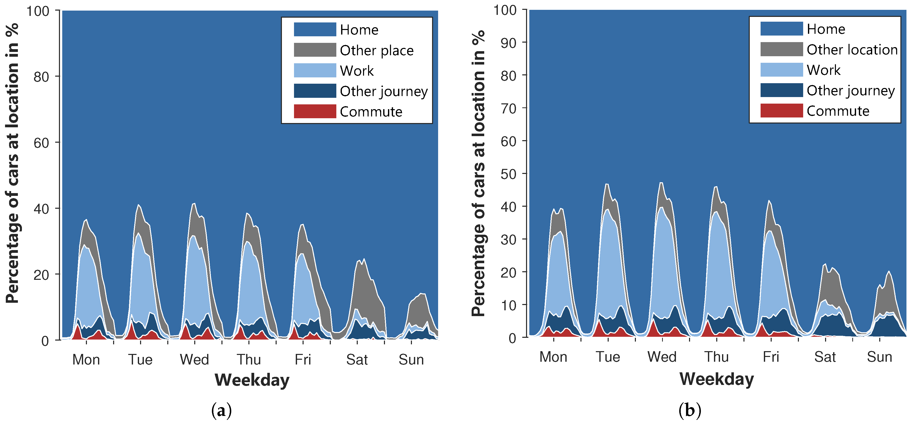
The layered percentage of vehicles at the five defined locations over the week is shown in Figure 13a for the MiD data and Figure 13b for the simulated profiles. To outline the reference course of the MiD, the information of the cars for which all routes were recorded within the study are used. As some of the necessary information is not directly contained in the MiD and the study only includes single days, some assumptions had to be made. The destinations are determined by the purpose of the journey. The places between the journeys are determined using the start- and end locations of the journeys. From the beginning of the day until the beginning of the first journey, a vehicle is located at the starting point of the first journey. Using the destination of the last journey, the location at the end of the day is determined similarly. As complete annual profiles are available for the simulated vehicles, no further assumptions are necessary to create diagram Figure 13b.

In general, a clear similarity between the two diagrams can be identified. In both diagrams, the commute occurs mainly on weekdays. On weekends, less than 1% of the cars commute to work. In both cases, most vehicles are on their way to work around 8 a.m. The peaks are in the range between 4–5%. Deviating from the MiD, the maximum of the commute on Mondays is lower than on other weekdays. At lunchtime, the proportion of commuting vehicles reaches a minimum. The minimum of the MiD is below 1%. The simulated course is in the range between 1 and 2%. The return journeys from the workplace are spread over the rest of the day and peak around 5–6 p.m. in both diagrams. The shape of the other travel on weekdays is similar, too. In the afternoon, both diagrams reach their peaks. However, the peaks of the simulation exceed those of the MiD. Accordingly, the travel time of the simulated cars is slightly overestimated, which is consistent with the findings in Table 9. Furthermore, the percentage of cars at the workplace is noticeably overestimated by the simulation even though the shape of the curves is very close and reaches its maximum around 12 p.m. Additionally, the cars of the simulation remain at the workplace longer, and more cars stay overnight. The percentage of cars at other places is slightly underestimated within the simulation. However, the differences between other places and at work balance each other out, so that the percentage of vehicles at home is relatively similar. In total, more than 53% of the simulated cars and 58% of the cars of the MiD are at home over the whole week. At the weekend, more vehicles are continuously at home. In general, it can be concluded that the locations of the vehicles over the week differ in places from those of the MiD. However, a good overall consistency is achieved.

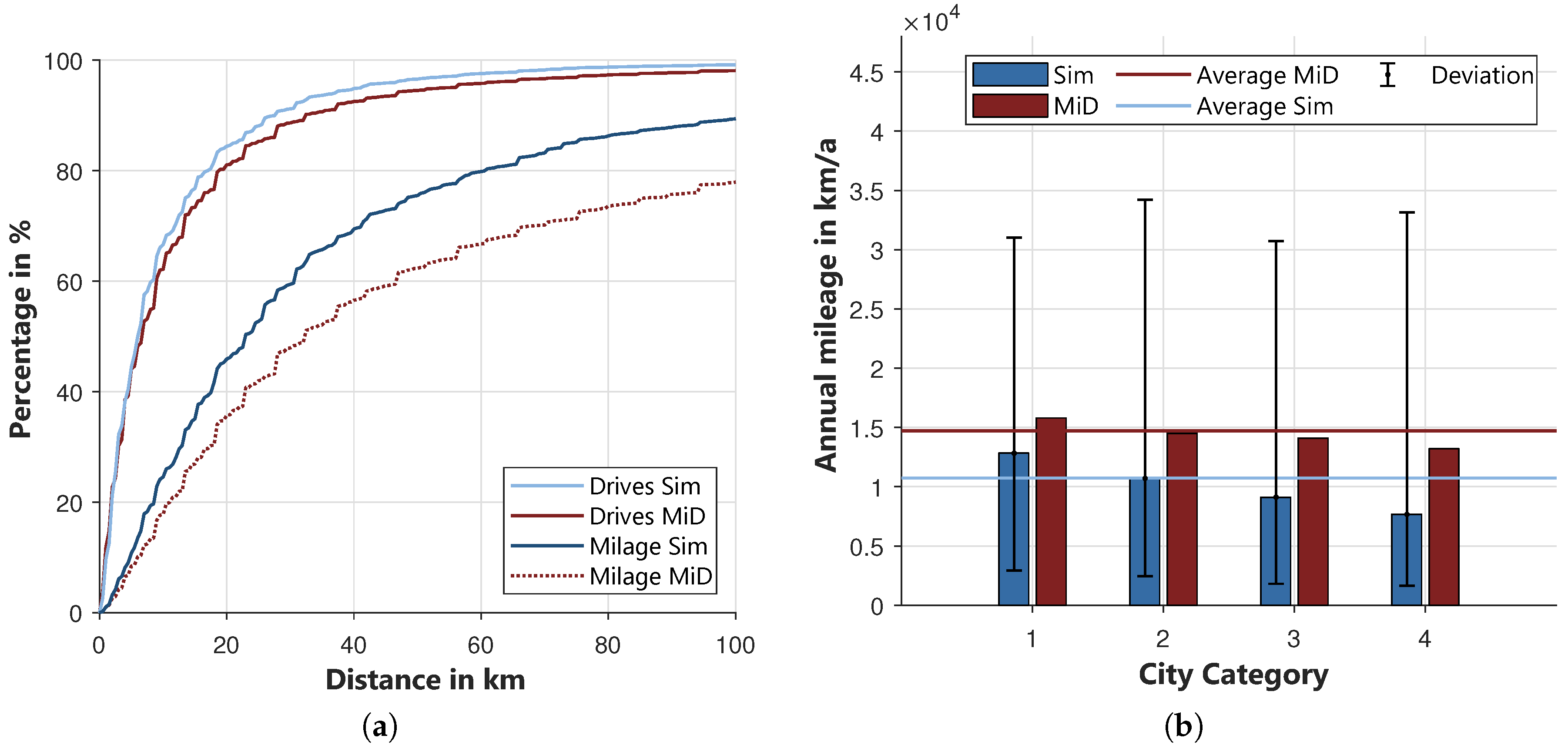
To validate the kilometrage of the cars, the percentage of drives of the total number of drives and of the total kilometrage is calculated as a function of the distance. To illustrate the share of long trips, both shares are cumulative. The resulting curves are compared to those of the MiD data within Figure 14a. The curves of the percentage of drives are very close. The simulated curve lays slightly over the curve of the MiD. This already suggests that short distances are over-, and very long distances are under-represented, because the simulated curve will reach 100% earlier. The curve of the driving performance confirms this assumption. Almost 90% of the kilometrage is achieved with drives of less than 100 km, whereas in the MiD this value is only 78%. The flattening of the simulated curve starting at 40 km indicates that trips with distances below 40 km are particularly overrepresented. This deviation is partially caused by the underrepresentation of journeys with very long durations in the ZVE. Very long drives can only be generated in the mobility model if the corresponding activities’ durations are generated in the activity model. Furthermore, to achieve a consistent mobility profile, journeys are inserted subsequently. These are assumed to have a constant duration of 10 min. Both reasons cause an overrepresentation of short distances within the model.

Figure 14b compares the average annual kilometrage of the simulated cars with the estimated kilometrage given in the MiD [46]. The four city categories are considered separately. Besides the annual values, the range in which the simulated driving performance lies is shown. It becomes clear that the model underestimates the total annual kilometrage. In the MiD, the kilometrage representative for Germany is 14,700 km, whereas the simulated kilometrage is only 10,700 km. This means that the total kilometrage is underestimated by around 4000 km. This also becomes clear when comparing the kilometrage of the individual city categories. The deviation for city category 1 is still relatively small. Just like in the MiD, the kilometrage decreases with the city category. In city categories 2 to 4, the difference is significant. The range of deviation of the simulation from the average shows that vehicles with higher kilometrage are also represented in the model. The declarations already mentioned for Figure 14a can be used at this point again. Due to the higher proportion of drives with short distances and the underrepresentation of individual drives with very long distances, the total annual kilometrage is underestimated. In [46] it is stated that in metropolitan regions the vehicle is used significantly less than in rural regions. However, the annual kilometrage of both regions is only slightly different. The reason for this is that metropolitan vehicles are used much more frequently for drives over long distances. This behavior cannot be reproduced in the model, as only the commute and the model split depend on the city category. Within the model, the duration of a journey is independent of the city category. The deviations are actually not negligible. However, it must be considered for which purposes the model is to be used, namely to investigate the electrical consumption of households. Therefore, the home charging of electric vehicles will play an important role in the future and this is to be investigated with the model. However, journeys over long distances will play a subordinate role here, as the vehicles will have to access public charging points for this purpose. Hence, the underrepresentation of long drives of the model is tolerated. Trips that are important for home charging of electric vehicles are adequately represented.

4. Conclusions

For the simulation and analysis of future challenges in the distribution grids a detailed knowledge of the main sectors causing energy demand is necessary. Due to increasing electrification of the heating and mobility sectors, they will join electrical load to form the three main categories of demand in the future. Since the demands are dependent on structural data like city size, building and household type, as well as the professional activity of the inhabitants, a model which can take these regional inputs into account is required.

Therefore an integrated model was built based on 20 main activities and taking different household types (consisting of household sizes from one to five persons and different types of employment, e.g., full-time, part-time or pensioner) into account. Having determined the activities, in further steps the usage of electrical devices within the households is modeled to get the electrical load of the households. Up to 30 electrical devices were taken into account per household. The resulting average electrical demand of all household types is 2751 kWh. Both this result and the average electrical demands of the individual household types fit well with the results of the different surveys used as references. The demand per individual household is very diverse, accurately reflecting reality. Beside the total energy demand, the shape of many profiles and the occurrence of simultaneous peak loads, as well as load gradients, were also analyzed, and are in the same range compared to other studies and measurements.

In a similar manner, the demand for drinking water is calculated. To obtain the whole heating demand a building model is integrated in this model.

Lastly, the mobility demand is calculated based on the location of the activities. Therefore five states (at home, at work, other place, another journey, and commute) were differentiated. With the help of a consumption model and the speed of the drive, the energy demand is calculated. The average car is driving 10,730 km per year, slightly below the German average, which results from the negligence of multi-day journeys. The location of the vehicles is represented very well. The differences between the city categories for mobility behavior are also in accordance with the reference data, showing a higher kilometrage for smaller cities.

This all leads to consistent regionally different profiles with a high temporal resolution for the three main sectors with respect to city category, settlement type (type of buildings) and so on. The individual profiles are quite distinct from one another, but each provides an accurate depiction of a different parameter combination, and when taken together provides an accurate depiction of a representative larger settlement in Germany.

New research questions, such as when power peaks due to the electrification of vehicles and heating systems may appear, can be explored using this consistent model of all major energy demands in the private sector. By importing the profiles in additional models, like the energy system model for distribution grids “GridSim” at the “Forschungsstelle für Energiewirtschaft e.V. (FfE)”, it is possible to analyze different charging or operation behaviors in order to use the flexibility of these technologies. One very actual question is, which charging strategy is most suitable for customers and electricity grids at the same time? One possibility is shifting the demand of the electric vehicles into the night, when the grid load is lower, or to shift the demand into times when there is a surplus of renewable energies, like at noon on sunny days. To perform the mentioned analysis, consistent inputs such as those from the presented model are necessary.

5. Data Availability

Several sample load and mobility profiles can be found in abbreviated form in JSON format at opendata.ffe.de. Households with an average electric consumption were selected as examples for major household types from the simulated settlement representative for Germany. Care was also taken to ensure that thermal consumption and annual kilometrage were as average as possible. The period of the profiles is one year and the temporal resolution is one minute.

• Electric load profiles: http://opendata.ffe.de/dataset/synthetic-sample-electric-load-profile-three-phase-by-household-types-germany/
• Thermal load profiles: http://opendata.ffe.de/dataset/synthetic-sample-thermal-load-profile-by-household-types-germany/
• Mobility profiles: http://opendata.ffe.de/dataset/synthetic-sample-mobility-profile-by-household-types-germany/

References

- Fattler, S.; Conrad, J.; Regett, A.; Böing, F.; Guminski, A.; Greif, S.; Hübner, T.; Jetter, F.; Kern, T.; Kleinertz, B.; et al. Dynamis Hauptbericht—Dynamische und intersektorale Maßnahmenbewertung zur kosteneffizienten Dekarbonisierung des Energiesystems; Forschungsstelle für Energiewirtschaft e.V. (FfE): Munich, Germany, 2019. [Google Scholar]
- Netzintegration Elektromobilität—Leitfaden für eine flächendeckende Verbreitung von E-Fahrzeugen; VDE Verband der Elektrotechnik Elektronik Informationstechnik e.V.: Frankfurt, Germany, 2019.
- Agricola, A.C.; Höflich, B.; Richard, P. Ausbau- und Innovationsbedarf der Stromverteilnetze in Deutschland bis 2030—ena-Verteilnetzstudie; Deutsche Energie-Agentur GmbH (dena): Berlin, Germany, 2012. [Google Scholar]
- Grandjean, A.; Adnot, J.; Binet, G. A review and an analysis of the residential electric load curve models. Renew. Sustain. Energy Rev. 2012, 16, 6539–6565. [Google Scholar] [CrossRef]
- VDEW. Repräsentative VDEW-Lastprofile (Representative VDEW load profiles). 1999. Available online: https://www.bdew.de/media/documents/1999_Repraesentative-VDEW-Lastprofile.pdf (accessed on 19 May 2020).
- Esslinger, P.; Witzmann, R. Entwicklung und Verifikation eines stochastischen Verbraucherlastmodells Für Haushalte.12. Symposium Energieinnovation; Technical University Graz: Graz, Austria, 2012; Volume 12. [Google Scholar]
- Aigner, D.J.; Sorooshian, C.; Kerwin, P. Conditional Demand Analysis for Estimating Residential End-Use Load Profiles. Energy J. 1984, 5, 81–97. [Google Scholar] [CrossRef]
- Bartels, R.; Fiebig, D.G.; Garben, M.; Lumsdaine, R. An end-use electricity load simulation model: Delmod. Util. Policy 1992, 2, 71–82. [Google Scholar] [CrossRef]
- Yao, R.; Steemers, K. A method of formulating energy load profile for domestic buildings in the UK. Energy Build. 2005, 37, 663–671. [Google Scholar] [CrossRef]
- Kandler, C. Modellierung von Zeitnutzungs-, Mobilitäts- und Energieprofilen zur Bestimmung der Potentiale von Energiemanagementsystemen in Haushalten [Time-Use, Mobility and Energy Modeling as Part of an Overall Framework for Evaluating the Potential of Home Energy Management Systems for Households]. Ph.D. Thesis, Technical University of Munich, Munich, Germany, 2017. [Google Scholar]
- Stokes, M. Removing Barriers to Embedded Generation: A Fine-Grained Load Model to Support Low Voltage Network Performance Analysis. Ph.D. Thesis, De Montfort University, Leicester, UK, 2005. [Google Scholar]
- Widén, J.; Lundh, M.; Vassileva, I.; Dahlquist, E.; Ellegård, K.; Wäckelgård, E. Constructing load profiles for household electricity and hot water from time-use data—Modelling approach and validation. Energy Build. 2009, 41, 753–768. [Google Scholar] [CrossRef]
- Widén, J.; Wäckelgård, E. A high-resolution stochastic model of domestic activity patterns and electricity demand. Appl. Energy 2010, 87, 1880–1892. [Google Scholar] [CrossRef]
- Fattler, S.; Böing, F.; Pellinger, C. Ladesteuerung von Elektrofahrzeugen und deren Einfluss auf betriebsbIedingte Emissionen; IEWT 2017-10; Internationale Energiewirtschaftstagung: Wien, Austria; Technical University Graz: Graz, Austria, 2017; Volume 10. [Google Scholar]
- Mobilität in Deutschland 2017—Datensatz [Mobility in Germany—Data Set]; infas Institut für angewandte Sozialwissenschaft GmbH: Bonn, Germany, 2019.
- Wang, Y.; Infield, D. Markov Chain Monte Carlo simulation of electric vehicle use for network integration studies. Int. J. Electr. Power Energy Syst. 2018, 99, 85–94. [Google Scholar] [CrossRef]
- Grahn, P.; Munkhammar, J.; Widén, J.; Alvehag, K.; Söder, L. PHEV Home-Charging Model Based on Residential Activity Patterns. IEEE Trans. Power Syst. 2013, 28, 2507–2515. [Google Scholar] [CrossRef]
- Shepero, M.; Munkhammar, J. Spatial Markov chain model for electric vehicle charging in cities using geographical information system (GIS) data. Appl. Energy 2018, 231, 1089–1099. [Google Scholar] [CrossRef]
- Shun, T.; Kunyu, L.; Xiangning, X.; Jianfeng, W.; Yang, Y.; Jian, Z. Charging demand for electric vehicle based on stochastic analysis of trip chain. IET Gener. Transm. Distrib. 2016, 10, 2689–2698. [Google Scholar] [CrossRef]
- Kraftfahrt-Bundesamt. Verkehr in Kilometern—Inländerfahrleistung (Traffic in kilometres—Domestic mileage). How It Was Published. 2019. Available online: https://www.kba.de/DE/Statistik/Kraftverkehr/VerkehrKilometer/verkehr_in_kilometern_node.html (accessed on 18 May 2020).
- Scientific-Use-File zur Zeitverwendungserhebung 2012/13—Anonymisierungskonzept; Statistisches Bundesamt: Bonn, Germany, 2015.
- Wichtige Informationen zur Nutzung des Scientific-Use-Files der Zeitverwendungserhebung 2012/2013; Statistisches Bundesamt: Bonn, Germany, 2015.
- Köppl, S.; Samweber, F.; Bruckmeier, A.; Böing, F.; Hinterstocker, M.; Kleinertz, B.; Konetschny, C.; Müller, M.; Schmid, T.; Zeiselmair, A. Projekt MONA 2030: Grundlage für die Bewertung von Netzoptimierenden Maßnahmen—Teilbericht Basisdaten; Forschungsstelle für Energiewirtschaft e.V. (FfE): Munich, Germany, 2017; Available online: https://www.ffe.de/images/stories/Themen/741_MONA_2030_Basisdaten/20180403_MONA_2030_Teilbericht_Basisdaten.pdf (accessed on 18 May 2020).
- Leitfaden—Abwicklung von Standardlastprofilen Gas; Bundesverband der Energie- und Wasserwirtschaft: Berlin, Germany, 2015.
- Hinterstocker, M.; Eberl, B.; von Roon, S. Weiterentwicklung des Standardlastprofilverfahrens Gas; Forschungsgesellschaft für Energiewirtschaft GmbH (FfE): Munich, Germany, 2015. [Google Scholar]
- Hellwig, M. Entwicklung und Anwendung parametrisierter Standard-Lastprofile (Development And Application Of Parameterised Standard Load Profiles). Ph.D. Thesis, Technical University of Munich, Munich, Germany, 2003. Available online: http://mediatum.ub.tum.de/?id=601557 (accessed on 18 May 2020).
- Schramek, E.R.; Sprenger, E.; Recknagel, H. Taschenbuch für Heizung und Klimatechnik; Oldenbourg Verlag: Munich, Germany, 2001. [Google Scholar]
- VDI—Fachbereich Technische Gebäudeausrüstung. Economic Efficiency of Building Installations—Effective Energy Demands for Heating Drinking Water (VDI 2067 Blatt 12); VDI—Gesellschaft Bauen und Gebäudetechnik: Düsseldorf, Germany, 2017. [Google Scholar]
- VDI—Fachbereich Energietechnik. Reference Load Profiles of Residential Buildings for Power, Heat and Domestic Hot Water as well Reference Gereration Profiles for Photovoltaic Plants (VDI 4655 Blatt 1); VDI—Gesellschaft Energie und Umwelt: Düsseldorf, Germany, 2008. [Google Scholar]
- Ausstattung Privater Haushalte mit Ausgewählten Gebrauchsgütern und Versicherungen; Statistisches Bundesamt (Destatis): Wiesbaden, Germany, 2018. Available online: https://www.destatis.de/DE/Themen/Gesellschaft-Umwelt/Einkommen-Konsum-Lebensbedingungen/Ausstattung-Gebrauchsgueter/Publikationen/Downloads-Ausstattung/evs-ausstattung-privater-haushalte-2152601189004.pdf?__blob=publicationFile (accessed on 18 May 2020).
- Lugeder, C. Gemeindescharfe und zeitlich differenzierte Modellierung der Lastverschiebungspotentiale von Haushaltsgeräten (Modelling of Regional and Temporal Differentiated Loadshift Potentials of Home Appliances at Community Level). Master’s Thesis, Hochschule München, Munich, Germany, 2014. [Google Scholar]
- Schroeder, L. Modellierung der Energienachfrage privater Haushalte auf Basis individueller Zeitverwendung (Modelling the Energy Demand of Private Households Based on Individual Time Use). Master’s Thesis, Hochschule Trier, Trier, Germany, 2016. [Google Scholar]
- Samweber, F. Systematischer Vergleich Netzoptimierender Maßnahmen zur Integration elektrischer Wärmeerzeuger und Fahrzeuge in Niederspannungsnetze (Systematic Comparison of Grid-Optimizing Measures to Integrate Electric Vehicles and Heating Systems into Low-Voltage Grids). Ph.D. Thesis, Technical University of Munich, Munich, Germany, 2017. Available online: http://mediatum.ub.tum.de/?id=1379767 (accessed on 18 May 2020).
- Diefenbach, N.; Loga, T.; Born, R.; Großklos, M.; Herbert, C. Energetische Kenngrößen für Heizungsanlagen im Bestand; Institut Wohnen und Umwelt GmbH (IWU): Darmstadt, Germany, 2002. [Google Scholar]
- Geringer, B.; Tober, W.K. Batterieelektrische Fahrzeuge in der Praxis Kosten, Reichweite, Umwelt, Komfort (2. erweiterte und korrigierte Auflage); Österreichischer Verein für Kraftfahrzeugtechnik (ÖVK) und Österreichischer Automobil-, Motorrad und Touring Club (ÖAMTC) und Institut für Fahrzeugantriebe und Automobiltechnik der Technischen Universität: Wien, Austria, 2013. [Google Scholar]
- Zensus 2011—Methoden und Verfahren; Statistische Ämter des Bundes und der Länder: Wiesbaden, Germany, 2015; Available online: https://www.zensus2011.de/SharedDocs/Downloads/DE/Publikationen/Aufsaetze_Archiv/2015_06_MethodenUndVerfahren.pdf?__blob=publicationFile&v=6 (accessed on 6 May 2020).
- Schmid, T.; Beer, M.; Corradini, R. Energiemodell der Wohngebäude in: BWK Bd. 64 (2012) Nr. 1/2; Verein Deutscher Ingenieure (VDI): Düsseldorf, Germany, 2012. [Google Scholar]
- Statistische Ämter des Bundes und der Länder. Zensusdatenbank des Zensus 2011 [Census database of the 2011 census]. 2013. Available online: https://ergebnisse.zensus2011.de (accessed on 18 May 2020).
- EnergieAgentur.NRW. Erhebung “Wo im Haushalt bleibt der Strom?”—Stromverbrauchsanteile verschiedener Anwendungsbereiche in Ein- bis Fünf-Personen-Haushalten. 2015. Available online: https://energietools.ea-nrw.de/_database/_data/datainfopool/erhebung_wo_bleibt_der_strom.pdf (accessed on 18 May 2020).
- Der Stromverbrauch im Haushalt; CO2online gemeinnützige Beratungsgesellschaft GmbH: Berlin, Germany, 2019; Available online: https://www.co2online.de/energie-sparen/strom-sparen/strom-sparen-stromspartipps/stromverbrauch-im-haushalt/ (accessed on 18 May 2020).
- Stromverbrauch der privaten Haushalte nach Haushaltsgrößenklassen; Statistisches Bundesamt (Destatis): Wiesbaden, Germany, 2020. Available online: https://www.destatis.de/DE/Themen/Gesellschaft-Umwelt/Umwelt/Materialfluesse-Energiefluesse/Tabellen/stromverbrauch-haushalte.html (accessed on 18 May 2020).
- Tjaden, T.; Bergner, J.; Weniger, J.; Quaschning, V. Repräsentative elektrische Lastprofile für Wohngebäude in Deutschland auf 1-sekündiger Datenbasis; License: CC-BY-NC-4.0; Datensatz, Hochschule für Technik und Wirtschaft (HTW): Berlin, Germany, 2015. [Google Scholar] [CrossRef]
- Uhrig, M. Aspekte zur Integration Stationärer und Mobiler Batteriespeicher in die Verteilnetze. Ph.D. Thesis, Karlsruher Institut für Technologie (KIT), Karlsruhe, Germany, 2017. [Google Scholar] [CrossRef]
- Kaufmann, W. Planung öffentlicher Elektrizitätsverteilungs-Systeme; VDE: Berlin, Germany, 1995. [Google Scholar]
- DIN 18015-1:2020-05. Elektrische Anlagen in Wohngebäuden—Teil 1: Planungsgrundlagen (Electrical Installations in Residential Buildings—Part 1: Planning Principles); Beuth: Berlin, Germany, 2020. [Google Scholar] [CrossRef]
- Nobis, C.; Kuhnimhof, T. Mobilität in Deutschland—MiD Ergebnisbericht [Mobility in Germany—Result report]; infas Institut für angewandte Sozialwissenschaft GmbH: Bonn, Germany, 2018; Available online: https://www.bmvi.de/SharedDocs/DE/Anlage/G/mid-ergebnisbericht.pdf?__blob=publicationFile (accessed on 18 May 2020).
- Lambert, P. Längsschnittstudie zum Mobilitätsverhalten der Bevölkerung [Longitudinal Study on the Mobility Behaviour of the Population]; Institut für Verkehrswesen (KIT): Karlsruhe, Germany, 2019. [Google Scholar]
- Dinkel, F. Entwicklung eines integrierten Generators für Lastgänge und Mobilitätsprofile privater Haushalte unter Verwendung von Markow-Ketten (Development of an Integrated Generator for Load and Mobility Profiles of Private Households Using Markov Chains). Master’s Thesis, Technische Universität München, Munich, Germany, 2019. [Google Scholar]
Figure 1.
General overview of the model.
Figure 2.
Flowchart of the activity model.
Figure 3.
Flow chart of the electrical model.
Figure 4.
Flow chart of the moblity model.
Figure 5.
Relative frequency distribution of days with n activity changes of the simulation and the ZVE.
Figure 6.
Annual share of activities of the simulation and the ZVE.
Figure 7.
Average layered course of the activities for Sunday, above: simulation, below: ZVE.
Figure 8.
Exemplary synthetic load profiles in comparison to the German standard load profile of households.
Figure 9.
Distribution of electricity consumption: (a) annual electricity consumption depending on household size, (b) percentage of device groups.
Figure 10.
Comparison of average synthetic load profiles with standard load profiles and reference data.
Figure 11.
Layered load profiles of devices for Sunday.
Figure 12.
(a) Simultaneous peak power depending on the number of households, (b) distribution of gradients in the range −200 W to 200 W.
Figure 13.
Layered percentage of cars at locations over the week: (a) MiD, (b) simulation.
Figure 14.
(a): Cumulative percentage of drives and kilometrage depending on the distance, (b): Annual kilometrage of the simulated cars compared to the MiD.