Active Power Dispatch for Supporting Grid Frequency Regulation in Wind Farms Considering Fatigue Load


1
Institute of Electrical Engineering, Shenyang University of Technology, Shenyang 110870, China
2
Energy Department of Technology, Aalborg University, 6700 Esbjerg, Denmark
3
Department of Wind Energy, Technical University of Denmark, 4000 Roskilde, Denmark
*
Author to whom correspondence should be addressed.
Energies 2019, 12(8), 1508; https://doi.org/10.3390/en12081508
Submission received: 28 February 2019
/
Revised: 9 April 2019
/
Accepted: 17 April 2019
/
Published: 21 April 2019
(This article belongs to the Special Issue Control Schemes for Wind Electricity Systems)
Abstract
:This paper proposes an active power control method for supporting grid frequency regulation in wind farms (WF) considering improved fatigue load sensitivity of wind turbines (WT). The control method is concluded into two parts: frequency adjustment control (FAC) and power reference dispatch (PRD). On one hand, the proposed Fuzzy-PID control method can actively maintain the balance between power generation and grid load, by which the grid frequency is regulated when plenty of winds are available. The fast power response can be provided and frequency error can be reduced by the proposed method. On the other hand, the sensitivity of the WT fatigue loads to the power references is improved. The explicit analytical equations of the fatigue load sensitivity are re-derived to improve calculation accuracy. In the process of the optimization dispatch, the re-defined fatigue load sensitivity will be used to minimize fatigue load. Case studies were conducted with a WF under different grid loads and turbulent wind with different intensities. By comparing the frequency response of the WF, rainflow cycle, and Damage Equivalent Load (DEL) of the WT, the efficacy of the proposed method is verified.
1. Introduction
Wind energy is one of the rapidly growing renewable energy sources [1,2,3,4]. By far largest wind power market, China installed an additional capacity of 19 Gigawatts, and continues its undisputed position as the world’s wind power leader [5,6,7,8]. With the rapid growth of installed wind power capacity, its proportion in the power grid continues to increase. Wind power generally does not participate in frequency regulation due to the decoupling of the WT rotor and the grid frequency, so large-scale wind power access to the grid will significantly weaken the frequency regulation capability of the grid [9,10]. With the continuous increase of the wind power penetration rate, the influence of wind power volatility and uncertainty on the frequency regulation of power systems is also increasing [11,12,13,14,15]. In order to meet grid frequency requirements, active power control (APC) method for wind power is critical to actively maintaining a balance between power generation. However, the power reference is frequently changed by the FAC to adapt to changes in the grid frequency when the WF participates in frequency regulation. The frequent action of the pitch angle of the WT and the torque of the generator is caused by this change, resulting in an increase in the fatigue loads of WTs [16,17,18,19]. Therefore, it is necessary to study which control methods support grid frequency regulation without affecting or even reducing the fatigue loads of WTs.
In recent research, some methods for supporting grid frequency regulation have been proposed. An approach for participation of doubly fed induction generator (DFIG) based wind farms in power system short-term frequency regulation to simplify the high-order average frequency models of bulk power systems was proposed in [20,21]. In [22,23], the inertia constant and primary power reserve for a variable speed wind turbine that operates at derated conditions were formulated in a wind farm to support short-term frequency control in power systems. Reference [24] presents a model-based control method based on Model Predictive Control (MPC) method and on a Kalman-like estimation algorithm to improve the contribution of wind power generators to short-time primary frequency regulation in electric power systems. A frequency control support function responding proportionally to frequency deviation is proposed to take out the kinetic energy of wind turbine for improving the frequency response of the system in reference [25]. However, the grid frequency is only stabilized in a short period of time using these methods. Reference [26] presented two APC methods that are developed based on adaptive pole placement control (APPC) and fuzzy proportional-integral (PI) control approaches to provide rapid power response. The grid frequency can be stabilized for a long time by WF power reduction. However, it can be seen from the DELs results that the fatigue load of WT has been increased using this method. For wind farm power distribution, as long as the power scheduling requirements are met, the fatigue load can be minimized by coordination between the WTs [27]. In [28,29], a distributed MPC based APC method of WFs was presented to reduce the fatigue loads of WTs. In [30], a load sensitivity based optimal active power dispatch algorithm is proposed for wind farms. The explicit analytical equations of the load sensitivity are derived to improve the computational efficiency of controller. Two fatigue loads experienced by shaft torque and tower bending moment are considered.
An APC method is proposed in this paper. This method is used to provide fast power response while minimizing fatigue loading on the WT, which is used to overcome the above problems. The frequency adjustment control of WF was developed based on the Fuzzy-PID control method. The method is designed to track various forms of load while maintaining grid frequency stability when plenty of wind is available. The total active power obtained by the FAC is proportionally distributed to the wind farms. The fast power response can be provided and frequency error can be reduced by the proposed method compared with traditional methods. Based on the resulting power reference value, the PRD adjusts the power reference of WT within the WF to track power. The model of the WT is improved and the analytical equation for fatigue load sensitivity is re-derived. Compared with the original method, the calculation accuracy is improved by the improved method. Meanwhile, PRD minimizes fatigue loads of tower thrust and shaft torque variations based on the improved fatigue load sensitivity model. Following this, a complete system simulation model is built in MATLAB to verify the effectiveness of the proposed method.
The main contributions of this work are described as follows: A control structure support frequency adjustment for large-scale WF is proposed in Section 2. Section 3 designs a Fuzzy-PID controller to respond and recover grid frequencies more quickly. The fatigue load sensitivity model of the wind turbine is improved and the explicit analytical equations of the fatigue load sensitivity are re-derived in Section 4. The improved model can adapt to wind conditions with different turbulence intensity to minimize the shaft torque and tower bending moment fatigue loads. The simulation results demonstrate the effectiveness of the method in Section 5. Section 6 concludes the paper.
2. Control Structure of WF Participates in Frequency Regulation
The proposed WF control architecture proposed in the paper is shown in Figure 1. The control architecture is mainly divided into two parts.
The first part is FAC of the WF. The measured grid frequency fmeas is used as a feedback signal to set up active power control in real-time and maintain the balance between power generation and grid loads. The demanded power of WF is calculated by FAC and delivered to the PRD. The grid frequency is regulated by FAC to its rated value despite a changing grid load. The second part is PRD of the WF. This part takes all the WTs as the unit and performs power tracking on the power value assigned by the superior to realize the active power adjustment of the WT in the area under his jurisdiction. The fatigue load sensitivity is calculated by PRD using a and b obtained by the wind turbine generator (WTG) controller. The details of a and b are described in Section 4. Then the local WTG controller does not need to be changed.
3. Fuzzy-PID Control Method of Supporting Grid Frequency Regulation for WF
The frequency fluctuation of the power system is caused by the imbalance of the generation and consumption of active power. In order to maintain the frequency stability of the power system, the system frequency must be maintained by active power control. The greater the balance between power generation and consumption, the smaller the frequency fluctuations, and the higher the electricity quality. This paper considers active power control at an entire WF level within the general structure shown in Figure 1. A typical large-scale WF including N wind turbines is included.
When the penetration of wind power in the power grid is relatively low, the impact of wind power participation in frequency regulation is minimal, so the wind farm frequency regulation method uses open-loop control. However, with the increase of wind power penetration rate, this open-loop control method cannot adapt to this situation and will cause the frequency to produce steady-state error. Traditional proportion-integral-derivative (PID) controllers are one of the most widely used controllers in industrial applications, and they can eliminate the steady-state error of the frequency [31,32,33]. However, it is difficult to adapt to a wind power conversion system with strong nonlinear dynamic characteristics, which needs to be improved.
The fuzzy control system establishes a fuzzy rule table suitable for the actual production process by summarizing expert knowledge and operational experience. It not only reduces the rise time and overshoot of the output response, but also reduces the sensitivity of the system to interference and increases the stability of the system [34]. Fuzzy-PID can adjust the size of the parameters for P, I, and D online, and it can adapt well to dynamic systems [35,36]. In this paper, the Fuzzy-PID controller is used to regulate the grid frequency. In the APC architecture proposed in this paper, the input of the fuzzy controller is the frequency deviation ferror of the grid, and the output is the demanded power of WF . The demanded power is then sent to PRD.
The APC control method determines the WF power demand for adjusting the grid frequency through input . is a nonlinear differential approximation. KP, KI and KD are calculated by
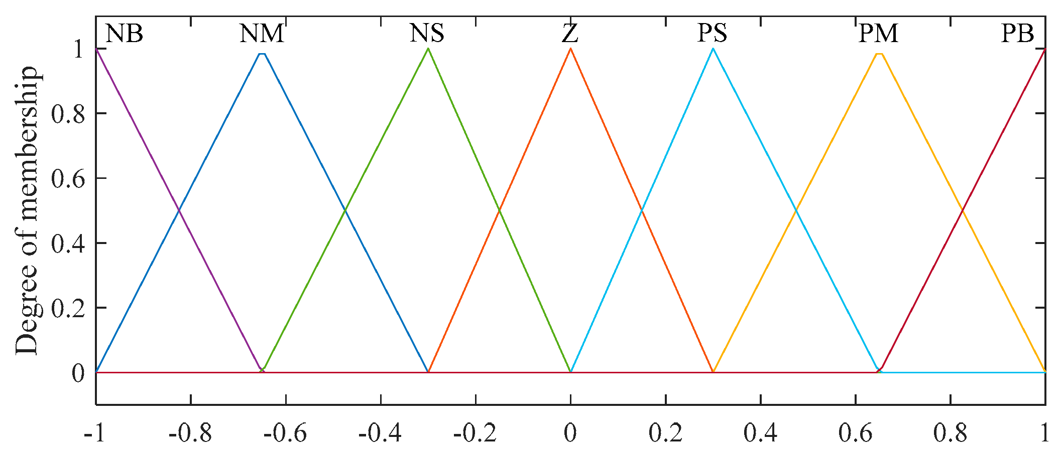
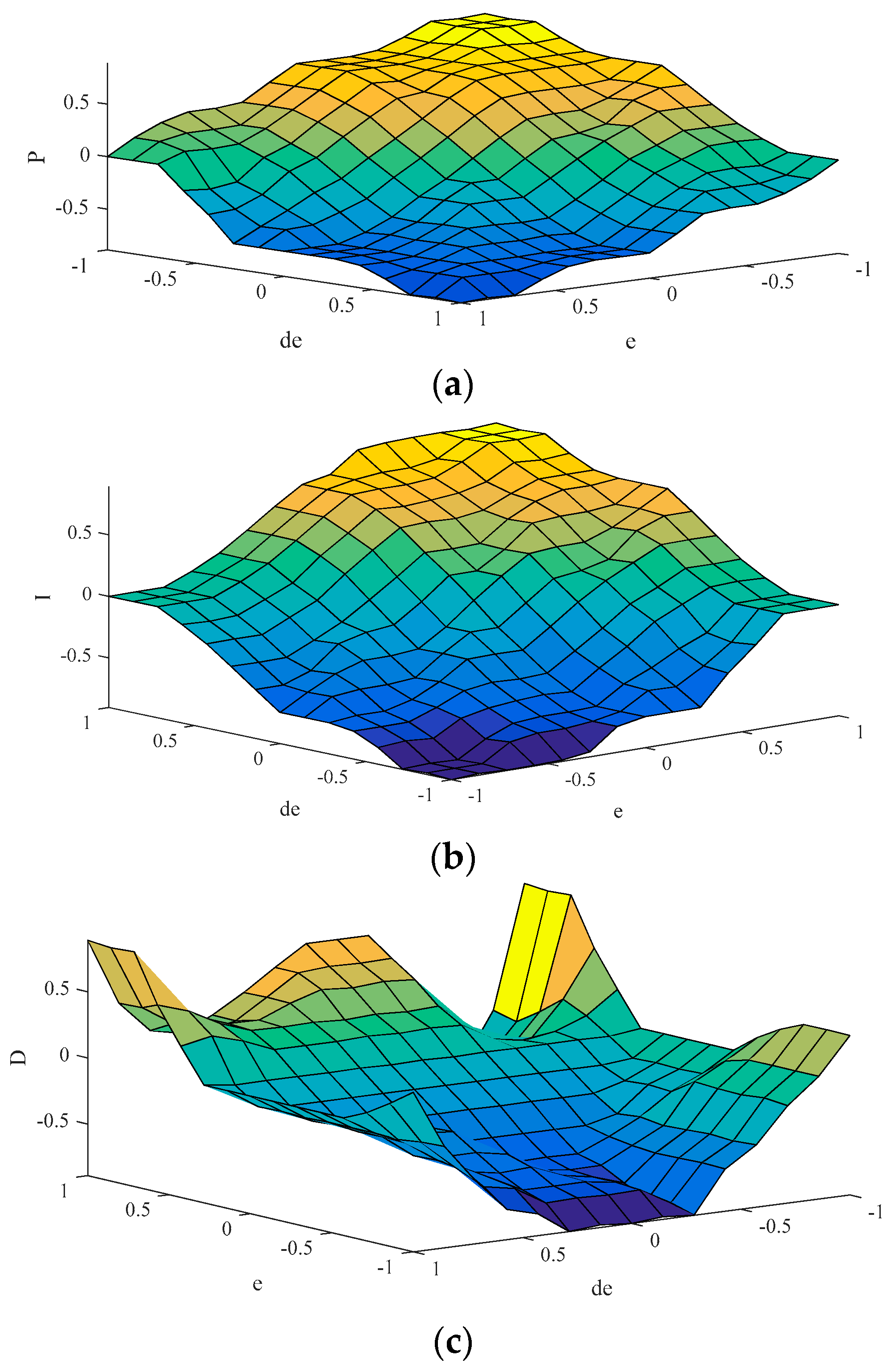
The constants bP, bI, and bD represent a conventional PID controller that provides a good but not optimum system response. These constants can be obtained using any conventional methods for PID controllers. In (2), (3), and (4), the coefficients aP, aI, and aD are obtained according to simulation results to determine the relevant ranges of variations for bP, bI, and bD, respectively. The parameters of P, I, and D onlines are determined by the fuzzy rules in Figure 3. Membership functions for inputs and outputs are shown in Figure 3. The vertical axes represent the degree of membership that is within the range of [0, +1].
The meaning of the linguistic variables is listed in Table 1.
4. PRD Method for WT Based on Fatigue Load Sensitivity Using Quadratic Programming Algorithm
In the wind farm power reference dispatch section, the power reference dispatch controller regulates all the WT active outputs of the wind farm. The controller aims to minimize the fatigue load of WT and track the active power allocated by the frequency adjustment controller. Typically, the sampling time of the wind farm controller is in seconds [28]. Therefore, the rapid dynamics of generators and pitch actuators can be ignored [37]. In addition, shaft torsion and tower point oscillations are ignored to reduce the complexity of the model.
The fatigue loads of WTs can be divided into two parts: one is aerodynamic loads and gravity loads (external), and the other is structural loads (internal) [38]. In this paper, the fatigue loads mainly focus on the loads of the drive train due to the torsion of the shaft and the loads of the tower structure due to the tower deflection. Compared with static loads, the dynamic stress causing structural damage of WTs is a much bigger issue. By reducing the fluctuations of low-speed shaft torque Ts and thrust force Ft, the related fatigue loads can be reduced. can be represented by a combination of and when the drive train and tower structure loads are considered.
4.1. Improved Model of Fatigue Load Sensitivity
The WT (NREL 5 MW) developed by the National Renewable Energy Laboratory (NREL) is used in this paper [39,40]. The oscillations in the shaft torsion and tower nodding are disregarded, the fluctuations of wind speed are ignored based on the previous report [30]. In order to better optimize the calculation, the equations of fatigue load sensitivity are re-derived. In the process of the optimization dispatch, the redefined fatigue load sensitivity will be used. The active power of the WT output is still controlled by adjusting the pitch angle and torque.
The equivalent mass Jt of drive train system is described by [41]
where Jr is the rotor mass; Jg is the generator mass; ηg is the gear box ratio.
The low-shaft motion equation is described by
where ωr is the measured rotor speed; Trot is the aerodynamic torque; Tg is the generator torque;
The measured generator speed ωg is filtered by a low-pass filter and the filtered speed ωf is
where τf is time constant of the filter of ωg.
According to the deviation of ωf from generator rated speed ωg-rated, pitch angle reference θref can be obtained by the PI controller.
where kp is the proportional gain; ki is the integral gain; ka is a function of θref, defined by . Where ka1 and ka2 are the constants.
By defining
(8) is transformed into
According to the motion equation of shaft torque Ts, , and can be described by
where ωg is the measured generator speed; B is the main shaft viscous friction coefficient.
According to (11) and (12), can be expressed by
The time of the operating point is assumed to be k. The wind speed v is a variable that can be estimated or measured [42]. In this study, v is estimated. The value at t = k is v0 and is assumed to be constant over a short control period. The measured power output, generator speed, filtered speed, and pitch angle are defined as Pg0, ωg0, ωf0, and θ0 at t = k, respectively. The Trot and Tg at t = k can be defined as Trot0 and Tg0, respectively.
Based on (6), (7), (10), and (13), the incremental form can be obtained as
The aerodynamic torque Trot is calculated by
where R is the length of the blade; ρ is the air density; v is the wind speed on the rotor; Cp is the power coefficient; λ is the tip speed ratio, defined by ; In order to simplify the expression, Psim is defined by .
According to (18), ΔTrot can be calculated by
where Cp is described in a lookup table derived from the inputs λ and θ, as is shown in Table 2. Where n and m are the corresponding rows and columns, respectively.
The generator torque reference Tg_ref is filtered by a low-pass filter and the generator torque Tg is derived by,
where τg is the time constant of the filter of Tg_ref. Tg_ref is calculated by
According to (23) and (24), ΔTg and ΔTg_ref can be calculated by
where Δt is the control cycle.
According to (14)–(17), the continuous state space model for WT is formulated as
where , and the state space matrices are
These matrices change every other dispatch cycle. Then, the continuous state space model is discretized with the sampling period ts, which is
with
Substituting (6) and (11), the shaft torque Ts can be calculated by
Accordingly,
Based on (19) and (25), (30) can be transformed into
with
Based on (28) and (31)
Hence
In order to simplify the expressions, and are defined by
Therefore, the fatigue load sensitivity of the drive train can be expressed as
According to [43], The tower dynamics is not included in the simplified WT model. According to, it is assumed the tower base overturning moment Mt can be approximately derived by
where H is the tower height. Ft is thrust force.
The thrust force Ft is calculated by
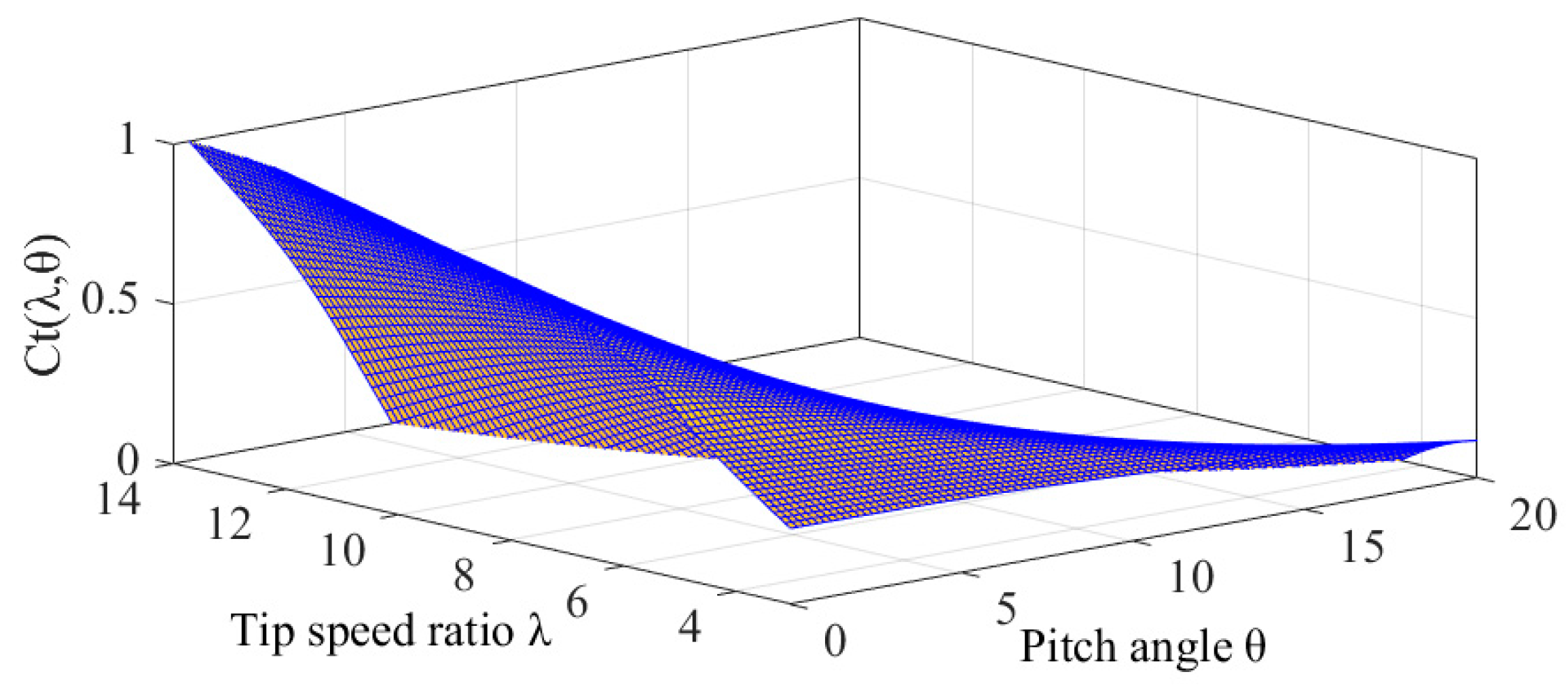
where Ct is the thrust coefficient.
Accordingly
Similar to (31),
with
Based on (28) and (41)
Hence
Similar to (34) and (35),
Therefore, the fatigue load sensitivity of the tower structure can be expressed as
The fatigue load sensitivities considered in the paper are dynamic loads causing structural damage. The equation shown in (33) and (42) are not equations for calculating a fatigue load, but equations for calculating the change in the shaft torque ΔMs and the tower bending moment ΔMt associated with the fatigue load. The parameters in the equation are changing at different times. By reducing ΔMs and ΔMt, the corresponding fatigue load can be reduced. The calculations are carried out by this law of effect. Reductions on the changes of the moments ΔMs and ΔMt are highly corelated to reductions in the damage equivalent fatigue load [44]. ΔMs and ΔMt are related to changes in power reference. ΔMs and ΔMt can be reduced by properly distributing the active power. ΔMs and ΔMt are reduced for each sampling period, so the fatigue loads are reduced.
4.2. Cost Function and Constraints
In Figure 1, every individual WT is equipped with an exclusive control system that can follow the power references provided by the frequency adjustment controller.
The controller minimizes the variation of shaft torque Ts and thrust force Ft to reduce the fatigue load. Accordingly, the cost function is expressed as
For the convenience of calculation, the equivalent calculation formula is expressed as
where ξ is the weight coefficient.
The constraints are expressed by
where is the demanded power of WF; is the maximum available power of WT-i, it can be estimated by
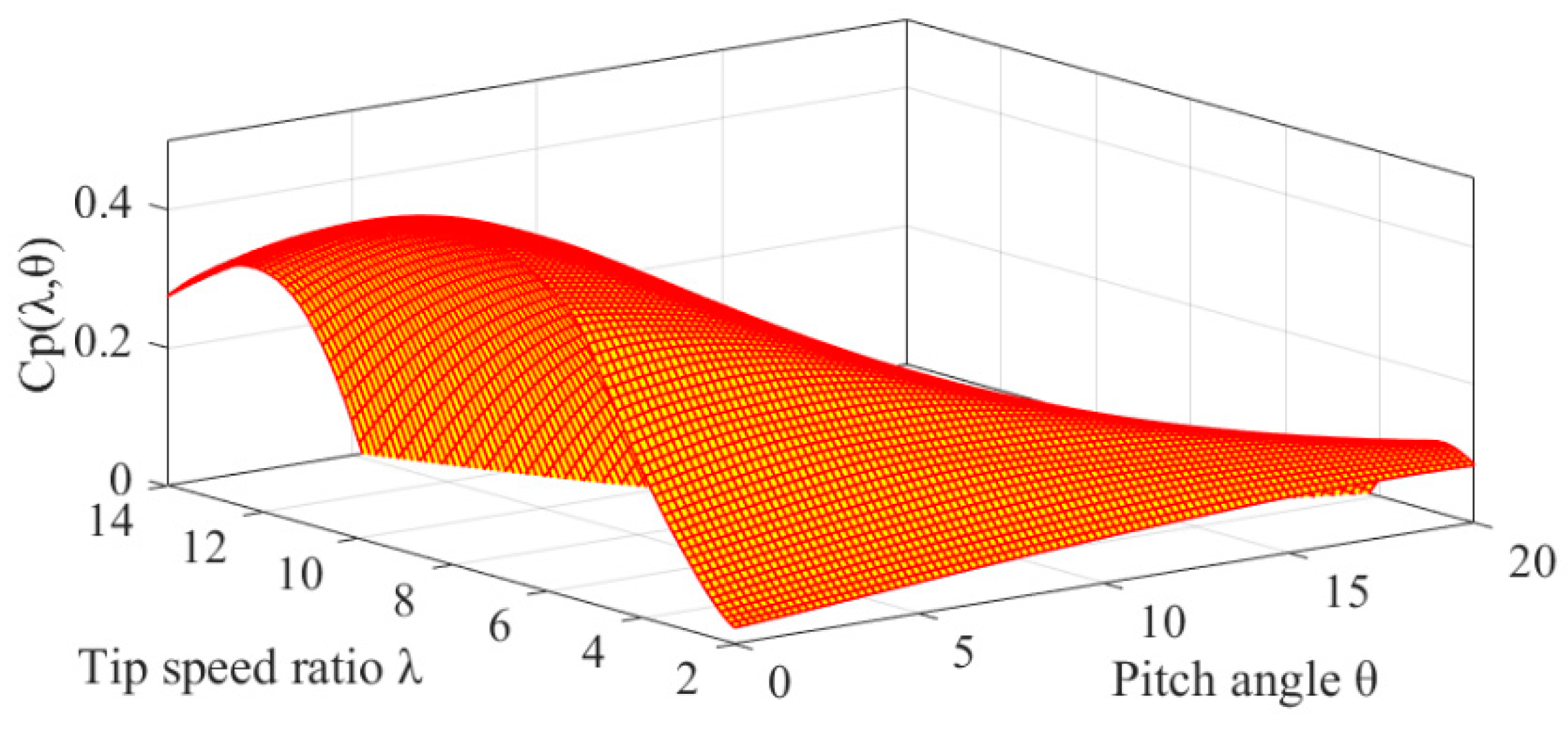
where is the rated power of WT; vnac is the nacelle wind speed of WT. The corresponding data of Cp and Ct for this study can be accessed in the wind turbine model of SimWindFarm. The plot of Cp(λ, θ) and Ct(λ, θ) based on the lookup table is shown in Appendix A.
The presented problems can be expressed as standard quadratic programming (QP) issues [45,46]. It can be effectively solved by a commercial solver. This optimization problem can be solved by different optimization methods. Group intelligent algorithms such as particle swarm optimization (PSO) and genetic algorithm (GA) have good search performance for solving complex problems, but the calculation time is long and is not suitable for real-time online optimization [47,48,49,50]. The programming algorithm has a good ability to search for non-complex solving problems, and the calculation time is short, which is suitable for online optimization. The model proposed in this paper belongs to the non-complex online solution model.
Then, the matrix H and the matrix f of QP can be expressed as
If the available power of WF does not meet the demand, the following procedure is available.
5. Case Study
5.1. System Setup
The WF control architecture illustrated in Figure 1 is used to test the performance of control. Figure 1 shows the typical configuration of a WF, which consists of 10, 5 MW WTs. The simulation model is based on SimWindFarm [40] developed in the EU-FP7 project by AEOLUS. The SimWindFarm model allows the real time simulation of flows in the wind field and includes the main aerodynamic effects of the wind farm in MATLAB/Simulink. It consists of four elementary components: wind turbine dynamics, wind field interactions and dynamics, wind farm controller, and electrical network operator. It can represent the main dynamics of a wind farm. The model toolbox includes a wind field generator where mean wind speed, turbulence intensity, and grid resolution can be specified. Furthermore, a number of post-processing tools are included for performance, such as a rain-flow counting algorithm and wake animation. Simulations are conducted for WF over 200 s of run time.
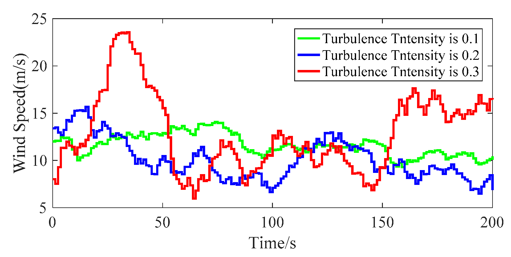
In the test system, the frequency adjustment controller of WF sends instructions every 0.5 s. 0.5 s is to match the wind farm dispatch algorithm and faster to achieve frequency regulation. The parameters of frequency adjustment controller are shown in Table 3. The PRD optimization (OPT) controllers send instructions every 0.5 s. The detailed WT parameters are listed in Table 4. The typical turbulent winds with different intensities generated by the Aeolus toolbox with same average wind speed of 12 m/s are shown in Figure 5.
Through post-processing, the fatigue cycles based on the rainflow counting method are derived to evaluate the performance of the proposed method. Furthermore, the damage equivalent load (DEL) is based on the Miner’s rule and depends on the material properties specified by the slope of the S–N curve for quantizing the load minimization. In this study, the relevant calculations are performed by MCrunch developed by NREL [51].
5.2. Wind Farm Controller Performance
5.2.1. Performance for the Improved Model of Fatigue Load Sensitivity
In the simple WT model, the drive train can be considered to be rigid if the fatigue load is ignored. However, the drive train is a flexible system. A comparison of measured ωr and is shown in Figure 6. As shown in Figure 6, ωr ≠ . So Δωg(k) and Δωr(k) are calculated separately in the improved models, and the calculation formula of is not used.
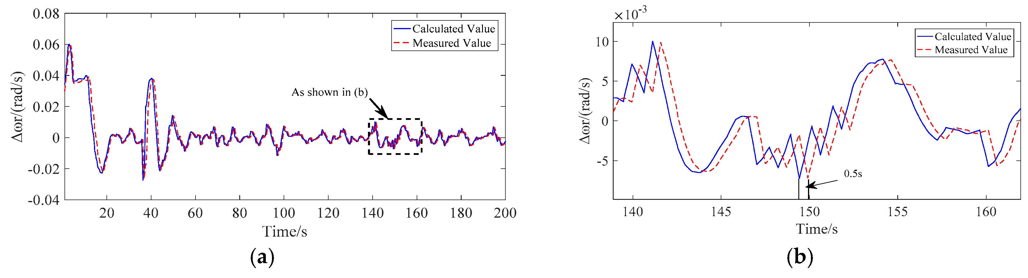
The wind speed of the WF is 12 m/s with 0.1 turbulence intensity. The values of Δωg(k + 1) and Δωr(k + 1) obtained by calculating WT1 are shown in Figure 7 and Figure 8. Note that x(k + 1) is obtained by discretizing x(k). Figure 7, Figure 8, Figure 9 and Figure 10b are enlarged image of the inside of the dashed box in Figure 7, Figure 8, Figure 9 and Figure 10a, which will not be described in detail in the following paper.
As is shown in Figure 7b and Figure 8b, The values of Δωg and Δωr after 0.5 s can be accurately calculated using the improved model. A better basis for optimizing results is provided by this precise calculation.
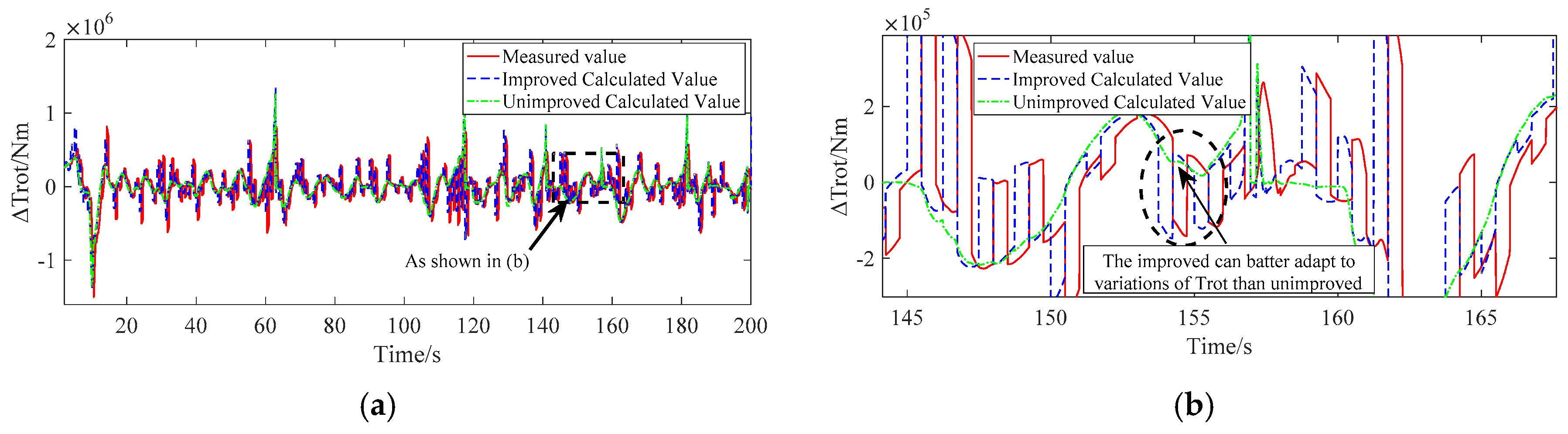
The effect of changes in wind speed is considered when calculating ΔTrot. Comparison of the case of adding and not adding is shown in Figure 9.
The model is simulated based on SimWindFarm. Since the control time is 0.5 s, sampling is performed every 0.5 s. Because Trot is cube of v, even small changes of v can have a big impact on ΔTrot. As is shown in Figure 9b, in the vicinity of 154 s, there is a big step in the measured value, which is caused by the change in wind speed. Mutations in ΔTrot caused by sudden changes in wind speed can still be accurately calculated by the improved model. However, the original models that did not consider cannot adapt to this mutation. The value of ΔTrot after 0.5 s is accurately calculated.
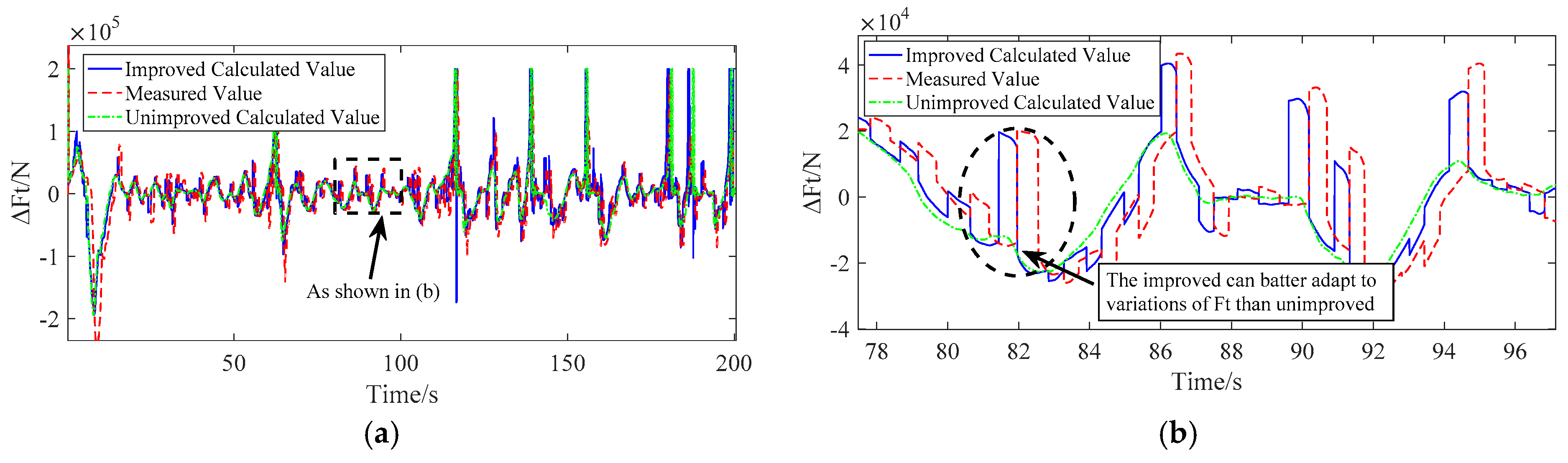
After a detailed improvement, the ΔFt calculation is more accurate. The comparison between the improved value and the measured value is shown in Figure 10.
As is shown in Figure 10b. In the vicinity of 82 s, there is a big step in the measured value, which is caused by the change in wind speed. The improved model can better adapt to the ΔFt mutation like ΔTrot. This improvement makes the calculation of the optimization target more accurate and the optimization effect is better. The re-derived fatigue load sensitivity equations can improve the calculation accuracy very well.
5.2.2. Performance for Different Turbulence Intensity
The normal PRD controller uses a proportional distribution method (NORM). The reference power is assigned to the WT in the available power ratio. As is calculated by
In order to test the efficacy of the improved model, the operation of wind farm under different turbulence intensity were studied and the FAC is not used. The average wind speed of the test wind is 12 m/s, and the turbulence intensity is 0.1, 0.2, and 0.3 respectively. The results of OPT and NORM are compared under different turbulence intensities. The tower bending moment was mainly considered in this paper, so the weight coefficient ξ to 3000 is selected.
Scenario 1: The turbulence intensity is 0.1. The wind farm reference power is 35 MW under this scenario. The calculated DELs of Ts and Mt for all WTs are listed in Table 5. As shown in Table 5, some of the WTs have more growth in DELs for Ts, but this growth will be offset as the simulation time increases. The total DELs of wind farms using OPT is still lower than NORM. From the whole WF point of view, the reductions of the total DEL for Ts is 2.21%.
Compared with the NORM, most DELs of Mt except for NO.2 are reduced. The reduction values are from 0.15% to 16.05%. From the whole WF point of view, the total DEL of Mt is reduced by 5.32%.
Scenario 2: The turbulence intensity is 0.2. The wind farm reference power is 20 MW under this scenario. Scenario 3: The turbulence intensity is 0.3. The wind farm reference power is 15 MW under this scenario. The calculated DELs of Ts and Mt for the sum of all WTs are listed in Table 6.
When the turbulence intensity is 0.2, a more detailed cumulative rainflow cycle is shown in Figure 11. A representative WT (WT09) is used as an example. Compared with the NORM, less cycles are found for OPT, which implies less fatigue loads experienced by the WT.
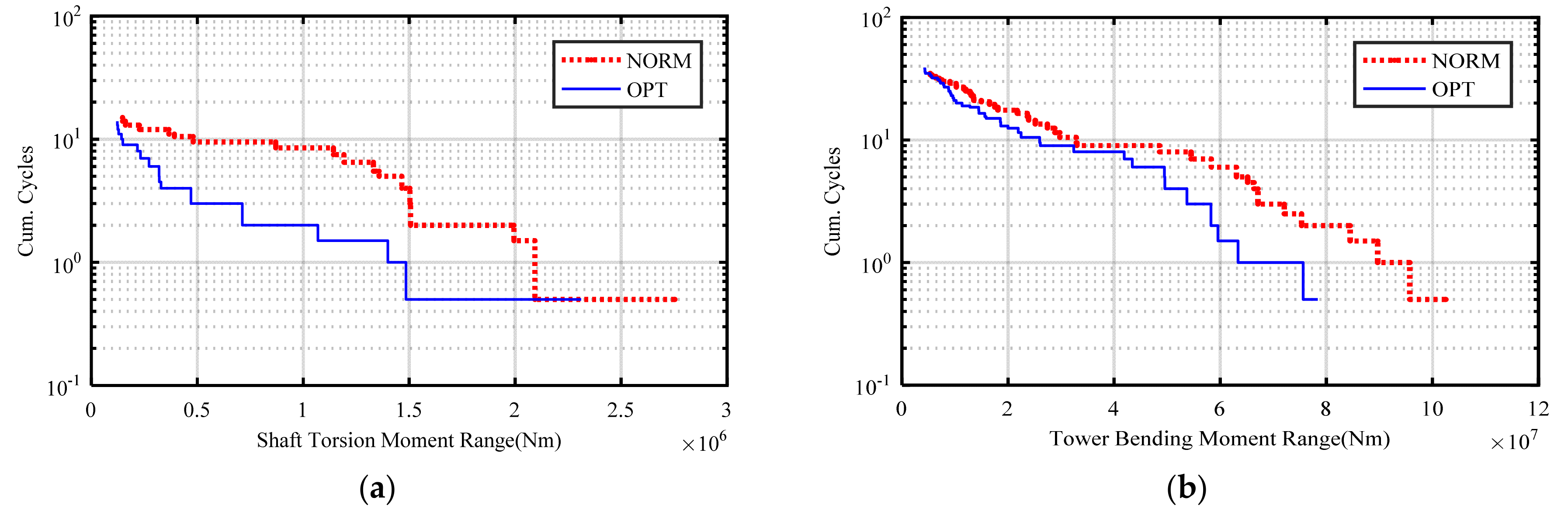
When the turbulence intensity is 0.3, a more detailed cumulative rainflow cycle is shown in Figure 12. A representative WT02 is used as an example. Compared with the NORM, less cycles are found for OPT, which implies less fatigue loads experienced by the WT.
Fatigue load optimization results with three different turbulence intensities were obtained. It can be seen from the results that the improved model can optimize the fatigue load well under different turbulence intensities.
5.3. Overall Performance
5.3.1. WF Controller Performance
In order to prove the performance of the frequency control of the developed solution, the wind farm is assumed to be able to get enough power from the wind. When the WF is operating in the frequency regulation mode, the measured grid frequency is used as a feedback signal to establish real-time active power control. The baseline model for electrical network operator in SimWindFarm can function in different power command modes such as: absolute, delta, and frequency regulation modes. Basically, baseline control scheme in frequency regulation mode can maintain the necessary balance between power generation and loads. The demand power of the baseline control is calculated by
where td and tc are two constants (tc > td) of dead bands and control bands, defined by td = 0.002 and tc = 0.02 which can enable the baseline control to function optimally. Moreover, Pup and Pdown are defined by
where Pmin and Pmax are the prescribed minimum and maximum limits for the total power of WF.
In order to verify the performance of the control method, different functions of the grid load are defined and used for WF testing. Baseline control is compared to Fuzzy-PID. NORM dispatch method is compared to OPT method. The initial frequency is assumed to be 50 Hz. The test wind is 12 m/s with 0.3 turbulence intensity. Figure 13a and Figure 14a show the performance of the active power control method for the WF in response to the different loads considered, respectively. Figure 13b and Figure 14b show the grid frequency responses with respect to the different loads, respectively. The power and frequency responses of Fuzzy-PID and baseline control are compared in Figure 13 and Figure 14, respectively. The power curve of the wind farm output is the same whether the WF dispatch method uses NORM or OPT.
As shown in Figure 13a, the grid load A is a step variable. As is shown in Figure 13b, the baseline control cannot achieve a frequency of 50 Hz, and there is still an error of 0.004 Hz as the control time increases. The frequency error of the Fuzzy-PID control method is smaller than that of the baseline control. As the control time increases, the frequency gradually approaches 50 Hz and the error disappears. The Fuzzy-PID control method can quickly track the frequency so that the error is approximately zero at the 100 s. Therefore, the Fuzzy-PID method has better control effects than the baseline control.
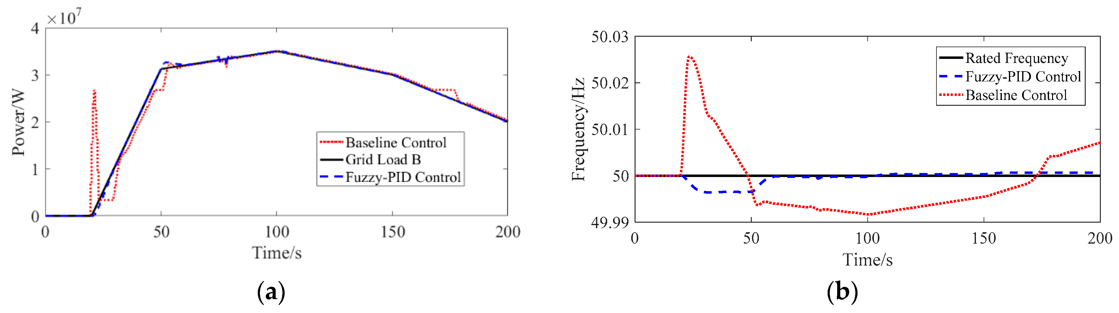
As is shown in Figure 14a, grid load B is the varying load. Baseline control failed to track the grid load during the initial phase of 20–50 s, which also caused a relatively large frequency fluctuation of 20–50 s as shown in Figure 14b. Fuzzy-PID control can track grid load very well by compared to baseline control. As is shown in Figure 14b, Fuzzy-PID can track the frequency very well, and the frequency error of Fuzzy-PID is smaller. As are shown in Figure 13 and Figure 14, less power fluctuations make power tracking better.
To check the tracking accuracy of APC methods, the normalized root-mean-squared error (NRMSE) is defined as
To illustrate the ability of Fuzzy-PID methods in the regulation of the grid frequency, Table 7 quantitatively compares the obtained grid frequency responses in terms of standard deviation (SD) and NRMSE of power responses.
For a step grid load like A, compared to baseline control, NRMSE for power responses increased by 22.02%, and SD for grid frequency responses is reduced by 88.45%. For a varying grid load like B, compared to baseline control, NRMSE for power responses is reduced by 73.15% and SD for grid frequency responses is reduced by 81.88%.
By testing the control method of the WF with different loads, the Fuzzy-PID control has a good performance regardless of the speed or error of the tracking frequency.
5.3.2. Fatigue Loads Performance
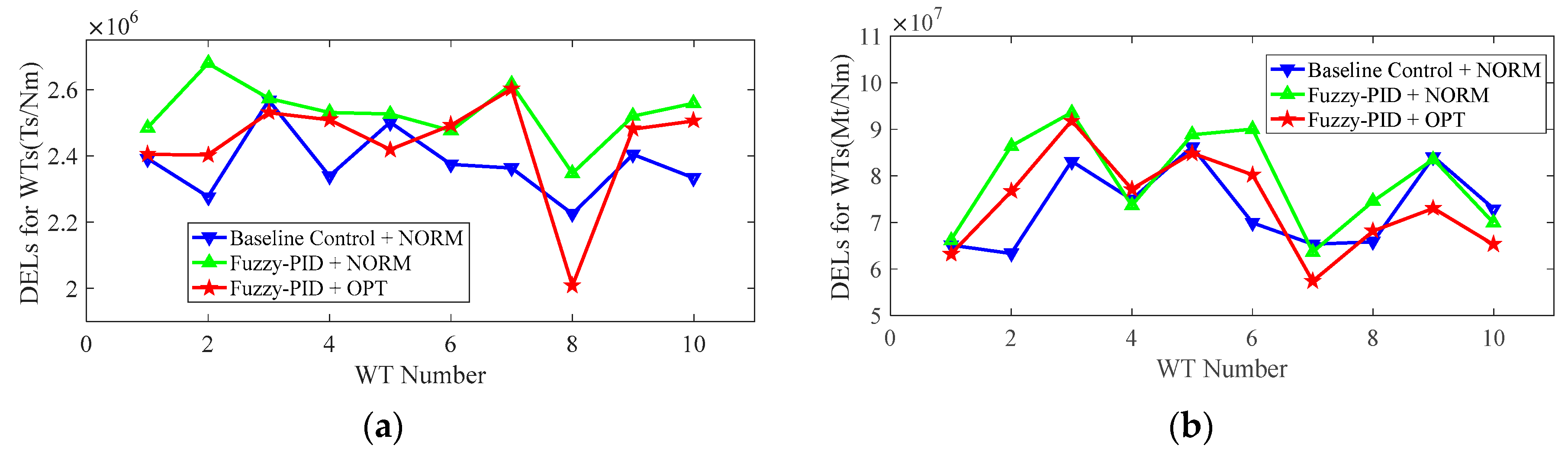
The fatigue load results of the WTs using Baseline Control + NORM, Fuzzy-PID + NORM and Fuzzy-PID + OPT are shown in Figure 15 when load B is used to test the overall controller.
As is shown in Figure 15, the frequency adjustment effect by the Fuzzy-PID is better, but the DELs of Ts is significantly larger than Baseline Control + NORM. The specific results are shown in Table 7, the fatigue load using Fuzzy-PID + NORM increased by 6.47% compared with the fatigue load using Baseline Control + NORM. The fatigue load using Fuzzy-PID + OPT still increased by 2.44% compared with Baseline Control + NORM, but decreased by 3.79% compared with Fuzzy-PID + NORM.
The fatigue load of Mt using Fuzzy-PID + NORM was significantly higher than that of Baseline Control + NORM, and the specific results were increased by 8.15% as shown in Table 8. The fatigue load using Fuzzy-PID + OPT is 0.32% higher than Baseline Control + NORM and 7.24% lower than Fuzzy-PID + NORM.
The fatigue load of the WT will increase since the WF needs to frequently change the pitch angle and reference power when participating in frequency regulation. The better the frequency adjustment effect, the more frequent this change, the greater the fatigue load caused. The overall fatigue load of the WT is reduced, DELs of Mt is hardly affected especially after considering the fatigue load.
6. Conclusions
In this paper, an APC method for supporting grid frequency regulation in WFs considering fatigue load of WT is proposed. The Fuzzy-FID control is used for a frequency adjustment controller to maintain the balance between power generation and grid load. The equations of fatigue load sensitivity are re-derived. The calculation accuracy is improved by the re-derived equations. The re-derived equations are used for PRD to minimize the fatigue load for all the WTs. Case studies show that the frequency adjustment control method based on Fuzzy-PID can respond to and recover grid frequency deviations more quickly. Less power fluctuations make power tracking better. Compared to baseline control, NRMSE for power responses and SD for grid frequency of Fuzzy-PID are reduced by 81.45% and 81.88%, separately. In addition, the explicit analytical equations of fatigue load sensitivity are re-derived to improve the calculation accuracy of the fatigue loads. DELs for Ts reduced by 2.21% to 5.13%, DELs for Mt reduced by 5.32% to 7.32%. This improvement minimizes fatigue loads for wind farms under different turbulent wind and different loads. The proposed solution is suitable for real-time control of large-scale WF.
Since this study is mainly focused on the wind farm control level, some of the dynamics of WTs are ignored. Rainflow counting is applied to the time histories of thrust and torque from the simulation results, so the evaluation of fatigue load cannot be fully reflected. Quantitative conclusions are uncertain and can only represent trends in fatigue load changes. Since this study is a simulation based on SimWindFarm, the study cannot consider all practical engineering problems. Verifying this method in engineering is what we will do next.
Author Contributions
The paper was a collaborative effort among the authors. Y.W. carried out relevant theoretical research, performed the simulation, analyzed the data, and wrote the paper. Y.L. and X.W. provided critical comments. J.Z. and W.H.L. revised the paper.
Funding
This work was supported by the National Natural Science Foundation (51677121) of China and Liaoning Provincial Department of Education Serves Local Project (201734134).
Conflicts of Interest
The authors declare no conflict of interest.
Nomenclature
| Symbols | |
| KP, KI, KD | Calculated by Fuzzy-PID controller |
| bP, bI, bD | Parameters of conventional PID controller |
| aP, aI, aD | Parameters of determined the relevant ranges of variations for bP, bI, and bD |
| P, I, D | Calculated by Fuzzy Rules |
| Demanded power of wind farm | |
| Available power of wind farm | |
| Available power of wind turbine i | |
| Rated power of wind farm | |
| Reference power of wind turbine i | |
| Sensitivity of fatigue load with respect to demanded power of wind turbine | |
| Sensitivity of drive train fatigue load with respect to demanded power of wind turbine | |
| Sensitivity of the tower structural fatigue load with respect to demanded power of wind turbine | |
| Grid frequency error | |
| Grid measured frequency | |
| Normal frequency of the grid | |
| Jt | Equivalent mass of the drive-train |
| Jr | Rotational inertia of the rotor |
| Jg | Rotational inertia of the generator |
| ηg | Gear box ratio |
| ωr | Measured rotor speed |
| ωg | Measured generator speed |
| ωg-rated | Rated generator speed |
| Ft | Thrust force |
| Trot | Aerodynamic torque |
| Tg | Generator torque |
| Tg_ref | Generator torque reference |
| Ts | Shaft torque |
| Mt | Tower basefore-aft bending moment |
| Tgiref | Generator torque of wind turbine i |
| ωf | Generator filtered speed |
| τf | Time constant of the filter of ωg |
| τg | Time constant of the filter of Tg_ref |
| θiref | Pitch angle reference of wind turbine i |
| θref | Pitch angle reference of blades |
| ka, β | Functions of θref |
| kp, ki | Proportional and integral gain of θref |
| ka1, ka2 | Constants of ka |
| B | Main shaft viscous friction coefficient |
| Pg0 | Output power of a turbine at t = k |
| ωg0 | Generator speed at t = k |
| ωf0 | Filtered speed of the generator speed at t = k |
| θ0 | Pitch angle at t = k |
| Trot0 | Aerodynamic torque at t = k |
| Tg | Generator torque at t = k |
| R | Length of the blade |
| H | Tower height |
| ρ | Air density |
| v | Wind speed of hub height |
| Cp | Power coefficient |
| Ct | Thrust coefficient |
| λ | Tip speed ratio |
Appendix A
Figure A1.
Cp(λ, θ) based on the data from SimWindFarm.

Figure A2.
Ct(λ, θ) based on the data from SimWindFarm.
References
- Sun, X.J.; Huang, D.G. An Explosive Growth of Wind Power in China. Int. J. Green. Energy 2014, 14, 849–860. [Google Scholar] [CrossRef]
- Nguyen, C.-K.; Nguyen, T.-T.; Yoo, H.-J.; Kim, H.-M. Consensus-Based SOC Balancing of Battery Energy Storage Systems in Wind Farm. Energies 2018, 11, 3507. [Google Scholar] [CrossRef]
- Bottiglione, F.; Mantriota, G.; Valle, M. Power-Split Hydrostatic Transmissions for Wind Energy Systems. Energies 2018, 11, 3369. [Google Scholar] [CrossRef]
- Kazda, J.; Cutululis, N.A. Fast Control-Oriented Dynamic Linear Model of Wind Farm Flow and Operation. Energies 2018, 11, 3346. [Google Scholar] [CrossRef]
- Wind Power Capacity Reaches 539 GW, 52,6 GW Added in 2017. 12 February 2018. Available online: http://wwindea.org/blog/2018/02/12/2017-statistics/ (accessed on 20 April 2019).
- Sun, B.; Tang, Y.; Ye, L.; Chen, C.; Zhang, C.; Zhong, W. A Frequency Control Method Considering Large Scale Wind Power Cluster Integration Based on Distributed Model Predictive Control. Energies 2018, 11, 1600. [Google Scholar] [CrossRef]
- Hou, T.T.; Lou, S.H.; Wu, Y.W. Capacity Optimization of Thermal Units Transmitted with Wind Power: A Case Study of Jiuquan Wind Power Base, China. J. Wind. Eng. Ind. Aerod. 2014, 129, 64–68. [Google Scholar] [CrossRef]
- Dai, X.M.; Zhang, K.F.; Geng, J. Study on Variability Smoothing Benefits of Wind Farm Cluster. Turk. J. Electr. Eng. Comput. Sci. 2018, 26, 1894–1908. [Google Scholar] [CrossRef]
- Du, W.J.; Bi, J.T.; Wang, T.; Hua, W. Impact of Grid Connection of Large-Scale Wind Farms on Power System Small-Signal Angular Stability. CSEE JPES 2015, 1, 83–89. [Google Scholar] [CrossRef]
- Li, J.; Ye, L.; Zeng, Y.; Wang, H.F. A Scenario-Based Robust Transmission Network Expansion Planning Method for Consideration of Wind Power Uncertainties. CSEE JPES 2016, 2, 11–18. [Google Scholar] [CrossRef]
- Liao, S.Y.; Xu, J.; Sun, Y.Z.; Bao, Y.; Tang, B.W. Wide-Area Measurement System-Based Online Calculation Method of PV Systems De-loaded Margin for Frequency Regulation in Isolated Power Systems. IET Renew. Power. Gen. 2018, 12, 335–341. [Google Scholar] [CrossRef]
- Athari, M.H.; Wang, Z. Impacts of Wind Power Uncertainty on Grid Vulnerability to Cascading Overload Failures. IEEE Trans. Sustain. Energy 2018, 9, 128–137. [Google Scholar] [CrossRef]
- You, R.; Barahona, B.; Chai, J.Y.; Cutululis, N.A.; Wu, X.Z. Improvement of Grid Frequency Dynamic Characteristic with Novel Wind Turbine Based on Electromagnetic Coupler. Renew. Energy 2017, 113, 813–821. [Google Scholar] [CrossRef]
- Oest, J.; Lund, E. Topology Optimization with Finite-life Fatigue Constraints. Struct. Multidiscip. Optim. 2017, 56, 1045–1059. [Google Scholar] [CrossRef]
- Attya, A.B.; Domínguez-García, J.L.; Bianchi, F.D.; Anaya-Lara, O. Enhancing Frequency Stability by Integrating Non-conventional Power Sources Through Multi-terminal HVDC Grid. Int. J. Electr. Power Energy Syst. 2018, 95, 128–136. [Google Scholar] [CrossRef]
- Dijk, M.T.V.; Wingerden, J.W.V.; Ashuri, T.; Li, Y. Wind Farm Multi-Objective Wake Redirection for Optimizing Power Production and Loads. Energy 2017, 121, 561–569. [Google Scholar] [CrossRef]
- Soleimanzadeh, M.; Wisniewski, R. Controller Design for a Wind Farm, Considering Both Power and Load Aspects. Mechatronics 2011, 21, 720–727. [Google Scholar] [CrossRef]
- Njiri, J.G.; Beganovic, N.; Do, M.H.; Soffker, D. Consideration of Lifetime and Fatigue Load in Wind Turbine Control. Renew. Energy 2018, 131, 818–828. [Google Scholar] [CrossRef]
- Kanev, S.K.; Savenije, F.J.; Engels, W.P. Active Wake Control: An Approach to Optimize the Lifetime Operation of Wind Farms. Wind Energy 2018, 21, 488–501. [Google Scholar] [CrossRef]
- Madani, S.M.; Akbari, M. Analytical Evaluation of Control Strategies for Participation of Doubly Fed Induction Generator-Based Wind Farms in Power System Short-Term Frequency Regulation. IET Renew. Power Gen. 2014, 8, 324–333. [Google Scholar]
- Leon, A.E.; Mauricio, J.M.; Gomezexposito, A.; Solsona, J.A. Hierarchical Wide-Area Control of Power Systems Including Wind Farms and Facts for Short-Term Frequency Regulation. IEEE Trans. Power Syst. 2012, 27, 2084–2092. [Google Scholar] [CrossRef]
- Ye, H.; Pei, W.; Qi, Z. Analytical Modeling of Inertial and Droop Responses from a Wind Farm for Short-Term Frequency Regulation in Power Systems. IEEE Trans. Power Syst. 2015, 31, 3414–3423. [Google Scholar] [CrossRef]
- Wang, Z.; Wu, W. Coordinated Control Method for DFIG-Based Wind Farm to Provide Primary Frequency Regulation Service. IEEE Trans. Power Syst. 2017, 33, 3644–3659. [Google Scholar] [CrossRef]
- Gao, Y.; Ai, Q. Distributed Multi-agent Control for Combined AC/DC Grids With Wind Power Plant Clusters. IET Gener. Transm. Dis. 2018, 12, 670–677. [Google Scholar] [CrossRef]
- Gao, X.D.; Meng, K.; Dong, Z.Y. Cooperation-Driven Distributed Control Method for Large-Scale Wind Farm Active Power Regulation. IEEE Trans. Energy Convers. 2017, 32, 1240–1250. [Google Scholar] [CrossRef]
- Badihi, H.; Zhang, Y.; Hong, H. Active Power Control Design for Supporting Grid Frequency Regulation in Wind Farms. Annu. Rev. Control. 2015, 40, 70–81. [Google Scholar] [CrossRef]
- Knudsen, T.; Bak, T.; Svenstrup, M. Survey of Wind Farm Control-Power and Fatigue Optimization. Wind Energy 2015, 18, 1333–1351. [Google Scholar] [CrossRef]
- Zhao, H.R.; Wu, Q.W.; Guo, Q.; Sun, H.B.; Xue, Y.S. Distributed Model Predictive Control of a Wind Farm for Optimal Active Power Control—Part II: Implementation with Clustering-Based Piece-Wise Affine Wind Turbine Model. IEEE Trans. Sustain. Energy 2015, 6, 840–849. [Google Scholar] [CrossRef]
- Zhao, H.R.; Wu, Q.W.; Guo, Q.; Sun, H.B.; Xue, Y.S. Optimal Active Power Control of a Wind Farm Equipped with Energy Storage System Based on Distributed Model Predictive Control. IET Gener. Transm. Distrib. 2016, 10, 669–677. [Google Scholar] [CrossRef]
- Zhao, H.R.; Wu, Q.W.; Huang, S.J.; Shahidehpour, M.; Guo, Q.; Sun, H.B. Fatigue Load Sensitivity Based Optimal Active Power Dispatch for Wind Farms. IEEE Trans. Sustain. Energy 2017, 8, 1247–1259. [Google Scholar] [CrossRef]
- Yuan, S.; Zhao, C.; Guo, L. Uncoupled PID Control of Coupled Multi-Agent Nonlinear Uncertain Systems. J. Syst. Sci. Complex. 2018, 31, 4–21. [Google Scholar] [CrossRef]
- Zhang, M.; Rosales, L.P.B.; Ortega, R.; Liu, Z.; Su, H. Pid, Passivity-Based Control of Port-Hamiltonian Systems. IEEE Trans. Autom. Control 2018, 63, 1032–1044. [Google Scholar] [CrossRef]
- Mahto, T.; Mukherjee, V. Fractional Order Fuzzy PID Controller for Wind Energy-Based Hybrid Power System Using Quasi-Oppositional Harmony Search Algorithm. IET Gener. Transm. Dis. 2017, 11, 3299–3309. [Google Scholar] [CrossRef]
- Gil, P.; Sebastião, A.; Lucena, C. Constrained Nonlinear-Based Optimisation Applied to Fuzzy PID Controllers Tuning. Asian J. Control 2018, 20, 135–148. [Google Scholar] [CrossRef]
- Amirhossein, A.; Reza, S.; Ali, J. Performance and Robustness of Optimal Fractional Fuzzy PID Controllers for Pitch Control of a Wind Turbine Using Chaotic Optimization Algorithms. ISA Trans. 2018, 79, 27–44. [Google Scholar]
- Mohan, V.; Chhabra, H.; Rani, A.; Singh, V. An Expert 2DOF Fractional Order Fuzzy PID Controller for Nonlinear Systems. Neural Comput. Appl. 2018, 1–18. [Google Scholar] [CrossRef]
- Vedrana, S.; Mate, J.; Baotić, M. Wind Turbine Power References in Coordinated Control of Wind Farms. Autom. J. Control Meas. Electron. Comput. Commun. 2011, 52, 82–94. [Google Scholar]
- Barlas, T.K.; Kuik, G.A.M.V. Review of State of the Art in Smart Rotor Control Research for Wind Turbines. Prog. Aerosp. Sci. 2010, 46, 1–27. [Google Scholar] [CrossRef]
- Jonkman, J.M.; Butterfield, S.; Musial, W.; Scott, G. Definition of a 5-MW Reference Wind Turbine for Offshore System Development; National Renewable Energy Lab.: Lakewood, CO, USA, 2009. [Google Scholar]
- Grunnet, J.D.; Soltani, M.; Knudsen, T.; Kragelund, M.N.; Bak, T. Aeolus Toolbox for Dynamic Wind Farm Model, Simulation and Control. In Proceedings of the European Wind Energy Conference & Exhibition, Warsaw, Poland, 20–23 April 2010. [Google Scholar]
- Pardalos, P.M.; Rebennack, S.; Pereira, M.V.F.; Iliadis, N.A.; Pappu, V. Handbook of Wind Power Systems; Springer: Berlin, Germany, 2014. [Google Scholar]
- Soltani, M.N.; Knudsen, T.; Svenstrup, M.; Wisniewski, R.; Brath, P.; Ortega, R.; Johnson, K. Estimation of Rotor Effective Wind Speed: A Comparison. IEEE Trans. Control Syst. Technol. 2013, 21, 1155–1167. [Google Scholar] [CrossRef]
- Manwell, J.F.; Mcgowan, J.G.; Rogers, A.L. Wind Energy Explained: Theory, Design and Application, 2nd ed.; John Wiley & Sons: Hoboken, NJ, USA, 2002. [Google Scholar]
- Simley, E.; Dunne, F.; Laks, J.; Pao, L.Y. 10 Lidars and Wind Turbine Control—Part 2. DTU Wind Energy-E-Report-0029. Available online: http://citeseerx.ist.psu.edu/viewdoc/download;jsessionid=16F5DC8769E46EEC0A5834631C48C1E0?doi=10.1.1.361.2830&rep=rep1&type=pdf (accessed on 21 April 2019).
- Luis, V.; Salvador, J. Quadratic programming. J. Oper. Res. Soc. 2013, 16, 256–257. [Google Scholar]
- Cimini, G.; Bemporad, A. Exact Complexity Certification of Active-Set Methods for Quadratic Programming. IEEE Trans. Autom. Control. 2017, 62, 6094–6109. [Google Scholar] [CrossRef]
- Bao, Y.; Xiong, T.; Hu, Z. PSO-MISMO Modeling Strategy for Multistep-Ahead Time Series Prediction. IEEE Trans. Cybern. 2014, 44, 655–668. [Google Scholar] [PubMed]
- Nery, G.A., Jr.; Martins Márcio, A.F.; Kalid, R. A PSO-Based Optimal Tuning Strategy for Constrained Multivariable Predictive Controllers with Model Uncertainty. ISA Trans. 2014, 53, 560–567. [Google Scholar] [CrossRef]
- Sahu, R.K.; Panda, S.; Chandra Sekhar, G.T. A Novel Hybrid PSO-PS Optimized Fuzzy PI Controller for AGC in Multi Area Interconnected Power Systems. Int. J. Elec. Power 2015, 64, 880–893. [Google Scholar] [CrossRef]
- Gong, D.W.; Sun, J.; Miao, Z. A Set-Based Genetic Algorithm for Interval Many-Objective Optimization Problems. IEEE Trans. Evol. Comput. 2016, 22, 47–60. [Google Scholar] [CrossRef]
- Buhl, M. MCrunch User’s Guide for Version 1.00, 1st ed.; National Renewable Energy Laboratory: Lakewood, CO, USA, 2008. [Google Scholar]
Figure 1.
Architecture of active power control for WF.
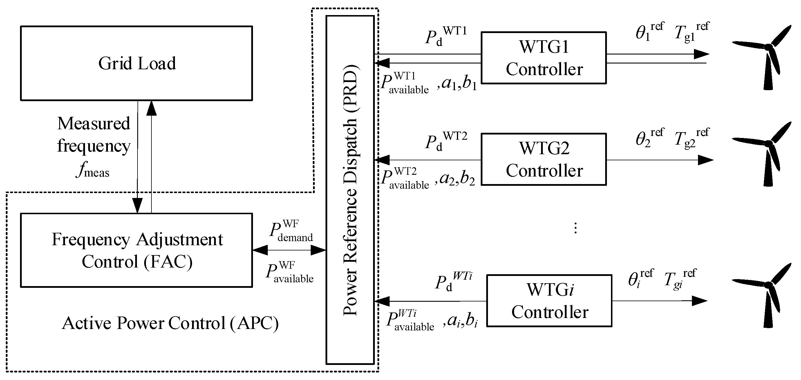
Figure 2.
Fuzzy-PID controller.
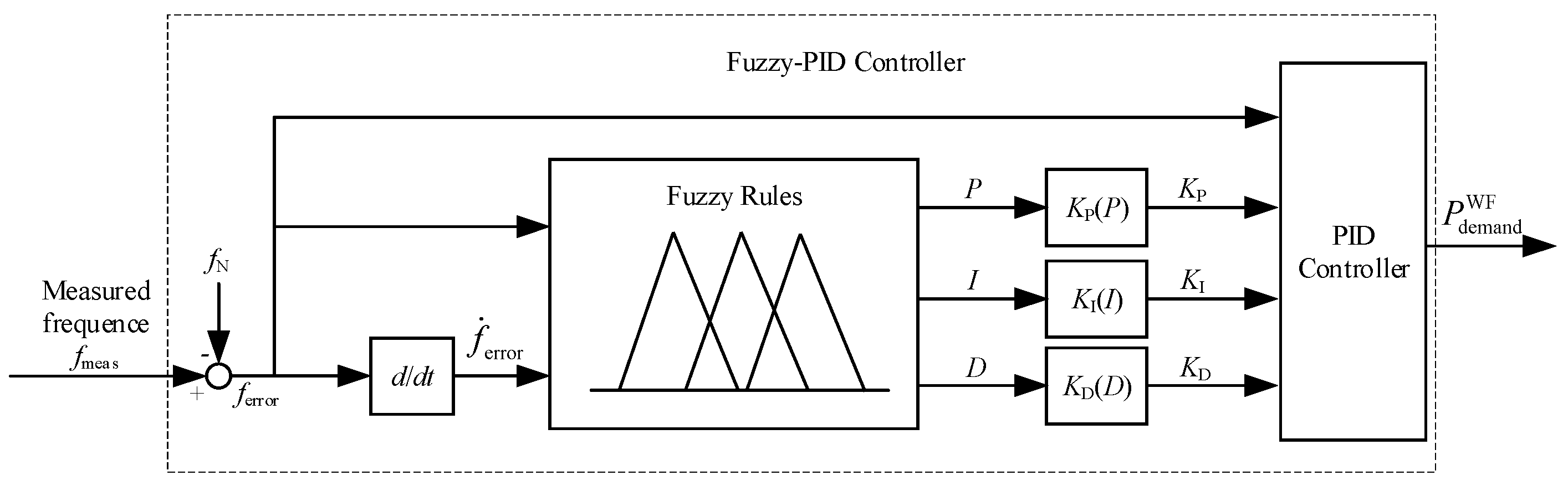
Figure 3.
Membership functions for inputs and outputs.

Figure 4.
Control signal of P, I and D after defuzzification. (a) Control signal of P after defuzzification.; (b) Control signal of I after defuzzification.; (c) Control signal of D after defuzzification.
Figure 4.
Control signal of P, I and D after defuzzification. (a) Control signal of P after defuzzification.; (b) Control signal of I after defuzzification.; (c) Control signal of D after defuzzification.

Figure 5.
Typical turbulent winds with different intensities generated by the Aeolus toolbox with same average wind speed of 12 m/s.
Figure 5.
Typical turbulent winds with different intensities generated by the Aeolus toolbox with same average wind speed of 12 m/s.

Figure 6.
Wind speed, and the measured ωr and in a flexible system.
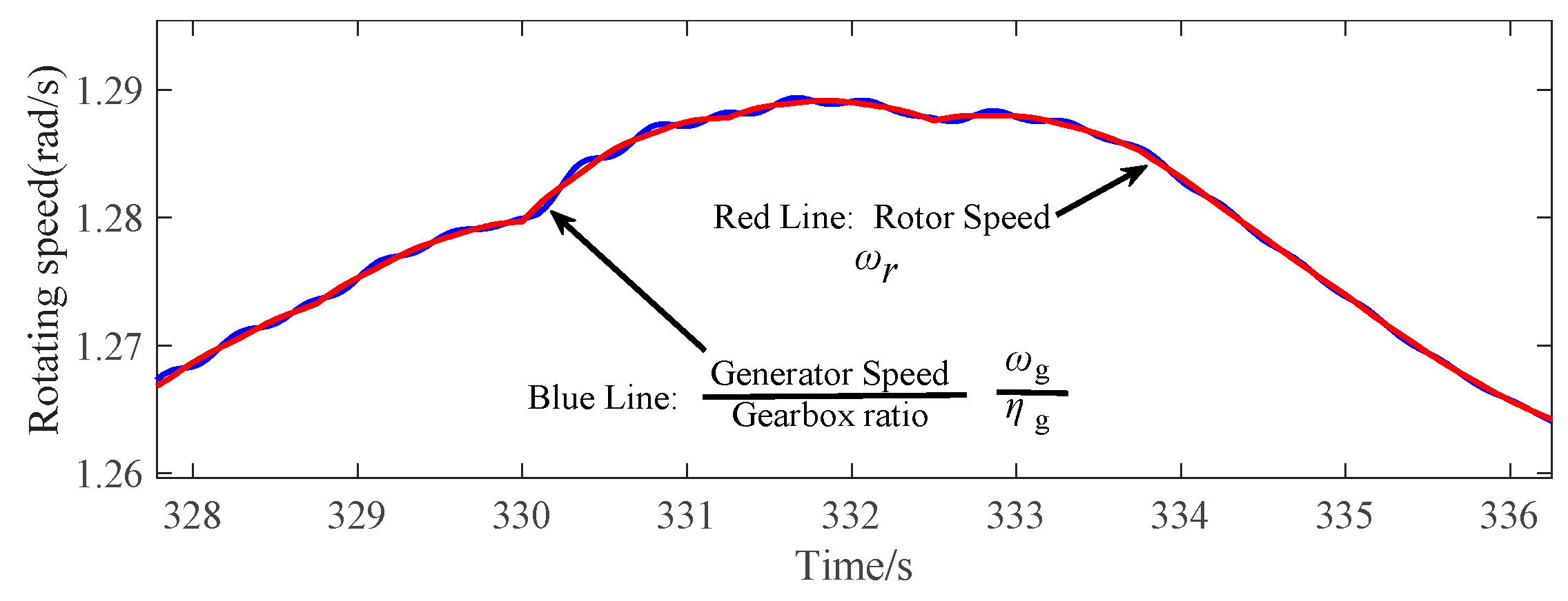
Figure 7.
Calculated and measured values of Δωg. (a) Calculated and measured values of Δωg from 0 to 200 seconds; (b) Calculated and measured values of Δωg from 89 to 106 seconds.
Figure 7.
Calculated and measured values of Δωg. (a) Calculated and measured values of Δωg from 0 to 200 seconds; (b) Calculated and measured values of Δωg from 89 to 106 seconds.
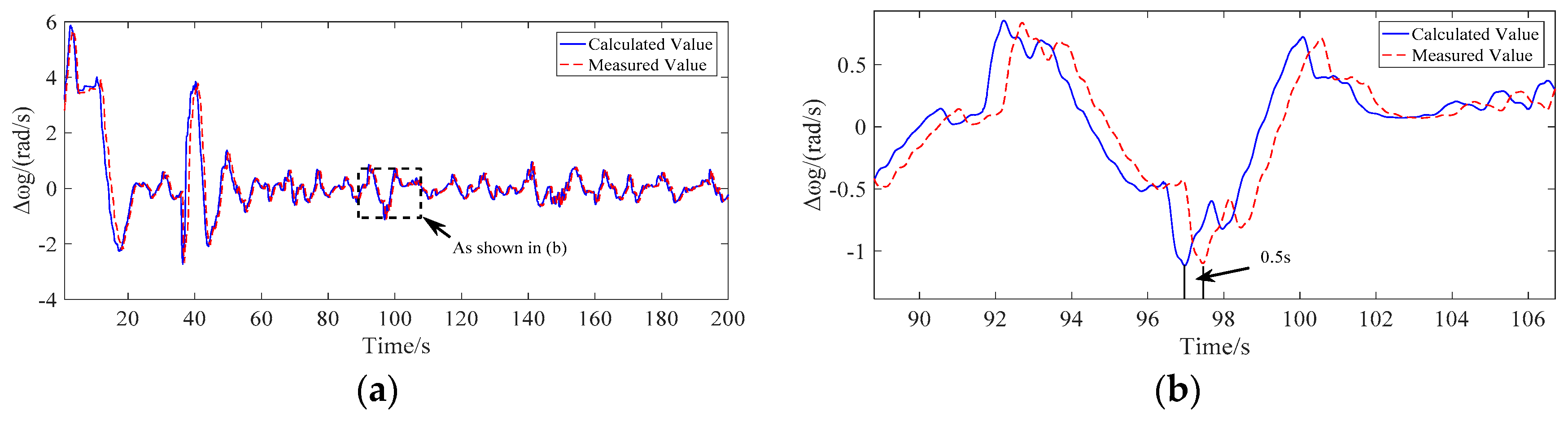
Figure 8.
Calculated and measured values of Δωr. (a) Calculated and measured values of Δωr from 0 to 200 seconds; (b) Calculated and measured values of Δωr from 139 to 162 seconds.
Figure 8.
Calculated and measured values of Δωr. (a) Calculated and measured values of Δωr from 0 to 200 seconds; (b) Calculated and measured values of Δωr from 139 to 162 seconds.

Figure 9.
Calculated and measured values of ΔTrot. (a) Calculated and measured values of ΔTrot from 0 to 200 seconds; (b) Calculated and measured values of ΔTrot from 144 to 167 seconds.
Figure 9.
Calculated and measured values of ΔTrot. (a) Calculated and measured values of ΔTrot from 0 to 200 seconds; (b) Calculated and measured values of ΔTrot from 144 to 167 seconds.

Figure 10.
Calculated and measured values of ΔFt. (a) Calculated and measured values of ΔFt from 0 to 200 seconds; (b) Calculated and measured values of ΔFt from 78 to 97 seconds.
Figure 10.
Calculated and measured values of ΔFt. (a) Calculated and measured values of ΔFt from 0 to 200 seconds; (b) Calculated and measured values of ΔFt from 78 to 97 seconds.

Figure 11.
Cumulative rainflow cycle of Ts and Mt of WT09 for 0.2 turbulence intensity. (a) Cumulative rainflow cycle of Shaft Torsion Moment for 0.2 turbulence intensity; (b) Cumulative rainflow cycle of Tower Bending Moment for 0.2 turbulence intensity.
Figure 11.
Cumulative rainflow cycle of Ts and Mt of WT09 for 0.2 turbulence intensity. (a) Cumulative rainflow cycle of Shaft Torsion Moment for 0.2 turbulence intensity; (b) Cumulative rainflow cycle of Tower Bending Moment for 0.2 turbulence intensity.

Figure 12.
Cumulative rainflow cycle of Ts and Mt of WT02 for 0.3 turbulence intensity. (a) Cumulative rainflow cycle of Shaft Torsion Moment of WT02 for 0.3 turbulence intensity; (b) Cumulative rainflow cycle of Tower Bending Moment of WT02 for 0.3 turbulence intensity.
Figure 12.
Cumulative rainflow cycle of Ts and Mt of WT02 for 0.3 turbulence intensity. (a) Cumulative rainflow cycle of Shaft Torsion Moment of WT02 for 0.3 turbulence intensity; (b) Cumulative rainflow cycle of Tower Bending Moment of WT02 for 0.3 turbulence intensity.
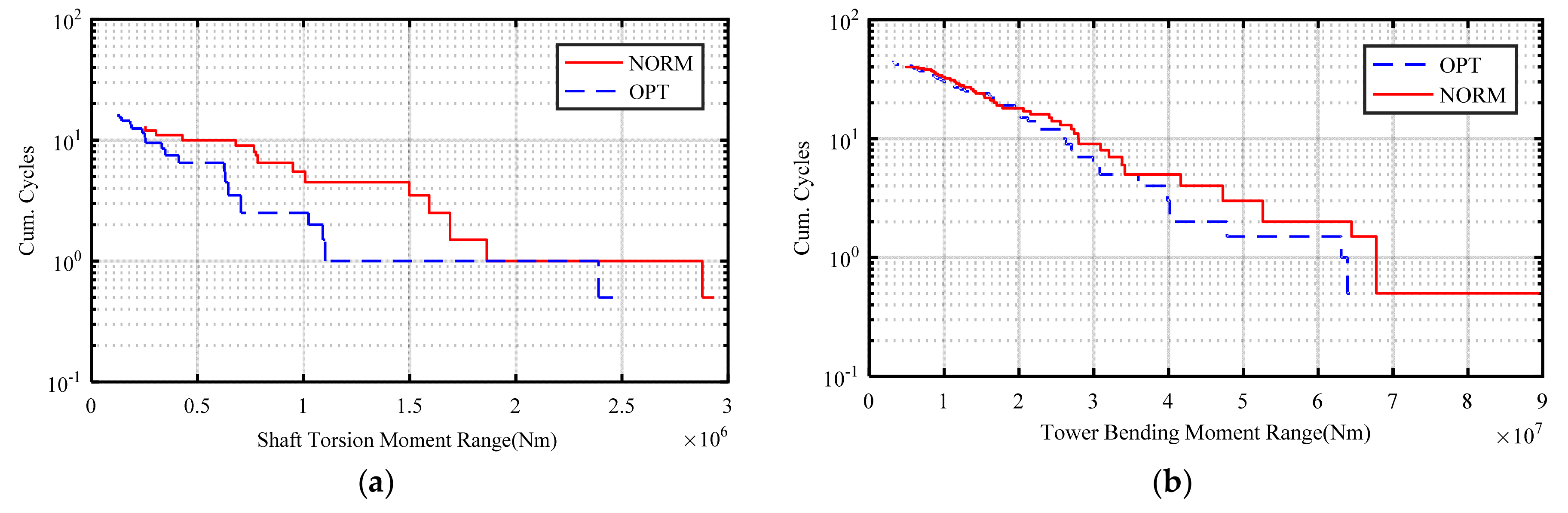
Figure 13.
Total active power and grid frequency response during grid load A. (a) Active power response during grid load A; (b) Grid frequency response during grid load A.
Figure 13.
Total active power and grid frequency response during grid load A. (a) Active power response during grid load A; (b) Grid frequency response during grid load A.
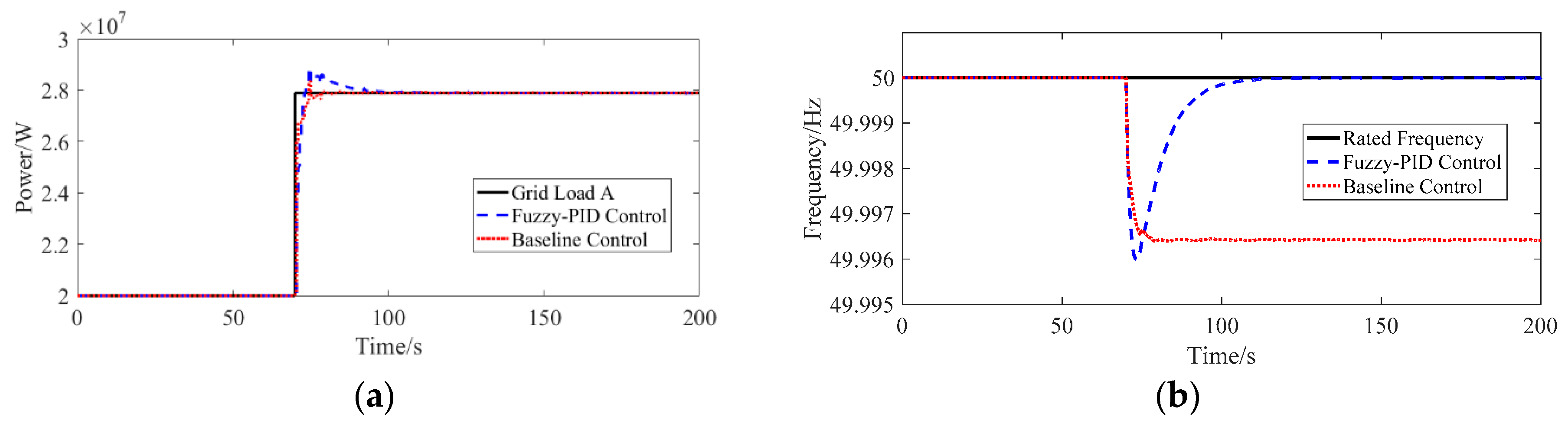
Figure 14.
Total active power and grid frequency response during grid load B. (a) Active power response during grid load B; (b) Grid frequency response during grid load B.
Figure 14.
Total active power and grid frequency response during grid load B. (a) Active power response during grid load B; (b) Grid frequency response during grid load B.

Figure 15.
DELs of the WTs using Baseline Control + NORM, Fuzzy-PID + NORM and Fuzzy-PID + OPT when load B is used to test the overall controller. (a) DELs for Shaft Torsion Moment of the WTs; (b) DELs for Tower Bending Moment of the WTs.
Figure 15.
DELs of the WTs using Baseline Control + NORM, Fuzzy-PID + NORM and Fuzzy-PID + OPT when load B is used to test the overall controller. (a) DELs for Shaft Torsion Moment of the WTs; (b) DELs for Tower Bending Moment of the WTs.


Table 1.
Linguistic variables of membership functions.
| Linguistic Variables | Meaning |
|---|---|
| NB | Negative big |
| NM | Negative medium |
| NS | Negative small |
| Z | Zero |
| PS | Positive small |
| PM | Positive medium |
| PB | Positive big |
Table 2.
Lookup table of Cp (λ, θ).
| λ | λmin | λmin + Δλ | … | λmax | |
|---|---|---|---|---|---|
| θ | |||||
| θmin | 0.0005 | 0.001 | … | −0.8478 | |
| θmin + Δθ | 0.0005 | 0.001 | … | −0.8637 | |
| … | … | … | … | … | |
| θmax | −0.0012 | −0.0036 | … | −207.6793 | |
Table 3.
Parameters of Fuzzy-PID controller.
| Parameter | Value |
|---|---|
| fN | 50 Hz |
| aP | 1 × 10⁸ |
| bP | 3 × 10⁸ |
| aI | 5 × 10⁶ |
| bI | 5 × 10⁷ |
| aD | 5 × 10⁷ |
| bD | 2 × 10⁸ |
Table 4.
Parameters of WT.
| Parameter | Value |
|---|---|
| Rotor inertia: Jr | 3.54 × 10⁷ (kg∙m2) |
| Generator inertia: Jg | 5.34 × 10² (kg∙m2) |
| Gear box ratio: ηg | 97 |
| Filter time constant of ωg: τf | 10 |
| Proportional gain: kp | 0.2143 |
| Integral gain: ki | 0.0918 |
| Gain coefficient: ka1 | 2.1323 |
| Gain coefficient: ka2 | 1 |
| Generator rated speed: ωg-rated | 122.91 (rad/s) |
| Main shaft viscous friction coefficient: B | 6.22 × 10⁶ (Nm∙s/rad) |
| Sir density: ρ | 1.22 (kg/m3) |
| Length of the blade: R | 63 (m) |
| Filter time constant of Tg_ref: τg | 0.1 |
Table 5.
DELs of Ts and Ft for Scenario 1.
| No. | DELs for WTs (Ts/MNm) | DELs for WTs (Mt/MNm) | ||||
|---|---|---|---|---|---|---|
| NORM | OPT | Percentage | NORM | OPT | Percentage | |
| 1 | 1.94 | 2.06 | 6.13% | 50.48 | 44.96 | −10.93% |
| 2 | 1.94 | 1.76 | −9.38% | 57.48 | 57.92 | 0.77% |
| 3 | 1.82 | 1.77 | −2.26% | 62.68 | 60.90 | −2.83% |
| 4 | 1.82 | 1.70 | −6.73% | 54.19 | 47.86 | −11.68% |
| 5 | 1.85 | 2.28 | 23.39% | 42.83 | 40.86 | −4.59% |
| 6 | 1.86 | 1.66 | −11.04% | 59.97 | 58.95 | −1.71% |
| 7 | 1.74 | 1.55 | −10.86% | 65.75 | 64.67 | −1.64% |
| 8 | 1.83 | 1.45 | −20.89% | 48.69 | 40.87 | −16.05% |
| 9 | 1.87 | 2.08 | 11.01% | 42.00 | 38.29 | −8.83% |
| 10 | 1.80 | 1.76 | −2.48% | 58.64 | 58.56 | −0.15% |
| summary | 18.47 | 18.07 | −2.21% | 542.76 | 513.90 | −5.32% |
Table 6.
DELs of Ts and Ft for Scenario 2 and 3.
| Turbulence Intensity | DELs for WTs (Ts/MNm) | DELs for WTs (Mt/MNm) | ||||
|---|---|---|---|---|---|---|
| NORM | OPT | Percentage | NORM | OPT | Percentage | |
| 0.2 | 15.78 | 14.97 | −5.13% | 616.40 | 577.77 | −6.28% |
| 0.3 | 14.63 | 14.27 | −2.46% | 646.93 | 611.33 | −5.50% |
Table 7.
Quantitative comparison of Fuzzy-PID methods in terms of accuracy of response for active power and frequency.
Table 7.
Quantitative comparison of Fuzzy-PID methods in terms of accuracy of response for active power and frequency.
| Control Method | NRMSE for Power Responses | SD for grid Frequency Responses | ||
|---|---|---|---|---|
| Grid Load A | Grid Load B | Grid Load A | Grid Load B | |
| Baseline Control | 0.017545 | 0.104380 | 0.002845 | 0.007423 |
| Fuzzy-PID | 0.021409 | 0.012052 | 0.000764 | 0.001345 |
Table 8.
Total DELs of WTs for three different controllers.
| DELs for WTs (Mt/MNm) | DELs for WTs (Ts/MNm) | |||
|---|---|---|---|---|
| Values | Percentage | Values | Percentage | |
| Baseline Control + NORM | 730.68 | 23.77 | ||
| Fuzzy-PID + NORM | 790.23 | 8.15% | 25.31 | 6.47% |
| Fuzzy-PID + OPT | 733.01 | 0.32% | 24.35 | 2.44% |
© 2019 by the authors. Licensee MDPI, Basel, Switzerland. This article is an open access article distributed under the terms and conditions of the Creative Commons Attribution (CC BY) license (http://creativecommons.org/licenses/by/4.0/).
Share and Cite
MDPI and ACS Style
Liu, Y.; Wang, Y.; Wang, X.; Zhu, J.; Lio, W.H. Active Power Dispatch for Supporting Grid Frequency Regulation in Wind Farms Considering Fatigue Load. Energies 2019, 12, 1508. https://doi.org/10.3390/en12081508
AMA Style
Liu Y, Wang Y, Wang X, Zhu J, Lio WH. Active Power Dispatch for Supporting Grid Frequency Regulation in Wind Farms Considering Fatigue Load. Energies. 2019; 12(8):1508. https://doi.org/10.3390/en12081508
Chicago/Turabian StyleLiu, Yingming, Yingwei Wang, Xiaodong Wang, Jiangsheng Zhu, and Wai Hou Lio. 2019. "Active Power Dispatch for Supporting Grid Frequency Regulation in Wind Farms Considering Fatigue Load" Energies 12, no. 8: 1508. https://doi.org/10.3390/en12081508
Note that from the first issue of 2016, this journal uses article numbers instead of page numbers. See further details here.