Performance of the Stator Winding Fault Diagnosis in Sensorless Induction Motor Drive


Department of Electrical Drives and Measurements, Wrocław University of Science and Technology, 50-370 Wrocław, Poland
*
Author to whom correspondence should be addressed.
Energies 2019, 12(8), 1507; https://doi.org/10.3390/en12081507
Submission received: 22 February 2019
/
Revised: 25 March 2019
/
Accepted: 18 April 2019
/
Published: 21 April 2019
(This article belongs to the Special Issue Condition Monitoring and Diagnosis of Electrical Machines)
Abstract
:This paper deals with the diagnosis of stator winding inter-turn faults for an induction motor drive operating without a speed sensor in a speed-sensorless mode. The rotor direct field oriented control structure (DFOC) was applied, its reference current and voltage component values were analyzed, and their selected harmonics were applied as effective fault indicators. To ensure robust speed estimation, a sliding mode model reference adaptive system (SM-MRAS) estimator was selected. The influence of load torque, reference speed, proportional-integral (PI) controller parameters, and short-circuit current on fault diagnosis and speed estimation performance was verified. Experimental test results obtained for a 3 kW induction motor drive are included.
1. Introduction
Generally, an induction motor (IM) can be supplied from a grid, from a voltage source inverter, or it can be a part of a complex variable speed control structure. The type of the supply has to be taken into account when the diagnostic procedure of the motor is designed [1]. The difference between the closed-loop structure and the remaining supply methods is that fault symptoms in the first and the second cases can only be observed in motor currents. This is the reason why many methods of motor current signature analysis (MCSA) have appeared in the past [2,3,4]. However, in the case of the closed-loop control structure the fault symptoms can be found in both currents and voltage signals [5,6]. Thus, in some cases, the MCSA method is not recommended [2,7,8,9]. Additionally, in the case of the field oriented control (FOC) or the direct torque control (DTC) approaches, fault symptoms can be visible in measured, estimated, and/or reference signals. Although many different diagnostic methods for open-loop or grid-connected motors have appeared [10,11], there is a need to carefully verify closed-loop control structures with IM and the diagnostic methods applied to operate in wide speed and torque ranges.
The diagnostics of stator winding faults for controlled IM is still an open research topic. As shown in [12] there are control structures which, so far, have not ever been analyzed from the point of view of stator winding inter-turn short circuits, e.g., indirect field oriented control (IFOC). A comparison between indirect and direct approaches was made only for rotor-related damages [13].
The diagnosis of stator winding faults was analyzed for three different control structures: DFOC, [9,14,15,16,17,18,19]. DTC with a switching table [8,12], and DTC with space vector modulation (DTC-SVM) [20]. The DFOC and its modifications are the mostly applied in IM control structures, therefore the impact of this control structure has been analyzed most frequently. In [9,15], the second harmonic frequency amplitudes of appropriate signals (currents, voltages) were selected to be the fault symptoms. Additionally, in [15], the influence of the PI controller parameter on the diagnosis performance was analyzed. Instantaneous symmetrical components analysis (ISCA) and principal components analysis (PCA) for both open- and closed-loop controls were compared in [14]. The vibration signals and complex signals analysis [16,17] can be used in the fault diagnosis of the controlled IM as well. Contrary to the above mentioned signal-based methods, the stator resistance estimation by Kalman filter and Luenberger observer [18] and model reference adaptive system (MRAS)-type estimator [19] were applied to diagnose the stator winding faults as well.
The diagnostic methods were also proposed for the DTC structure [8,12,20]. Two different methods, based on the MCSA and multiple reference frame theory, were shown in [8]. The detailed analysis of the inter-turn short circuits influence on the DTC structure was presented in [12]. In [20], authors compared the ISCA of the stator current with the analysis of the second harmonic frequency of internal structure signals for the DTC-SVM. Additionally, this control method was compared to DFOC.
The lack of a speed measurement device included in the drive system allows it to reduce its size, cost, and cabling. Therefore, many speed estimation methods have appeared in the past [21,22]. Yet, this issue is still an interesting scientific problem, especially when the parameter mismatch [23,24] or the regenerating mode operation [25,26,27,28] is taken into account.
There are many different solutions to estimate IM speed. However, in almost all speed estimation technique reviews, the sliding mode (SM) approach is selected to be the most advantageous among various observers, MRAS-type estimators with PI controllers, Kalman Filters, or neural methods [29,30,31,32,33]. It provides the best robustness to parameter variations and system order reduction; it needs a small number of design parameters and is easy to apply in a microprocessor system.
There are different kinds of sliding-mode based speed estimators: Sliding mode observers [34,35], MRAS-type SM estimators [36,37], discrete time estimators [38,39], second order SM estimators [40], and many others. The SM observers are also used to diagnose some IM faults: Broken bars [41], stator inter-turn short-circuits [42,43] inverter transistor faults [44], and speed sensor faults [45].
Although the stability of the estimator during the regenerating mode operation is one of the most important aspects related to the speed estimation, it was carefully analyzed only in a few cases for the sliding mode estimation [27,34]. In this paper, the solution shown in [27] was selected to ensure an accurate and stable speed-sensorless operation under unbalanced stator winding conditions of IM.
The state variables estimator is an important part of the field-oriented control structure, especially when the DFOC is taken into account. It is necessary to determine the rotor flux amplitude, rotor flux angle, and estimated speed. The estimator applied in this paper is an algorithmic estimator that introduces an additional delay in speed determining, on the contrary to modern speed measurement techniques (i.e., incremental encoders). Moreover, the estimator that is based on the mathematical model equations is always dependent on motor parameters mismatch; during the fault the motor becomes an unbalanced system and its resistance differs between the motor phases. Therefore, the fault in stator windings can influence speed estimation and incorrect speed estimation can deteriorate the diagnostic performance. These aspects are verified in this paper. The combination of the stator fault diagnosis and speed estimation has been not analyzed before. Although in [8] authors showed a typical speed-sensorless structure for the DTC control, they did not analyze speed estimation in the case of faulty operation. Despite presenting a block diagram, the authors did not explain whether their drive operates with or without speed measurement. Thus, the objectives of this paper are:
- To verify whether the proposed diagnostic procedure is able to diagnose the faulted stator winding of an induction motor within a sensorless DFOC structure correctly;
- To verify whether a speed estimator is able to estimate speed in the case of stator winding failures.
This paper is divided into six sections. First, the mathematical models of both the healthy induction motor and the speed estimator, which are used to create the sensorless structure, are presented. Then, the rotor field oriented control method for an induction motor is described. Next, the diagnostic procedure is presented, followed by the experimental test results in Section 5. Finally, there is a short conclusion.
2. Mathematical Models
2.1. Mathematical Model of Healthy Induction Motor
The mathematical model of a healthy IM is used to design a speed estimator. It is created using commonly known assumptions (symmetrical structure, lumped windings, constant parameters, neglected eddy currents, no higher harmonics, etc.). It is written in the per unit system (marked with lower case letters; additional time constant TN appears), in stationary reference frame α-β, and with the use of space vector notation (bold font) [46]. It is assumed that the motor is a squirrel-cage star-connected induction motor. The mathematical model consists of [46]:
- Stator and rotor voltage equations:where us = usα + jusβ is the stator voltage space vector, rs is the stator resistance, is = isα + jisβ is the stator current space vector, TN = 1/(2πfsN) is the time constant (only in the per unit system), fsN is the nominal frequency of IM, ψs = ψsα + jψsβ is the stator flux space vector, rr is the rotor resistance, ir = irα + jirβ is the rotor current vector, ψr = ψrα + jψrβ is the rotor flux space vector, and ωm is the mechanical speed.
- Stator and rotor flux equations:where ls = lm + lsσ is the stator winding inductance, lm is the main inductance, lsσ is the stator leakage inductance, lr = lm + lrσ is the rotor winding inductance, and lrσ is the rotor leakage inductance.
- Electromagnetic torque and equation of motion:where te is the electromagnetic torque, tl is the load torque, and TM is the mechanical time constant of the drive.
2.2. Mathematical Model of Eq-SMMRASCC Speed Estimator
The diagnostic procedure is applied within a speed-sensorless control structure, therefore the selected speed estimator is described in this section. Because of its good dynamic performance, robustness over parameter mismatch, and stable operation in the case of the regenerating mode, the sliding mode (SM) model reference adaptive system (MRAS)-type estimator, based on an equivalent (Eq) signal Eq-SMMRASCC [27] will be used in this paper and presented in this section. The superscript CC describes the adaptive part of the MRAS estimator, C is the rotor flux estimation based on a stator current, and C is the stator current estimation. The induction motor is the reference model itself—measured stator currents are compared with the estimated ones. The estimated speed and an auxiliary variable, µ, are introduced to ensure the stable operation of the estimator in the regenerating mode, constituting the vector of estimated variables .
The rotor flux estimation is based on the measured stator current (using modified rotor Equation (2) and Equation (4)):
where ^ indicates estimated value; η = lmrr/lr, τr = rr/lr.
The stator current is estimated as follows (using stator Equation (1) and flux Equation (3) and Equation (4)):
where σ = 1 − lm2/(lslr) is the total leakage factor.
The above Equation (7) and Equation (8) create the adaptive part of the MRAS estimator. The estimated speed and the additional variable are estimated using the following equation [27]:
where
where Kω, Kµ, Mω, Mµ are the positive gains to be selected and sgn is the sign function.
The superscript eq in (10) indicates the equivalent signal—the continuous part of the estimated vector x, calculated using the ideal mathematical model of the IM and the assumption that the switching functions vector s = 0. The superscript d indicates the discontinuous part, used to compensate any possible modeling and parameter mismatch in the equivalent part. The classical SM speed estimators are based only on the discontinuous part in a vast majority of cases. However, gains Mω and Mµ must be large enough to ensure a proper operation of the estimator and they can induce large oscillations (chattering) in estimated variables. In order to reduce this negative phenomenon, some specific techniques must be used, e.g., adaptation of the estimator’s gains [47]. The usage of the equivalent (continuous) part allows a significant reduction of the chattering level, introduced by the sign function in the discontinuous part, in comparison to the classical sliding mode observer [48] and the sliding mode MRAS estimators [37].
Vector f and matrix D in (11) can be calculated after the division of the switching function vector derivative into three parts [27]:
where D is related to the vector of the estimated signals, K is related to the error vector, and f contains the remaining quantities. After a slight simplification, they can be calculated as [27]:
where isα and isβ are the components of the stator current space vector in stationary reference frame obtained using the Clarke transformation from stator phase currents and usα and usβ are the components of the stator voltage space vector; they can be obtained from phase voltages as well or by using the pulse width modulation (PWM) signals and the direct current (DC)-bus voltage uDC.
The objective of the sliding mode algorithm is to ensure the zero value of the sliding mode function vector (12), i.e., s = 0. Simultaneously, functions eω and eμ become zero and the estimated current components are equal to the measured ones (13) under the assumption that , which is always fulfilled in case of field-oriented control.
The use of the auxiliary variable allows stability extension over the regenerating mode, contrary to many different speed estimators unstable in these operation conditions, including SM solutions [48].
Because of the discontinuous part, a low pass filter (LPF) has to be applied if the estimated speed is to be used within the sensorless control structure. The block diagram of the estimator is presented in Figure 1.
3. DFOC Control Structure
The diagnostic method analyzed in this paper and the speed estimator described above both operate under the sensorless direct field oriented control for an induction motor drive [46]. The block diagram of the control structure is presented in Figure 2. The main part of the control scheme consists of four PI controllers to control rotor flux amplitude, speed, and two stator current vector components in the synchronous frame depicted as x-y, rotating with rotor flux vector. The parameters of the PI controllers are shown in Appendix A. The reference rotor flux magnitude is equal to its nominal value or decreased under a field weakening operation when the speed exceeds the nominal value. Reference stator current vector components, the so-called flux-producing component and the torque-producing component, are set by flux and speed controllers, respectively. Reference voltage components, being outputs of PI current controllers, are transformed into the stationary frame α-β and then are used by the space vector modulation (SVM) to ensure the equality of the motor and reference voltages. The outputs of the modulator, kA, kB, and kC, which are the PWM signals together with the DC-bus voltage uDC, are used to calculate the actual voltage values usα and usβ and are used by the speed estimator. In this paper, it is assumed that the field-oriented control operates without taking into account the decoupling signals [9].
In order to perform reference frame transformations, the rotor flux angle signal γψr is necessary; it is estimated by the Eq-SMMRASSCC estimator. This estimator ensures the estimation of the rotor flux amplitude ψr as well, being the feedback signal of the flux PI regulator. The drive operates in a speed-sensorless (or encoderless) structure, which means that its speed is estimated by the presented estimator.
There are several signals from the closed-loop control structure that can be used in the diagnostic procedure: Estimated rotor flux amplitude and angle, estimated speed, reference stator current components, actual current components, and reference voltage signals. The control structure is used to keep the estimated flux and speed equal to their reference values, therefore they are not valuable diagnostic signals. However, the outputs of the speed and flux regulators are modified (in comparison to non-faulty operation) to ensure the required performance of the drive system. Therefore, the reference stator current vector components can be successfully used in the diagnostic procedure, which will be shown in the following section. Similarly, reference voltage signals can be used in the diagnostics as well. The detailed analysis of the diagnostic signals and diagnostic procedure is presented in the following sections.
4. Diagnostic Procedure
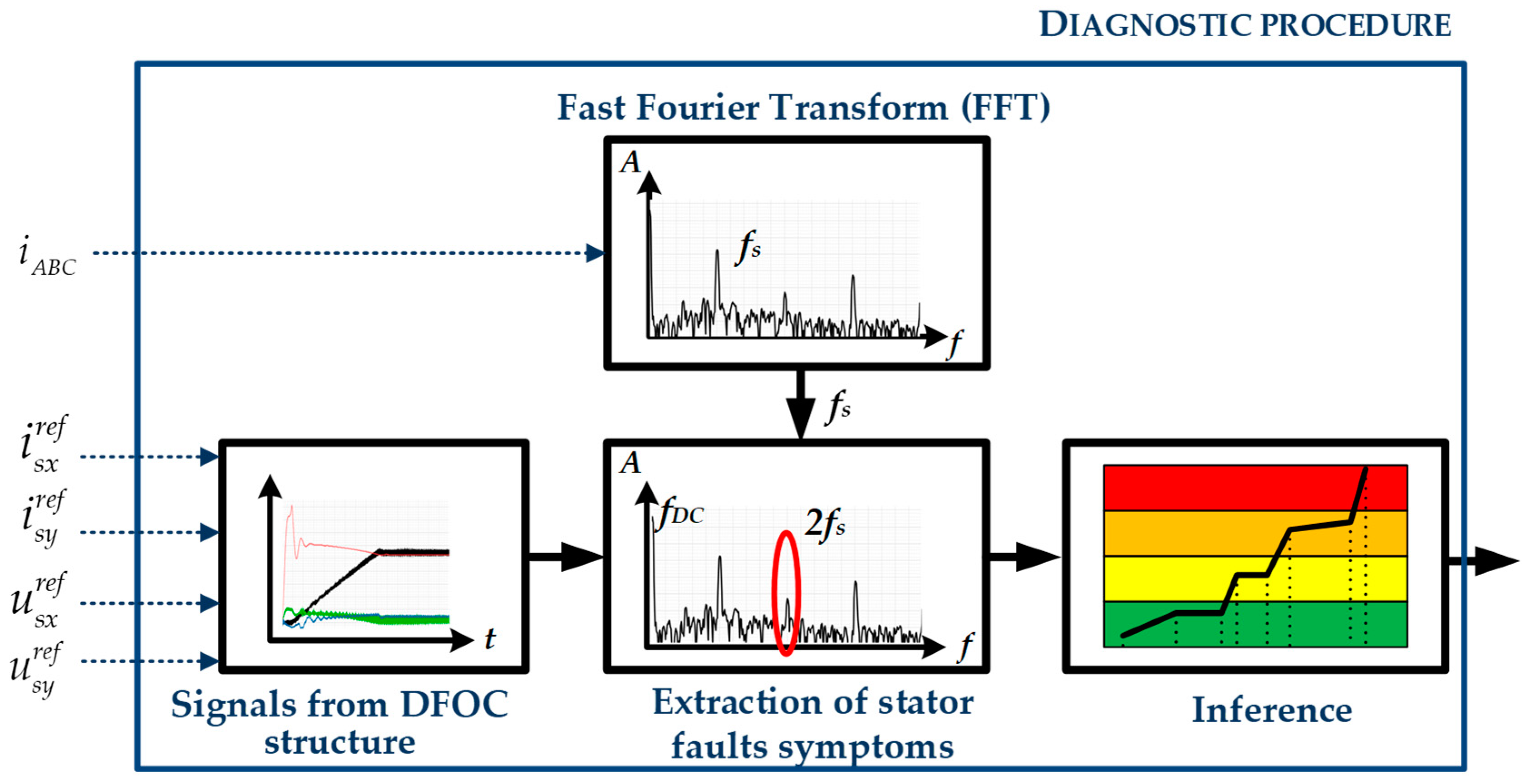
The proposed diagnostic procedure for a sensorless DFOC induction motor drive is shown in Figure 3. It is similar to the procedure presented in [9], however, the diagnostic signals used in this paper are different. Additionally, the control structure operates without a speed sensor and control paths decoupling. The diagnostic procedure can be described using the following steps:
- Identification of the fundamental frequency fs of induction motor supply voltages or currents. In this paper, the phase currents are used to determine the frequency, as shown in Figure 2—the currents have to be measured in the DFOC structure. However, measured stator voltage or calculated voltage vector components usα and usβ can be used as well. The identification is made using the fast Fourier transform (FFT) with a selected window (flat-top in this paper). Because of this, the diagnostic procedure must be conducted during a steady-state, while the motor speed is constant.
- Extraction of four reference signals from the control structure; reference stator current vector components and reference voltage vector components.
- Determination of the 2fs harmonics frequency amplitudes for all diagnostic signals. These amplitudes will be used further as fault symptoms.
- Depending on the determined values of fault symptoms, an inference is drawn regarding whether the motor is healthy or not. It can be based on a predefined threshold. In the case of an industrial inverter, the threshold can be determined during the commissioning stage, i.e., during the identification procedure of motor parameters (this is a standard procedure in the case of all modern voltage source inverters (VSIs) applied in the industry, where the vector control method is used). In this case, the threshold can be set as the maximum value of the second harmonic amplitude for all of the diagnostic signals. Unfortunately, their values depend slightly on motor speed and load torque, therefore the threshold should be increased suitably so as not to generate false alarms. This dependence will be shown in the subsequent sections.
5. Description of the Experimental Set-up
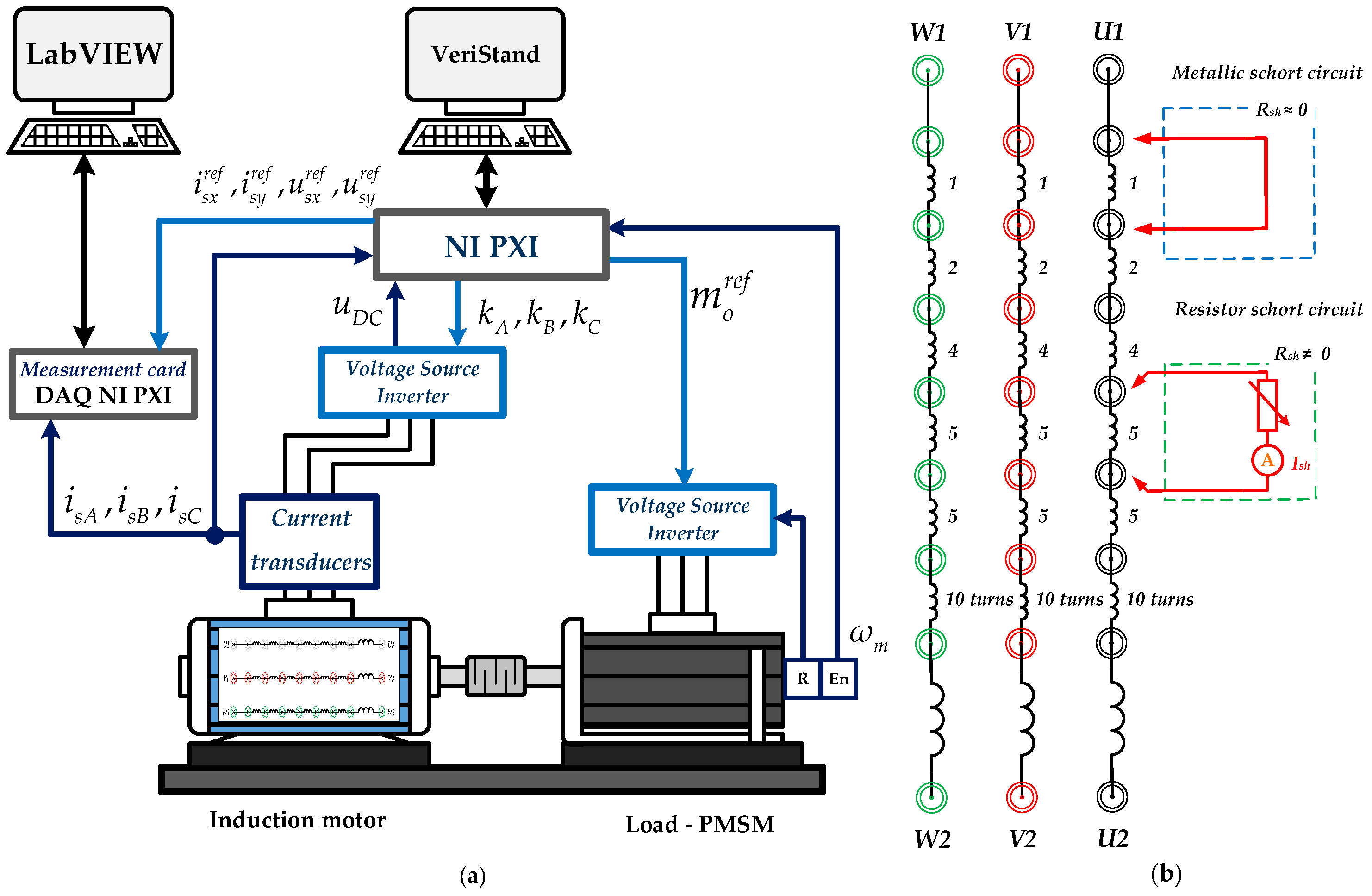
A block diagram of the experimental setup is shown in Figure 4a. The main part of the experimental setup is a 3 kW induction motor, specially modified (rewound) to allow the modeling of short circuits in all three phases, as shown in Figure 4b. The induction motor allows the modeling of a short circuit using a metallic connection or the inclusion of an additional resistance Rsh and the measurement of the Ish current by an ammeter. As shown in Figure 4b, it is possible to model the short-circuit of 1, 2, 4, 5, 8, and 10 turns in each phase of the machine. In order to obtain different numbers of short-circuit turns, a combination of the above can be used (e.g., to obtain three short-circuit turns, one plus two turns can be a short-circuit simultaneously). The photograph of the experimental setup is shown in Figure 5.
The parameters and the nominal data of the IM, used during the experiments, are shown in the Appendix A and Appendix B. IM is supplied by a voltage source inverter (VSI) that allows controlling of its switches using fiber-optic wires. The VSI is controlled with 10 kHz frequency by a modular rapid prototyping system, NI Peripheral component interconnect eXtensions for instrumentation (PXI) by National Instruments (NI), equipped with an field-programmable gate array (FPGA) card and a real-time system. Three phase currents and the DC-bus voltage are measured to perform control, estimation, and PWM modulation algorithms.
The PXI defines the load torque value and sends it to another VSI that supplies a permanent magnet synchronous servo motor. The PMSM is extended with a resolver and an incremental encoder to determine speed and the shaft angle. The speed is measured only for comparison purposes; the diagnostic procedure effectiveness will be compared between the sensor and sensorless operations.
In order to perform the diagnostic procedure, the reference signals form the control structure where currents and voltages are sent from one PXI to another as analogue signals, which are measured by a data acquisition (DAQ) measurement card. This cooperation is made only to divide control and diagnostic algorithms. In the case of an industrial inverter application, the diagnostic procedure can be easily applied together with control and estimation algorithms.
The influence of the short circuit current on the diagnostic signal value is verified in Figure 6 for five shorted turns in phase A. As can be seen, in order to limit the current of the short circuit, additional resistance can be used (for Rsh = 0 Ω, Ish ≈ 28 A). Short-circuit resistance grows along with a decrease in the short-circuit current. Moreover, it can be seen that the dependence of the diagnostic signals (both current and voltage) on the short-circuit current value is approximately linear. Thus, inferring about the motor condition and the quality of the diagnostic process can be significantly reduced (difficult) if the short-circuit is not metallic. However, when the current in the short-circuit circuit is relatively small, the damage is not so dangerous for the machine.
The following subchapters include the detailed analysis of both sensorless control structure and the diagnosis algorithm performance in the case of a non-faulty and faulty operation, with various speeds and load torques.
6. Experimental Verification
6.1. Sensorless Control in Case of non-Faulty Operation
The performance of the Eq-SMMRASCC estimator within a fully sensorless DFOC structure, in the case of a non-faulty operation, is shown in Figure 7. It can be seen in Figure 7a that the estimated speed follows the real speed and the reference speed precisely, with a very small delay. The estimated speed consists of two parts: A discontinuous and continuous (equivalent) one, which are both shown in Figure 7b. It can be seen that the equivalent signal (blue) follows the real speed, however, its average value after filtration would be different than the mechanical speed. It can be caused by the parameter mismatch, discrete realization of the control structure, modified structure of the motor (to allow short-circuits of stator winding), non-ideal estimation of stator voltage, noise intensified by the derivatives of current components in (14), etc. Therefore, the estimator is extended with the discontinuous signal (black in Figure 7b) to compensate for possible imperfections. The sum of the two mentioned signals is filtered to create the final form of the estimated signal, shown in Figure 7a.
As can be seen, the speed is controlled perfectly in the sensorless structure. Similarly, the rotor flux amplitude (Figure 7c) is kept at its reference, nominal level. The speed switching function is shown in Figure 7d, which proves that the objective of the estimator (zero value of the switching function s) is ensured. The current components are estimated quite well, as shown in Figure 7e. The biggest estimation error appears during the reversions.
6.2. On-line Speed Estimation and Fault Diagnosis
The objective of this paper is to evaluate the possibility of estimating the speed in the case of the stator inter-turn faults and vice versa, to evaluate the diagnostic procedure of the stator winding in the case of speed-sensorless operation. Both of these are presented in Figure 8. The test presents constant speed operation in the case of the fault increasing level—the number of short-circuit turns in phase A of the motor increases every five seconds, as shown in Figure 8b, from one to eight short-circuit turns. The presented results are shown for the no-resistance case. All of the diagnostic signals are presented here in relation to their values in the case of healthy operation (Nsh = 0).
Figure 8a shows encoderless operation; the estimated speed (black) oscillates around the reference value (red, 80% of nominal speed). It can be seen that the speed estimation is almost perfect, even in the case of stator winding fault diagnosis (Figure 8a). Due to the asymmetry introduced by the faulted winding the oscillation level of both estimated and real speed increases together with raising Nsh, however, the oscillations can be practically neglected in comparison to the actual speed signal.
The online waveforms of the diagnostic signals are shown in Figure 8c–f. According to the diagnostic procedure described above, the online algorithm first determines the fundamental frequency fs of phase currents and then calculates the 2fs frequency amplitudes of all four fault indicators. Each analyzed diagnostic signal is shown in Figure 8c–f: Reference stator current and voltage space vector components, respectively. It can be seen that the amplitudes of the second harmonics increase successively for all signals under consideration. In fact, the short circuit of only one turn is almost invisible. However, two short-circuit turns give a noticeable change of the amplitude (only the reference usy varies not significantly). Although the absolute values of the signals are small, the relative changes referred to the healthy values are significant. Definitely, the x-axis components (current and voltage), connected with the rotor flux amplitude regulation, are more sensitive to occurring damage. Their usage in the fault diagnosis is preferable in comparison to the second (torque) control path, including y-axis components.
6.3. FFT Analysis of the Diagnostic Signals Under Sensorless Operation
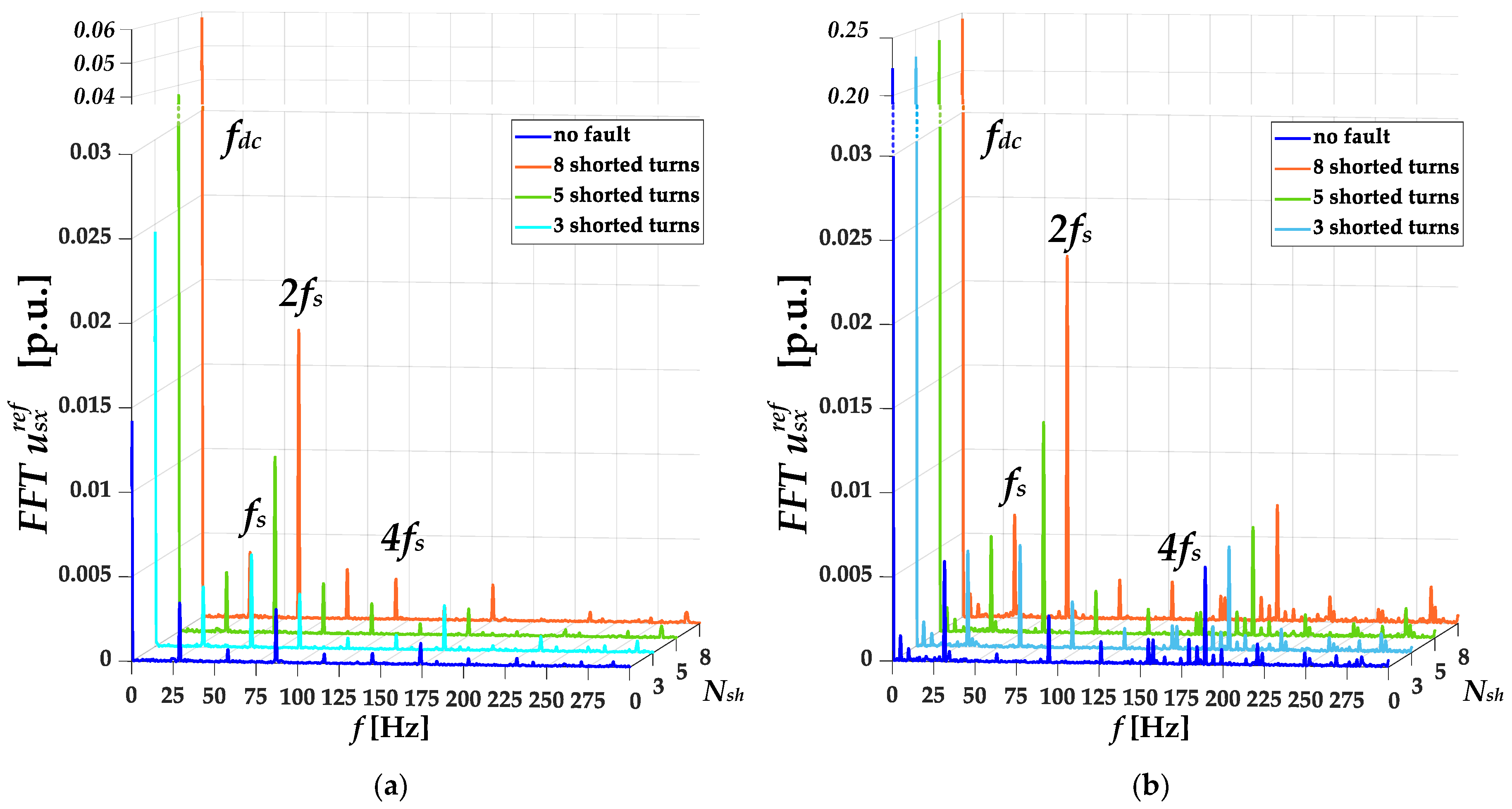
The FFT of the field-producing current is shown in Figure 9 for idle running (Figure 9a) and the operation with a nominal load (Figure 9b). The analysis is shown for various numbers of short-circuit turns.
Due to the nature of the DFOC and its similarity to the DC motor control, the analyzed signals should be generally constant in time when the speed and the load torque are constant. The amplitude of the rotor flux should be constant, therefore the flux-producing current isx should be constant as well. Consequently, due to the constant speed, the motor torque, proportional to isy, should be constant and equal to constant load torque. Therefore, all signals contain the DC component and the amplitude of the fdc component is large and much higher than the diagnostic signals analyzed in this paper.
Except for the DC components, there are still some frequencies that can be observed in the reference x-axis current component: The fundamental supply voltage frequency fs, its multiples kfs, and the frequencies related to the slip speed (only in the case of the load torque presence, Figure 9b). The remaining frequencies are practically invisible and can be neglected in the analysis. As can be seen, the fs, 3fs, 5fs, and 6fs frequencies and the slip frequencies are independent of the level of the stator winding damage and cannot be treated as the indicators of the fault. On the other hand, only the amplitudes of 2fs and 4fs frequencies vary with the number of short-circuit turns and can be used in the diagnostic process. As was stated in Section 4, due to the highest sensitivity to the stator winding failure, the 2fs frequency amplitude is selected to be the fault indicator.
Figure 10 shows an analysis similar to the one presented in Figure 9, however, this time it is related to the reference x-axis voltage component for no-load operation (Figure 10a) and the operation with nominal load torque (Figure 10b). The conclusions are analogical to the previous ones; the 2fs frequency from the FFT analysis is the most valuable diagnostic signal.
6.4. Influence of Load Torque and Motor Speed on the Effectiveness of the Diagnostic Procedure
Figure 11 shows the influence of the load torque on the performance of the diagnostic procedure using the magnitudes of the characteristic frequency harmonic fsh = 2fs of the reference flux-producing current isx. Additionally, it shows the comparison between the operation with speed measurement (Figure 11a) and the sensorless operation (Figure 11b). The tests are presented for nine different numbers of short-circuit turns and six different values of the load torque. It can be seen that the amplitude of the second harmonic frequency is almost independent of the load torque value, which is very important under fault diagnosis. In all cases the amplitude increases monotonically with rising Nsh. This effect is similar in both cases, with and without speed measurement. However, the values of the diagnostic signal are larger in the case of the sensorless control structure. A more detailed comparison of both control modes is shown in Section 6.5.
On the other hand, Figure 12 presents the influence of motor speed on the second harmonic frequency of the reference x-axis stator current in the case of constant load torque. The dependence of the diagnostic signals is now stronger and changes relatively more than in the case of varying load torque and constant rotor speed. Additionally, the trends are entirely different between speed sensor usage (Figure 12a) and sensorless operation (Figure 12b). For the speed measurement, the diagnostic index decreases with the speed value, while in the case of sensorless operation this index increases. However, its value is still much bigger than in a non-faulty situation (Nsh = 0). Additionally, it proves that the value of the diagnostic signal cannot be taken directly as an indicator of the number of short-circuit turns (e.g., the value of 0.008 can indicate four short-circuit turns in the case of nominal speed and eight short-circuit turns for 0.2 ωmN). However, it can still be taken as an input of some neural-network based fault detector or used to determine the trend of the fault signature in time.
Figure 13 and Figure 14 are analogical to Figure 11 and Figure 12, while the analysis is related now to the reference x-axis voltage vector component. The obtained results are similar when the speed is constant and the influence of the load torque value is minimal. However, the influence of the rotor speed value on the diagnostic signal magnitudes is strong and changes monotonically in both cases, speed-sensor and speed-sensorless operations. The higher the speed, the bigger the diagnostic signal value. It proves once again that the diagnosis of stator windings is more effective for higher speed values than for a low speed range.
6.5. The Difference Between Sensorless Operation and Speed Sensor Usage
Figure 15 shows the comparison between the sensorless operation and the operation with a speed sensor for five short-circuit turns of the stator winding and for a healthy motor case (blue planes). Field-producing current (Figure 15a) and voltage (Figure 15b) are compared as well. The opposite tendency of a decreasing (sensor operation—light green) and increasing (sensorless operation—bottle green) diagnostic signal can be now clearly seen in reference stator current component isx (Figure 15a). These results are strictly connected with the data shown in Figure 12. However, the diagnostic signal in both cases is much bigger for the damaged (green color) than for undamaged motor (blue color). In contrast to this, the diagnostic signals in the case of the analyzed voltage component usx (Figure 15b) for both sensor and sensorless operations are very similar; the tendency is identical.
6.6. Influence of the PI Controller Parameters on the Diagnostic Procedure
Finally, the influence of the PI controller parameters of the DFOC structure on the diagnostics performance is verified. Values of the controller parameters used in all preceding tests are shown in Appendix A. The form of the transfer function of the PI controllers used in this paper is as follows:
where Kp is the controller gain, Ti is the integral time constant of the controller, and p is the Laplace transform variable.
According the analysis performed in previous sections, the detailed verification is made for two controllers: The rotor flux and field-producing current controllers. It is shown in Figure 16. All the tests are made for increasing number of shorted turns, i.e., Nsh = 2, 4, 6, 8. Two different scenarios are evaluated:
Both proposed fault indicators, i.e., the 2fs frequency amplitudes of reference isx and usx are presented in Figure 16a–d, respectively. It can be seen that the parameters of the PI controllers have an impact only on the current component. Its sensitivity to stator winding faults increases when the flux controller parameters are increased. On the other hand, the sensitivity decreases when the isx controller parameters are increased. Nevertheless, the fault indicator related to motor voltage remains almost constant in all presented situations. Hence, the 2fs frequency harmonics of the reference voltage component seems to be a more effective and reliable fault indicator.
7. Conclusions
This paper presents the stator windings short-circuit diagnostic method for a sensorless vector-controlled induction motor. The direct field oriented control is applied to control the motor effectively and precisely. The outputs of all four PI controllers used in the control structure are considered as fault indicators. Two of them, i.e., the reference field-producing current component and the field-producing voltage component were proven to be more fault sensitive than torque-producing components and are subject to further analysis.
It was shown that the second harmonic frequency of these signals can be selected as a diagnostic indicator. It increased together with an increase in the number of shorted turns. Simultaneously, the influence of the current in the short circuit, load torque, and motor speed on the diagnostic procedure was verified and compared. It was proven that the load torque value has almost no impact on the selected diagnostic symptoms. However, the low speed of the motor decreased the sensitivity of the diagnostic method, therefore the fault diagnosis should be conducted for higher speeds of the machine. The speed has to be constant as well, to allow proper operation of the FFT algorithm.
Moreover, the influence of the PI controller parameters on the stator winding diagnostics was presented. It was shown that the stator voltage component related to the rotor flux control is superior over the current component. This is due to its almost full independence on the controller parameter values.
This paper shows that the speed estimation using the equivalent signal-based sliding mode MRAS estimator allows the obtainment of a precise and effective speed estimation, not only in the unfaulty condition, but also robust to the stator winding fault occurrence. On the other hand, the diagnostic procedure can be successfully applied in both sensorless and sensor-based operations.
Author Contributions
Investigation, G.T. and M.W.; methodology, G.T. and M.W.; validation, G.T.; visualization, M.W.; writing—original draft, G.T. and M.W.
Funding
This research was supported by statutory funds of the Faculty of Electrical Engineering of the Wroclaw University of Science and Technology (2018-2019).
Conflicts of Interest
The authors declare no conflict of interest.
Appendix A
Nominal parameters of PI controllers are shown in Table A1.

Table A1.
Parameters of PI controllers.
| Controlled Variable | Kp | Ti |
|---|---|---|
| Speed | Kp_ω = 3 | Ti_ ω= 0.05 s |
| Rotor flux amplitude | Kp_ψ = 6 | Ti_ ψ= 0.01 s |
| Torque-producing current component | Kp_isx = 1 | Ti_ isx= 0.01 s |
| Field-producing current component | Kp_isy = 1 | Ti_ isy= 0.01 s |
Appendix B
Nominal data and parameters of tested induction motor are shown in Table A2.
Table A2.
Nominal parameters of tested induction machine.
| Name | Symbol | SI Units | Normalized Units [p.u.] | |
|---|---|---|---|---|
| Power | PN | 3000 | [W] | 0.6394 |
| Speed | NN | 1445 | [r/min] | 0.963 |
| Stator phase voltage | UsN | 400 | [V] | 0.707 |
| Stator current | IsN | 6.8 | [A] | 0.707 |
| Frequency | fsN | 50 | [Hz] | 1 |
| Rotor flux | ψrN | 0.927 | [Wb] | 0.895 |
| Torque | TlN | 19.83 | [Nm] | 0.664 |
| Pole pairs | pp | 2 | - | - |
| Stator resistance | Rs | 1.768 | [Ω] | 0.0523 |
| Rotor resistance | Rr | 1.4970 | [Ω] | 0.0443 |
| Main inductance | Lm | 181.5 | [mH] | 1.6858 |
| Stator leakage inductance | Lsσ | 8.9 | [mH] | 0.0827 |
| Rotor leakage inductance | Lrσ | 8.9 | [mH] | 0.0827 |
| Number of stator turns | Ns | 3x180 | [-] | [-] |
References
- Cheng, S.; Zhang, P.; Habetler, T.G. An Impedance Identification Approach to Sensitive Detection and Location of Stator Turn-to-Turn Faults in a Closed-Loop Multiple-Motor Drive. IEEE Trans. Ind. Electron. 2011, 58, 1545–1554. [Google Scholar] [CrossRef]
- Merizalde, Y.; Hernández-Callejo, L.; Duque-Perez, O. State of the art and trends in the monitoring, detection and diagnosis of failures in electric induction motors. Energies 2017, 10, 1056. [Google Scholar] [CrossRef]
- Henao, H.; Capolino, G.; Fernandez-Cabanas, M.; Filippetti, F.; Bruzzese, C.; Strangas, E.; Pusca, R.; Estima, J.; Riera-Guasp, M.; Hedayati-Kia, S. Trends in Fault Diagnosis for Electrical Machines: A Review of Diagnostic Techniques. IEEE Ind. Electron. Mag. 2014, 8, 31–42. [Google Scholar] [CrossRef]
- Wolkiewicz, M.; Kowalski, C.T. Incipient stator fault detector based on neural networks end symmetrical components analysis for induction motor drives. In Proceedings of the 13th Selected Issues of Electrical Engineering and Electronics (WZEE), Rzeszow, Poland, 4–8 May 2016; pp. 1–7. [Google Scholar] [CrossRef]
- Tallam, R.M.; Lee, S.B.; Stone, G.C.; Kliman, G.B.; Yoo, J.; Habetler, T.G.; Harley, R.G. A survey of methods for detection of stator-related faults in induction machines. IEEE Trans. Ind. Appl. 2007, 43, 920–933. [Google Scholar] [CrossRef]
- Tallam, R.M.; Habetler, T.G.; Harley, R.G. Stator winding turn-fault for closed-loop induction motor drives. IEEE Trans. Ind. Appl. 2003, 39, 720–724. [Google Scholar] [CrossRef]
- Maraaba, L.; Al-Hamouz, Z.; Abido, M. An efficient stator inter-turn fault diagnosis tool for induction motors. Energies 2018, 11, 653. [Google Scholar] [CrossRef]
- Cruz, S.M.A.; Cardoso, A.J.M. Diagnosis of stator inter-turn short circuits in DTC induction motor drives. IEEE Trans. Ind. Appl. 2004, 40, 1349–1360. [Google Scholar] [CrossRef]
- Wolkiewicz, M.; Tarchała, G.; Orłowska-Kowalska, T.; Kowalski, C.T. Online Stator Interturn Short Circuits Monitoring in the DFOC Induction-Motor Drive. IEEE Trans. Ind. Electron. 2016, 63, 2517–2528. [Google Scholar] [CrossRef]
- Nandi, S.; Toliyat, H.A.; Li, X. Condition monitoring and fault diagnosis of electrical motors—A review. IEEE Trans. Energy Convers. 2005, 20, 719–729. [Google Scholar] [CrossRef]
- Singh, G. Induction machine drive condition monitoring and diagnostic research—A survey. Electr. Power Syst. Res. 2003, 64, 145–158. [Google Scholar] [CrossRef]
- Berzoy, A.; Mohammed, O.A.; Restrepo, J. Analysis of the Impact of Stator Interturn Short-Circuit Faults on Induction Machines Driven by Direct Torque Control. IEEE Trans. Energy Convers. 2018, 33, 1463–1474. [Google Scholar] [CrossRef]
- Cruz, S.M.A.; Cardoso, A.J.M. Diagnosis of rotor faults in direct and indirect FOC induction motor drives. In Proceedings of the 2007 European Conference on Power Electronics and Applications, Aalborg, Denmark, 2–5 September 2007; pp. 284–293. [Google Scholar] [CrossRef]
- Wolkiewicz, M.; Tarchała, G.; Kowalski, C.T. Stator windings condition diagnosis of voltage inverter-fed induction motor in open and closed-loop control structures. Arch. Electr. Eng. 2015, 64, 67–79. [Google Scholar] [CrossRef]
- Bellini, A.; Filippetti, F.; Franceschini, G.; Tassoni, C. Closed-loop control impact on the diagnosis of induction motors faults. IEEE Trans. Ind. Appl. 2000, 36, 1318–1329. [Google Scholar] [CrossRef]
- Seshadrinath, J.; Singh, B.; Panigrahi, B.K. Investigation of Vibration Signatures for Multiple Fault Diagnosis in Variable Frequency Drives Using Complex Wavelets. IEEE Trans. Power Electron. 2014, 29, 936–945. [Google Scholar] [CrossRef]
- Seshadrinath, J.; Singh, B.; Panigrahi, B.K. Vibration Analysis Based Interturn Fault Diagnosis in Induction Machines. IEEE Trans. Ind. Inform. 2014, 10, 340–350. [Google Scholar] [CrossRef]
- Kowalski, C.T.; Wierzbicki, R.; Wolkiewicz, M. Stator and Rotor Faults Monitoring of the Inverter-Fed Induction Motor Drive using State Estimators. Automatika 2013, 54, 348–355. [Google Scholar] [CrossRef]
- Bednarz, S.A.; Dybkowski, M.; Wolkiewicz, M. Identification of the Stator Faults in the Induction Motor Drives Using Parameter Estimator. In Proceedings of the 18th IEEE International Power Electronics and Motion Control Conference (PEMC), Budapest, Hungary, 26–30 August 2018; pp. 688–693. [Google Scholar] [CrossRef]
- Wolkiewicz, M.; Tarchała, G.; Orlowska-Kowalska, T.; Kowalski, C. Stator fault monitoring based on internal signals of vector controlled induction motor drives. In Proceedings of the 42nd Annu. Conf. IEEE Ind. Electron. Soc. (IECON), Florence, Italy, 23–26 October 2016; pp. 2651–2656. [Google Scholar] [CrossRef]
- Pacas, M. Sensorless Drives in Industrial Applications. IEEE Ind. Electron. Mag. 2011, 5, 16–23. [Google Scholar] [CrossRef]
- Kumar, R.; Das, S.; Syam, P.; Chattopadhyay, A.K. Review on model reference adaptive system for sensorless vector control of induction motor drives. IET Electr. Power Appl. 2015, 9, 496–511. [Google Scholar] [CrossRef]
- Kandoussi, Z.; Boulghasoul, Z.; Elbacha, A.; Tajer, A. Sensorless control of induction motor drives using an improved MRAS observer. J. Electr. Eng. Technol. 2017, 12, 1456–1470. [Google Scholar] [CrossRef]
- Chen, B.; Yao, W.; Chen, F.; Lu, Z. Parameter Sensitivity in Sensorless Induction Motor Drives With the Adaptive Full-Order Observer. IEEE Trans. Ind. Electron. 2015, 62, 4307–4318. [Google Scholar] [CrossRef]
- Etien, E.; Chaigne, C.; Bensiali, N. On the stability of full adaptive observer for induction motor in regenerating mode. IEEE Trans. Ind. Electron. 2010, 57, 1599–1608. [Google Scholar] [CrossRef]
- Harnefors, L.; Hinkkanen, M. Complete stability of reduced-order and full-order observers for sensorless IM drives. IEEE Trans. Ind. Electron. 2008, 55, 1319–1329. [Google Scholar] [CrossRef]
- Tarchała, G.; Orłowska-Kowalska, T. Equivalent-Signal-Based Sliding Mode Speed MRAS-Type Estimator for Induction Motor Drive Stable in the Regenerating Mode. IEEE Trans. Ind. Electron. 2018, 65, 6936–6947. [Google Scholar] [CrossRef]
- Korzonek, M.; Orłowska-Kowalska, T. Comparative Stability Analysis of Stator Current Error-Based Estimators of the Induction Motor Speed. Power Electron. Drives 2018, 3, 187–203. [Google Scholar] [CrossRef]
- Lin, F.J.; Wai, R.J.; Kuo, R.H.; Liu, D.C. A comparative study of sliding mode and model reference adaptive speed observers for induction motor drive. Electr. Power Syst. Res. 1998, 44, 163–174. [Google Scholar] [CrossRef]
- Chen, F.; Dunnigan, M.W. Comparative study of a Sliding-Mode Observer and Kalman filters for full state estimation in an induction machine. IEE Proc.-Elect. Power Appl. 2002, 149, 53–64. [Google Scholar] [CrossRef]
- Zhang, Y.; Zhao, Z.; Lu, T.; Yuan, L.; Xu, W.; Zhu, J. A comparative study of Luenberger Observer, Sliding Mode Observer and Extended Kalman Filter for sensorless vector control of induction motor drives. In Proceedings of the IEEE Energy Conversion Congress and Exposition (ECCE), San Jose, CA, USA, 20–24 September 2009; pp. 2466–2473. [Google Scholar] [CrossRef]
- Khater, M.M.; Zaky, M.S.; Yasin, H.; Shokralla, S.S.; Ei-Sabbe, A. A comparative study of sliding mode and Model Reference Adaptive Speed observers for induction motor drives. In Proceedings of the 11th International Middle East Power Systems Conference (MEPCON), El-Minia, Egypt, 19–21 December 2006; pp. 434–440. [Google Scholar]
- Sutnar, Z.; Peroutka, Z.; Rodič, M. Comparison of Sliding Mode Observer and Extended Kalman Filter for Sensorless DTC-Controlled Induction Motor Drive. In Proceedings of the 14th International Power Electronics and Motion Control Conference (EPE-PEMC), Ohrid, Macedonia, 6–8 September 2010; pp. 55–62. [Google Scholar] [CrossRef]
- Hamajima, T.; Hasegawa, M.; Doki, S.; Okuma, S. Sensorless Vector Control of Induction Motor Stabilized at the Whole Region with Speed and Stator Resistance Identification based on Augmented Error. IEEJ Trans. Ind. Appl. 2006, 155, 52–63. [Google Scholar] [CrossRef]
- Doki, S.; Sangwongwanich, S.; Okuma, S. Implementation of speed-sensor-less field-oriented vector control using adaptive sliding observer. In Proceedings of the International Conference on Industrial Electronics, Control, Instrumentation, and Automation (IECON), San Diego, CA, USA, 13 November 1992; pp. 453–458. [Google Scholar] [CrossRef]
- Gadoue, S.M.; Giaouris, D.; Finch, J.W. MRAS Sensorless Vector Control of an Induction Motor Using New Sliding-Mode and Fuzzy-Logic Adaptation Mechanisms. IEEE Trans. Energy Convers. 2010, 25, 394–402. [Google Scholar] [CrossRef]
- Comanescu, M.; Xu, L.Y. Sliding-mode MRAS speed estimators for sensorless vector control of induction machine. IEEE Trans. Ind. Electron. 2006, 53, 146–153. [Google Scholar] [CrossRef]
- Vieira, R.P.; Gastaldini, C.C.; Azzolin, R.Z.; Gründling, H.A. Discrete-time sliding mode speed observer for sensorless control of induction motor drives. IET Electr. Power Appl. 2012, 6, 681–688. [Google Scholar] [CrossRef]
- Vieira, R.P.; Gabbi, T.S.; Grundling, H. Combined Discrete-time Sliding Mode and Disturbance Observer for Current Control of Induction Motors. J. Control Autom. Electr. Syst. 2017, 28, 380–388. [Google Scholar] [CrossRef]
- Zhao, L.H.; Huang, J.; Liu, H.; Li, B.N.; Kong, W.B. Second-Order Sliding-Mode Observer With Online Parameter Identification for Sensorless Induction Motor Drives. IEEE Trans. Ind. Electron. 2014, 61, 5280–5289. [Google Scholar] [CrossRef]
- Baccarini, L.M.R.; Tavares, J.P.B.; de Menezes, B.R.; Caminhas, W.M. Sliding mode observer for on-line broken rotor bar detection. Electr. Power Syst. Res. 2010, 80, 1089–1095. [Google Scholar] [CrossRef]
- Sellami, T.; Berriri, H.; Jelassi, S.; Mimouni, M.F. Sliding Mode Observer-Based Fault-Detection of Inter-Turn Short-Circuit in Induction Motor. In Proceedings of the 14th International Conference on Electrical Engineering, Computing Science and Automatic Control (STA), Sousse, Tunisia, 20–22 December 2013; pp. 524–529. [Google Scholar] [CrossRef]
- Sellami, T.; Berriri, H.; Jelassi, S.; Darcherif, A.M.; Mimouni, M.F. Short-Circuit Fault Tolerant Control of a Wind Turbine Driven Induction Generator Based on Sliding Mode Observers. Energies 2017, 10, 1611. [Google Scholar] [CrossRef]
- Maamouri, R.; Trabelsi, M.; Boussak, M.; M’Sahli, F. A sliding mode observer for inverter open-switch fault diagnostic in sensorless induction motor drive. In Proceedings of the 42nd Annual Conference of the IEEE Industrial Electronics Society (IECON), Florence, Italy, 23–26 October 2016; pp. 2153–2158. [Google Scholar] [CrossRef]
- Kommuri, S.K.; Rath, J.J.; Veluvolu, K.C.; Defoort, M.; Soh, Y.C. Decoupled current control and sensor fault detection with second-order sliding mode for induction motor. IET Control Theory Appl. 2015, 9, 608–617. [Google Scholar] [CrossRef]
- Kaźmierkowski, M.; Krishnan, R.; Blaabjerg, F. Control in Power Electronics—Selected Problems; Academic Press—An imprint of Elsevier Science: San Diego, CA, USA, 2002; p. 250. [Google Scholar]
- Tarchała, G. Influence of the sign function approximation form on performance of the sliding-mode speed observer for induction motor drive. In Proceedings of the International Symposium on Industrial Electronics, Gdańsk, Poland, 27–30 June 2011; pp. 1397–1402. [Google Scholar] [CrossRef]
- Yan, Z.; Jin, C.X.; Utkin, V.I. Sensorless sliding-mode control of induction motors. IEEE Trans. Ind. Electron. 2000, 47, 1286–1297. [Google Scholar] [CrossRef]
Figure 1.
Block diagram of the applied speed estimator Eq-SMMRASCC [27]. IM: induction motor, LPF: low pass filter.
Figure 1.
Block diagram of the applied speed estimator Eq-SMMRASCC [27]. IM: induction motor, LPF: low pass filter.

Figure 2.
Block diagram of sensorless direct field oriented control (DFOC) structure for IM. PI: proportional-integral, Eq-SMMRASCC: Equivalent (Eq)-Sliding Mode Model Reference Adaptive System (superscripts C-current measurement, C-rotor flux estimation based on current measurement), SVM: space vector modulation

Figure 3.
Block diagram of proposed diagnostic procedure.

Figure 4.
(a) Block diagram of the experimental setup and (b) the diagram of the induction motor terminals and modelled short circuit without (above) and with (below) additional resistor and ammeter. PMSM: permanent magnet synchronous motor, DAQ: data acquisition, NI: National Instruments Austin, TA, USA, PXI: Peripheral component interconnect eXtensions for Instrumentation

Figure 5.
Photo of the experimental setup. VSI: voltage source inverter.

Figure 6.
Influence of the short– circuit current value Ish on the amplitude of both analyzed diagnostic signals.
Figure 6.
Influence of the short– circuit current value Ish on the amplitude of both analyzed diagnostic signals.

Figure 7.
Performance of the speed estimation in the case of non-faulty operation of the IM: (a) Reference and estimated (9) speeds; (b) real speed, continuous (10a), and discontinuous (10b) parts of the estimated speed; (c) reference and estimated amplitude of rotor flux (7); (d) speed switching function (11); (e) phase currents.

Figure 8.
Performance of the speed estimation during the fault and on-line monitoring of diagnostic signals: (a) Estimated and real speed; (b) number of short-circuit turns—relative changes of the amplitudes of the second harmonic 2fs of the reference signals; (c) field-producing current; (d) torque-producing current; (e) field-producing voltage; (f) torque-producing voltage.

Figure 9.
Spectral analysis of reference isx current with several short-circuit turns with ωm = 0.6 ωmN for (a) no-load operation and (b) nominal load operation. FFT: fast Fourier transform
Figure 9.
Spectral analysis of reference isx current with several short-circuit turns with ωm = 0.6 ωmN for (a) no-load operation and (b) nominal load operation. FFT: fast Fourier transform

Figure 10.
Spectral analysis of reference usx voltage with several short-circuit turns with ωm = 0.6 ωmN for (a) no-load operation and (b) nominal load operation
Figure 10.
Spectral analysis of reference usx voltage with several short-circuit turns with ωm = 0.6 ωmN for (a) no-load operation and (b) nominal load operation

Figure 11.
Amplitudes of the fsh harmonic of the isx reference current component for different numbers of short-circuit turns and different load torques with ωm = 0.6 ωmN in the case of (a) speed measurement and (b) sensorless operation.
Figure 11.
Amplitudes of the fsh harmonic of the isx reference current component for different numbers of short-circuit turns and different load torques with ωm = 0.6 ωmN in the case of (a) speed measurement and (b) sensorless operation.

Figure 12.
Amplitudes of the fsh harmonic of the isx reference current component for different numbers of short-circuit turns and different motor speeds with tl = 0.6 tlN in the case of (a) speed measurement and (b) sensorless operation.
Figure 12.
Amplitudes of the fsh harmonic of the isx reference current component for different numbers of short-circuit turns and different motor speeds with tl = 0.6 tlN in the case of (a) speed measurement and (b) sensorless operation.

Figure 13.
Amplitudes of fsh harmonic of usx reference voltage component for different numbers of short-circuit turns and different load torques with ωm = 0.6 ωmN in the case of (a) speed measurement and (b) sensorless operation.
Figure 13.
Amplitudes of fsh harmonic of usx reference voltage component for different numbers of short-circuit turns and different load torques with ωm = 0.6 ωmN in the case of (a) speed measurement and (b) sensorless operation.

Figure 14.
Amplitudes of fsh harmonic of usx reference voltage component for different numbers of short-circuit turns and different motor speeds with tl = 0.6 tlN in the case of (a) speed measurement and (b) sensorless operation.
Figure 14.
Amplitudes of fsh harmonic of usx reference voltage component for different numbers of short-circuit turns and different motor speeds with tl = 0.6 tlN in the case of (a) speed measurement and (b) sensorless operation.

Figure 15.
Comparison between the operation with speed-sensor and speed-sensorless operations for the fsh frequency amplitude of reference (a) field-producing current and (b) field-producing voltage.
Figure 15.
Comparison between the operation with speed-sensor and speed-sensorless operations for the fsh frequency amplitude of reference (a) field-producing current and (b) field-producing voltage.

Figure 16.
Influence of PI controller parameter values on the 2fs frequency amplitudes: (a) field-producing current in the case of changing flux controller parameters, (b) field-producing voltage component in the case of changing flux controller parameters, (c) field-producing current in the case of isx controller parameters, (d) field-producing voltage component in the case of changing isx controller parameters.

© 2019 by the authors. Licensee MDPI, Basel, Switzerland. This article is an open access article distributed under the terms and conditions of the Creative Commons Attribution (CC BY) license (http://creativecommons.org/licenses/by/4.0/).
Share and Cite
MDPI and ACS Style
Tarchała, G.; Wolkiewicz, M. Performance of the Stator Winding Fault Diagnosis in Sensorless Induction Motor Drive. Energies 2019, 12, 1507. https://doi.org/10.3390/en12081507
AMA Style
Tarchała G, Wolkiewicz M. Performance of the Stator Winding Fault Diagnosis in Sensorless Induction Motor Drive. Energies. 2019; 12(8):1507. https://doi.org/10.3390/en12081507
Chicago/Turabian StyleTarchała, Grzegorz, and Marcin Wolkiewicz. 2019. "Performance of the Stator Winding Fault Diagnosis in Sensorless Induction Motor Drive" Energies 12, no. 8: 1507. https://doi.org/10.3390/en12081507
Note that from the first issue of 2016, this journal uses article numbers instead of page numbers. See further details here.