Wind Turbine Power Curve Upgrades: Part II


Department of Engineering, University of Perugia, Via G. Duranti 93, 06125 Perugia, Italy
*
Author to whom correspondence should be addressed.
Energies 2019, 12(8), 1503; https://doi.org/10.3390/en12081503
Submission received: 4 March 2019
/
Revised: 16 April 2019
/
Accepted: 17 April 2019
/
Published: 20 April 2019
(This article belongs to the Special Issue Wind Turbine Power Optimization Technology)
Abstract
:Wind turbine power upgrades have recently become a debated topic in wind energy research. Their assessment poses some challenges and calls for devoted techniques: some reasons are the stochastic nature of the wind and the multivariate dependency of wind turbine power. In this work, two test cases were studied. The former is the yaw management optimization on a 2 MW wind turbine; the latter is a comprehensive control upgrade (pitch, yaw, and cut-out) for 850 kW wind turbines. The upgrade impact was estimated by analyzing the difference between the post-upgrade power and a data-driven simulation of the power if the upgrade did not take place. Therefore, a reliable model for the pre-upgrade power of the wind turbines of interest was needed and, in this work, a principal component regression was employed. The yaw control optimization was shown to provide a 1.3% of production improvement and the control re-powering provided 2.5%. Another qualifying point was that, for the 850 kW wind turbine re-powering, the data quality was sufficient for an upgrade estimate based on power curve analysis and a good agreement with the model result was obtained. Summarizing, evidence of the profitability of wind turbine power upgrades was collected and data-driven methods were elaborated for power upgrade assessment and, in general, for wind turbine performance control and monitoring.
1. Introduction
The wind capacity worldwide is impressively growing and furthermore many multi-megawatt wind turbines have been operating for years. The production optimization therefore has two main directions as regards each single wind turbine: On the one side, diminishing the unavailability time through condition-based maintenance strategies. For example, it is estimated that the unavailability time of a modern wind turbine is currently of the order of 3% [1] and can further diminish. On the other side, the technology update of wind turbines in their operational lifetime has been flourishing in the latest years and has been producing non-negligible improvements of wind kinetic energy conversion efficiency: the assessment and the methodologies for studying these wind turbine power upgrades constitute the topic of the present work.
For completeness, it should be said that production optimization can be conceived also at the wind farm level and there is very interesting scientific research devoted to layout optimization [2,3,4,5,6], wind farm control [7,8,9], and yaw active control for wake interactions management [10,11,12,13,14].
There are basically two types of wind turbine power upgrades that are currently employed in operating wind turbines: aerodynamic and control upgrades, or possibly a combination of the two. Examples of aerodynamic retrofitting of the blades are installation of vortex generator, passive flow control devices, Gurney flaps and so on [15,16,17,18,19,20,21,22,23]. Control upgrades typically deal with pitch [24,25], rotor revolutions per minute [26], and yaw management. The increase of production can be achieved also by modifying the wind speed cut-out management, as discussed, for example, in [27,28,29].
It likely happens that wind farm manufacturers and wind farm owners cooperate as regards to the technology improvement of operating wind turbines with forms of profit sharing of wind turbine power upgrades. This fact has considerably stimulated the high-level analysis of operational data in the industry and the collaboration with academia. Actually, there are several critical points about the assessment of wind turbine power upgrades:
- The wind source is stochastic and it does not make sense to compare the cumulative production before and after a power upgrade.
- It is difficult to account for the multiple dependency of wind turbine power on climate and operating conditions.
- It can be difficult to reliably know the wind conditions on site, in general because nacelle anemometers are mounted behind the rotors of the wind turbines and in particular because cup anemometers might not provide adequate measurement precision.
On these grounds, the power curve study might be a reliable tool for assessing power upgrades only when considerably long datasets are available, in order to avoid the effect of seasonal biases due to the variation of climate conditions on site. If, as commonly happens, wind farm practitioners aim at obtaining an estimate after just few months of upgrade operation, more complex and powerful methods are needed. A certain amount of literature has been flourishing about this problem and some interesting methods have recently been proposed. The common ground is the following idea:
- After the upgrade, of course, the power production is known if operation data are available.
- The production improvement is the difference between the measured production post-upgrade and a simulation of how much the wind turbine would have produced, in the same conditions, if the upgrade did not take place.
- The simulation must be achieved with a model based on pre-upgrade.
Chronologically, the first relevant study is [24]: in that work, a modification of the Gaussian kernel regression method is proposed to account for the multivariate dependency of the power of the wind turbine. Two upgrade test cases are studied: one is aerodynamic (vortex generator installation) and is studied through the analysis of operation data and the other regards the control of the pitch and is studied artificially because the pitch behavior is simulated and data are synthesized accordingly. In [30], another critical point of this kind of problems is discussed in depth: the statistical significance and the dataset dimensionality. The proposed solution is the use of time-resolved operation data, rather than Supervisory Control And Data Acquisition (SCADA) data. The former kind of data actually has sampling time of the order of the second, while the latter kind of data has sampling time of some minutes (typically, ten). In [30], it is shown that, using the time-resolved data, it is possible to obtain results that are similar to the ones from the Kernel-plus of [24], but with a much simpler method: it is the so-called power–power or side-by-side and it is based on the study of the power difference between the target (upgraded) wind turbine and a reference wind turbine, before and after the upgrade of the wind turbine of interest. In [25], three test cases of wind turbine power curve upgrades are considered: pitch angle optimization near the cut-in, vortex generators and passive flow control devices installation, cut-out management optimization. The first two test cases are studied by modeling the pre-upgrade power of the wind turbines of interest using an Artificial Neural Network (ANN) model having as input some operation variables of the nearby wind turbines. A control upgrade, dealing with the rotor revolutions per minute optimization in order to reach the most appropriate induction level, is studied in [26]: in that work, the power-power method is generalized by modeling the power of the upgraded wind turbine through a multivariate linear, employing as input variables some operation parameters of the nearby wind turbines. For other issues regarding this topic, see also [31,32,33].
On these grounds, the objective of the present work was furnishing further contributions to the topic of wind turbine power curve upgrades assessment. For doing this, two test cases were considered:
- The first test case deals with the yaw management optimization on a 2 MW wind turbine. There is a considerable literature about the potentiality of wind turbine efficiency improvement through the advances in yaw management (see, for example, [34]), but, at this stage, the available studies mainly deal with simulation estimates (for example, recently, in [35], a yaw control strategy based on reinforced learning is designed). To the best of the authors knowledge, the study in this work is the first in the literature that is based on wind turbines in operation.
- The second test case deals with a control upgrade on a 850 kW wind turbine. Since the technology of this kind of device is gradually becoming obsolete, the re-powering on this wind turbine has been more impacting and has dealt with pitch, yaw, and cut-out management optimization. An interesting point about this upgrade is that the measuring chain was improved, through the installation of a sonic anemometer. Furthermore, the wind farm manufacturer arranged a testing period of the upgrade for some months, by alternating half-hour intervals characterized by the operation with the pre- and post-upgrade control logic. Therefore, it was possible to compare the two power curves quite reliably, because the wind speed data have good quality and because the data were collected in the same period and seasonal biases were therefore avoidable. This gives the possibility of verifying the model-based estimate of the production improvement through another, independent, approach.
The two above test cases were studied with particular attention to the methodology. The selected model for the power of the wind turbines of interest was a multivariate linear and it was decided that several operation parameters of the nearby wind turbines could in principle be input variables for the model. This can be considered a generalization of the concept of rotor-equivalent wind speed [36]: the conditions on site can be described, for example, through the blade pitches, the rotor revolutions per minute, and the power output of the wind turbines constituting the wind farm. As discussed in detail throughout the manuscript, remarkable collinearity between the possible covariates of the models was observed and for this reason a principal component regression [37] was employed, differently with respect, for example, to [33], where a stepwise regression algorithm [38] was used for input variables selection for an ordinary least squares regression. This approach is general and does not depend on the test case: therefore, it can be considered a contribution to the methodologies for wind turbine performance control and monitoring.
As regards the selected test cases, the results of this work are that the yaw control optimization on the 2 MW wind turbine provided a production improvement of 1.3% of the AEP; and the 850 kW wind turbine re-powering provided an improvement of 2.5% of the AEP.
The structure of the manuscript is as follows. In Section 2, the test cases and the datasets are described. Section 3 is devoted to the methods: the employed model is discussed in general and implemented in particular for the two selected test cases. In Section 4, the results for the production improvement are collected and discussed. Section 5 is devoted to the conclusions and to some further directions of the present work.
2. The Test Cases and the Datasets
One wind turbine for each test case wind farm underwent the corresponding upgrade (WTG02 in Wind Farm 1 and WTG022 in Wind Farm 2). Actually, the wind farm owner has been adopting the following approach as regards power upgrades: selecting some test wind turbines and, after some months of operation, assessing the impact of the upgrade on the grounds of studies such as the present one. Subsequently, the wind farm owner decides if it is worth extending the upgrade to the other wind turbines in the wind farm.
The employed datasets were obtained from the SCADA collected databases of the wind turbines. Their quality was checked as follows:
- Data were filtered on the request that all wind turbines in the wind farm were productive. This was done using the appropriate operation time counter available in the dataset.
- The quality of the anemometer data was crosschecked overall for each wind turbine through the analysis of the average power curve against the theoretical one and no relevant anomalies were detected.
- The quality of the data for each time step for each wind turbine was crosschecked by comparing the actual power production for the measured nacelle wind speed against the theoretical power curve. If a deviation larger than 30% was detected, the measurement was rejected.
2.1. Test Case 1: Yaw Control Optimization, 2 MW Wind Turbine
The wind farm of interest is composed of six horizontal-axis three-bladed wind turbines having 2 MW of rated power each and the rotor diameter is 92.5 m. The cut-in is 3.5 m/s and the cut-out is 25 m/s. The nominal wind speed is 14.5 m/s.
The layout of the wind farm is reported in Figure 1 and the wind turbine of interest (WTG02) is indicated in red. The wind farm is sited onshore in a gentle terrain in southern Italy. The inter-turbine distances go from the order of 7 rotor diameters (between nearest neighbors) up to the order of 19 rotor diameters.
The data available were organized in two datasets as follows:
- The first dataset is denoted as and contains the data collected from 1 January 2017 to 20 August 2018. It is a period prior to the yaw control upgrade on turbine WTG02. It is composed of 35,971 data.
- The second dataset is denoted as and contains the data collected from 1 September 2018 to 1 January 2019. It is a period after the control optimization on turbine WTG02. It is composed of 9288 data.
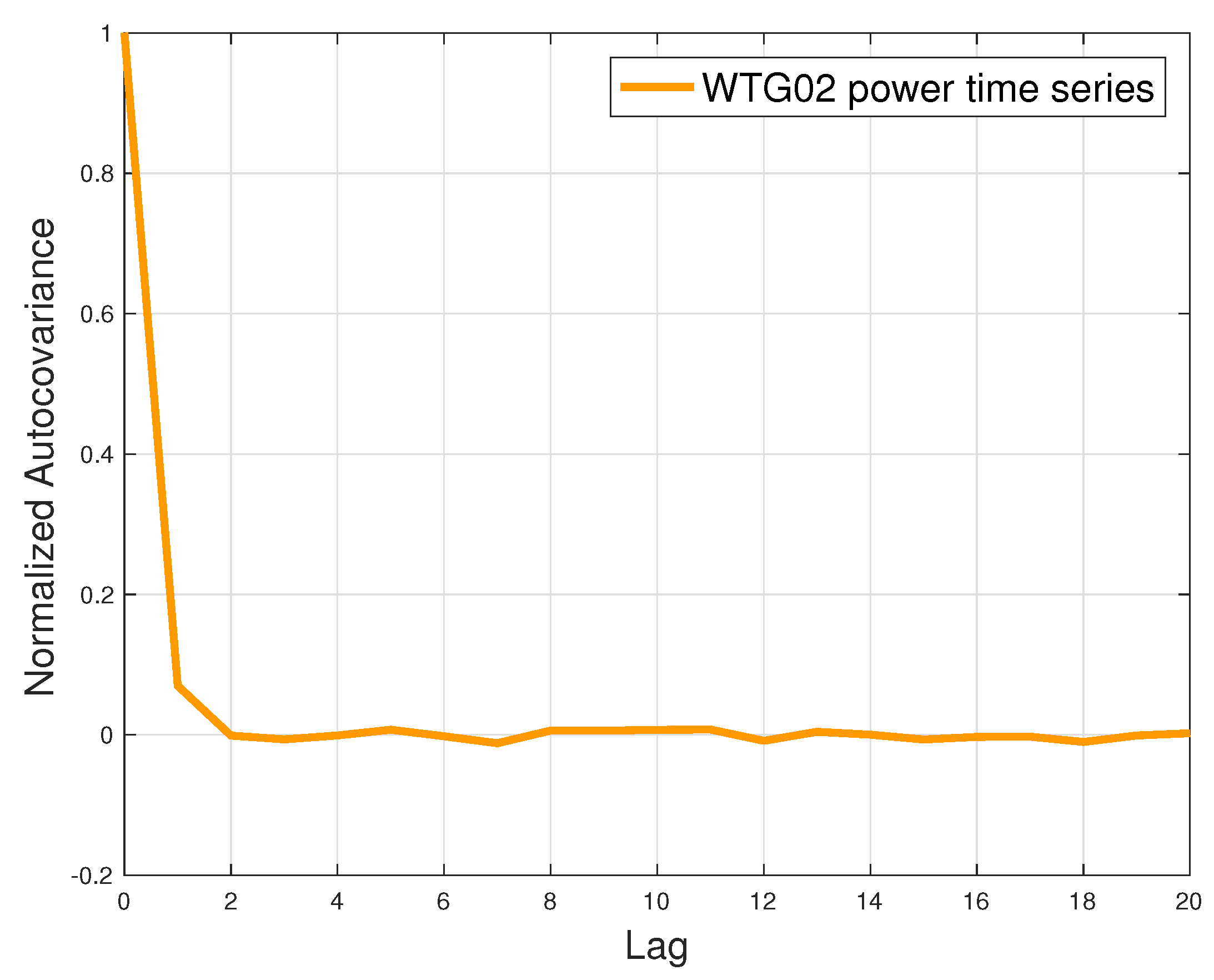
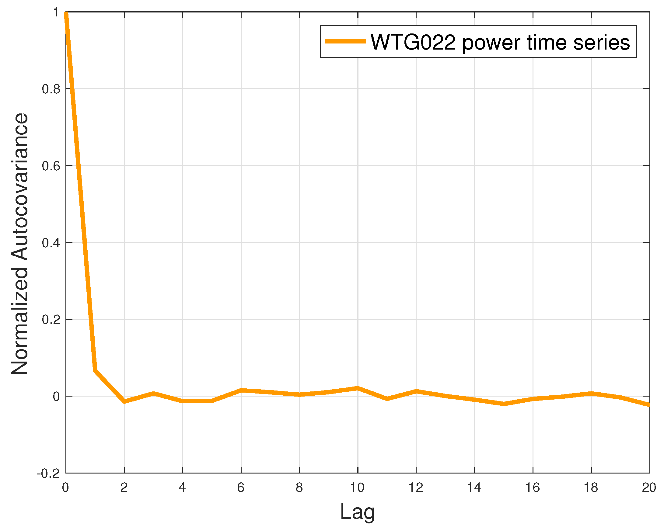
In Figure 2, the normalized autocovariance of the power output of WTG02 is reported as a function of the lag (up to 20) for the dataset. This was done to crosscheck the assumption that each measurement can be considered independent with respect to the others.
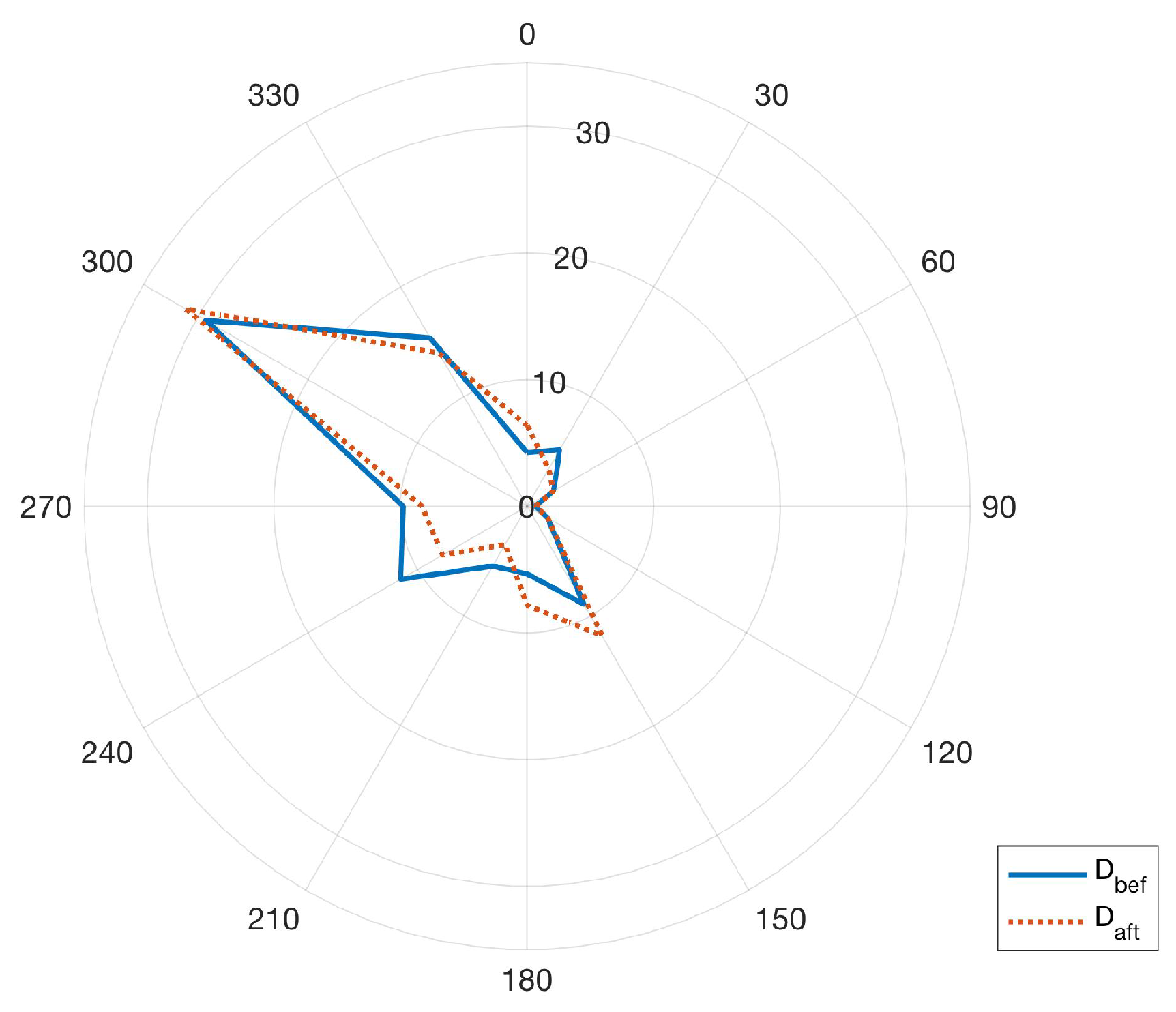
The wind direction roses, measured at WTG02, during and are reported in Figure 3 and it arises that the distributions are very similar before and after the upgrade of the WTG02. Therefore, it can be argued that, as far as can be analyzed from the data available, the model formulation and use are not biased by differences in climatology. This is supported also by the fact that the ratio between the average nacelle wind speeds at WTG02 during and is 1.04.
The SCADA collected data have ten minutes of sampling time. The available validated measurements are:
- nacelle wind speed;
- nacelle wind direction;
- nacelle position;
- temperature outside the nacelle;
- active power;
- rotor rotational speed;
- generator rotational speed; and
- reference blade pitch.
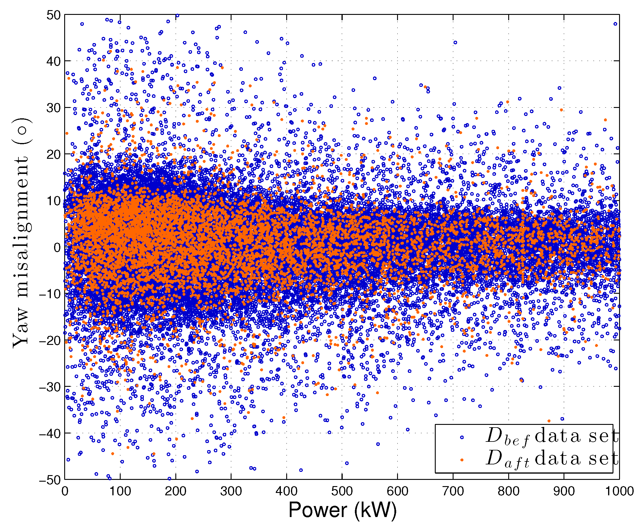
The effect of the control upgrade was an improvement of the yaw management, especially for low and moderate wind intensities. This resulted in a decrease of the occurrence of high yaw misalignment. Qualitatively, this was assessed as follows: the yaw misalignment of WTG02 was computed as the difference between the wind direction measured at the nacelle and the position of the nacelle itself. As a pre-requisite, data were filtered on the request that WTG02 was in production. The plot of the yaw misalignment (in degrees) against the power is reported in Figure 4 for the datasets and .
2.2. Test Case 2: Control Re-Powering, 850 kW Wind Turbine
The wind farm of interest is composed of twenty-three horizontal-axis three-bladed wind turbines having 850 kW of rated power each and the rotor diameter is 58 m. The cut-in is 3 m/s and the cut-out is 20 m/s. The nominal wind speed is 12.5 m/s.
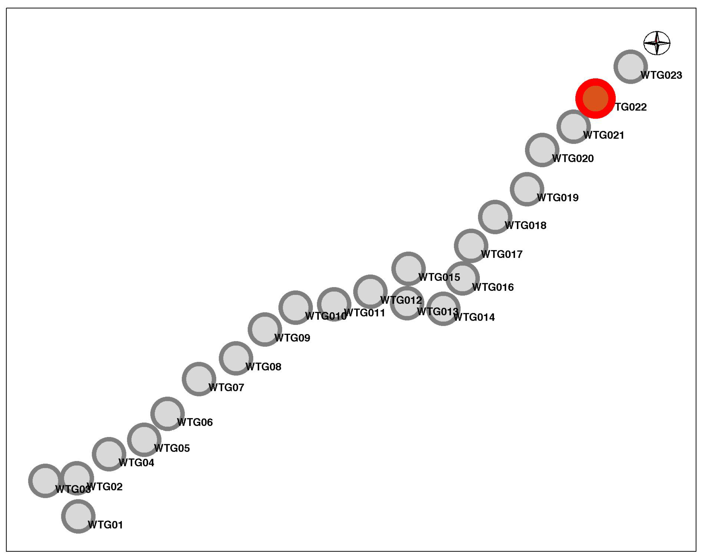
The layout of the wind farm is reported in Figure 5 and the wind turbine of interest (WTG022) is indicated in red. The wind farm is sited onshore in a gentle terrain in northern France. The inter-turbine distances go from the order of four rotor diameters (between nearest neighbors) to the order of 100 rotor diameters. The wind direction rose on-site is quite uniform.
The data available were organized into two datasets as follows:
- The first dataset is denoted as and contains the data collected from 1 February 2018 to 20 August 2018. It is a period prior to the control upgrade on turbine WTG022. It is composed of 15,353 data.
- The second dataset is denoted as and contains the data collected from 24 August 2018 to 1 April 2019. It is a period after the control optimization on turbine WTG022. In this period, half-hour intervals of operation according to the pre- and post-upgrade logic were alternated. The former subset is indicated as and is composed of 4245 data. The latter subset is indicated as and is composed of 4265 data. Only is employed for the model-based estimate of the upgrade, while both subsets are employed for the power curve study in Section 4.2.1.
In Figure 6, the normalized autocovariance of the power output of WTG022 is reported as a function of a lag up to 20, for the dataset. This was done to crosscheck the assumption that each measurement can be considered independent with respect to the others.
The wind direction roses, measured at WTG022, during and are reported in Figure 7 and it arises that the distributions are similar before and after the upgrade of the WTG022. Therefore, it can be argued that, as far as can be analyzed from the data available, the model formulation and use are not remarkably biased by climatology effects. This is supported also by the fact that the ratio between the average nacelle wind speeds at WTG02 during and is 0.96.
The SCADA collected data have ten minutes of sampling time. The available validated measurements are:
- nacelle wind speed;
- temperature outside the nacelle; and
- active power.
It should be noticed that, after the upgrade intervention, WTG022 has a sonic anemometer at the nacelle. As discussed in detail in Section 4.2.1, the operation of WTG022 during was as follows: half-hour intervals of operation according to the pre- and post-upgrade control logic were alternated. Therefore, to assess the upgrade using the techniques proposed in Section 3, only the data in characterized by operation according to the upgraded control were selected. Instead, for the power curve study of Section 4.2.1, all data in were used, after dividing them according to the pre or post upgrade behavior.
3. The Methods
This section presents the formulating of a reliable model for the pre-upgrade power of the wind turbines of interest (WTG02 in Wind Farm 1 and WTG022 in Wind Farm 2). Section 4 is devoted in detail to the use of these models for the performance improvement estimate. For the moment, it is important to recall that a good model for the power of the wind turbines was needed because it was trained with pre-upgrade data and validated against a pre-upgrade dataset; the upgrade was quantified by simulating through the adopted model how the post-upgrade power would have been if the upgrade did not take place. In other words, the performance improvement was elaborated from how the residuals between measurements and model estimates changed after the upgrade with respect to before.
As anticipated in Section 1, the critical point was selecting the model type and the input variables. The discussion in [33], in relation to the work in [25], indicates that a linear model can be adequate for this objective. In other words, the general sense is that it is possible to approximate reliably the power of a wind turbine as a linear function of operation variables measured at the nearby wind turbines in the farm. This makes sense, not only by a statistical point of view, but also by the point of view of wind energy practice: actually, since a wind turbine acts as a filter to the wind fluctuations, the blade pitch, the rotor revolutions per minute and the active power of a wind turbine can likely be used for accounting for the on-site wind conditions [36].
The possible variables fed as input to the model are those indicated in Section 2.1 for Test Case 1 and those indicated in Section 2.2 for Test Case 2, for all the wind turbines in the wind farms except the upgraded ones. The decision of excluding the variables of the upgraded wind turbines as input variables to the model was motivated by the fact that the wind sensors might change after the upgrade (as in Test Case 2, see Section 2.2), or the upgrade might affect the measuring chain of the wind conditions (as discussed in [25,33]), or in general the relation between the power and the control (pitch, rotor revolutions per minute, etc) might change as a consequence of the upgrade. Therefore, since for the employed method one must assume that the input variables to the model are “probes” of the external conditions whose behavior does not change after the upgrade of the wind turbine of interest, it is straightforward that the variables of the upgraded wind turbine can only be the target (i.e., the output) of the model.
Similar to Astolfi et al. [33], a linear model was considered adequate for the objectives of this work. The critical point is the input variables selection: Table 1 and Table 2 indicate that the possible covariates of the model can be highly correlated and this would lead to a non-optimal standard linear regression. On these grounds, Principal Component Regression (PCR) [39] was selected for this study. The use of this method for control and monitoring purposes in wind energy has been growing [40]. The procedure is as follows. Let be the vector of measured output and be the matrix of covariates. n is the number of observations and p is the number of covariates. In the following, it is assumed that is normalized such that each covariate has zero mean.
The standard least squares regression poses that
where is the vector of regression coefficients that must be estimated from the data and is a vector of random errors. The ordinary least squares estimate of is given by
The principal component estimate of is obtained as follows. The principal component transformation of the covariates matrix can easily be expressed in terms of the singular value matrix factorization. Therefore, let
be the singular value decomposition of . This means that the columns of and are orthonormal sets of vectors denoting the left and right singular vectors of and is a diagonal matrix, whose elements are the singular values of . This allows decomposing as:
where and .
is the ith principal component and is the ith loading corresponding to the ith principal value . Therefore, can be viewed as a new covariates data matrix and the principal component regression basically is an ordinary least squares regression between and . A powerful aspect of the principal component regression is that the decomposition in Equation (4) indicates a sort of regularization scheme: namely, the matrix can be truncated including a desired number of principal components. This regularization addresses the problem of multicollinearity of covariates, because, when two or more covariates are highly correlated, tends to lose its full rank and this implies that has some eigenvalues tending to 0: excluding the principal components associated to the smallest eigenvalues means regularizing the covariates matrix in order that it has full rank.
Finally, the PCR estimate of is given as
where it is assumed that the matrices can be truncated to a desired number of columns, i.e., principal components.
The selection of an adequate number of principal components for the regression is performed through K-fold cross-validation [41]. is divided randomly in two fractions: of the data are used for training and the remaining are used for validation. K was selected to be 10 for this study. The training data are employed for estimating through principal component regression (Equation (5)) and the model estimate of the validation data is given by
For each fold selection, the root mean square error is used as a metric for the goodness of the regression: it is given in general by
where is the number of rows of . The values are subsequently averaged on the folds selection and, therefore, for a given number j of principal components included in the regression, one can obtain a unique metric for estimating the quality of the regression. The final selection of the number of principal components to be kept is performed as follows: given , the error estimate for the model with j principal components, if , k is selected. It should be noticed that, as discussed in Section 4, the results for both test cases do not depend sensibly on this choice, as long as a certain minimum number of principal components are included in the model.
A test can be formulated for inquiring the statistical significance of the fact the performance of the wind turbine of interest has changed after the upgrade. One can pose that the output can be modeled through a linear model before and after the upgrade and inquire to whether there has been a structural change, i.e. if the linear models before and after the upgrade are different. Suppose therefore that
where is the matrix of explanatory variables, is the vector of regression coefficients and are vectors of random errors.
The hypothesis test about the structural change of the regression regards the null hypothesis:
This is known as the Chow test and is based on the fact that, indicated with the residuals sum of squares between measurements and model estimates, the quantity
is distributed as , where K is the number of covariates and N is the number of data points.
Practically, the Chow test is performed as follows. The covariates matrices and the output vectors before and after the upgrade are vertically juxtaposed to form a total covariates matrix and a total output vector . The test is performed with the assumption that the break point where the structural change can happen occurs when the data before the upgrade end and the data after the upgrade start.
3.1. Test Case 1
In Table 2, some sample results are reported for supporting the selection of the principal component regression: the correlation coefficients between the rotor rotational speeds of WTG01 and WTG03–WTG06 are reported. These covariates were selected because the rotor basically acts as a filter, smoothing the fluctuations caused by the turbulence, and it is therefore likely that in a wind farm the rotor speeds of nearby wind turbines are highly collinear.
The structure of the model for the test case of interest was selected as follows. The output is the power of WTG02; the covariates matrix was selected to be composed of power, rotor rotational speed, generator rotational speed, blade pitches, nacelle position and ambient temperature at each wind turbine of the wind farm, except WTG02. Therefore, if one considers the filtered dataset, is a vector of 25,044 data and is a matrix having 24,055 rows and 30 columns (six variables for five wind turbines).
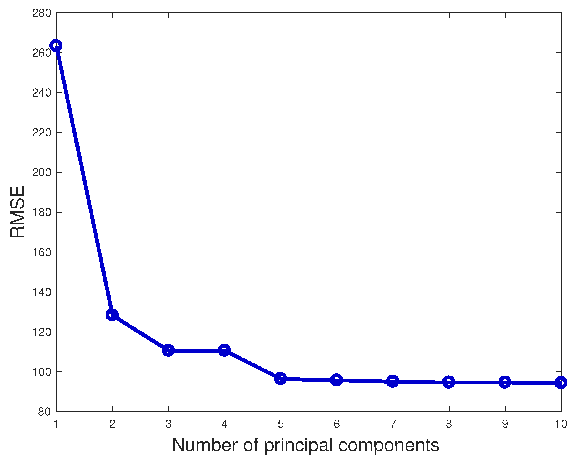
The results for the model K-fold cross-validation are reported in Figure 8 and, with the criterion exposed in Section 3, five principal components were selected. It should be noticed that a sensitivity analysis was carried and it was observed that the results do not change substantially by including more than five principal components.
As regards the Chow Test, the matrix is composed of 31,392 rows (25,044 before upgrade and 6348 after upgrade) and 30 columns, and the vector is composed of 31392 elements. The break point position for the Chow test is 25,044 and the computed p-value is lower than . This clearly indicates that the linear relation between covariates matrix and the target has a structural change after the upgrade of WTG02.
3.2. Test Case 2
In Table 2, the correlation coefficients between some sample covariates are reported. The powers of WTG018–WTG021 and WTG023 was selected for reporting in Table 2: these covariates was selected for readability of the table and mostly because those wind turbines are the nearest to the target WTG022 and therefore those covariates are likely to be selected for a standard least squares regression. The remarkably high values reported in Table 2 support the selection of the principal component regression as model type.
The structure of the model for the test case of interest was selected as follows. The output is the power of WTG022. The covariates matrix is composed of the available validated measurements: nacelle wind speed, power and ambient temperature at each wind turbine of the wind farm, except WTG022. Therefore, if one considers the filtered dataset, is a vector of 15,353 data and is a matrix having 15,353 rows and 66 columns (three variables for 22 wind turbines).
The results for the model K-fold cross-validation are reported in Figure 9 and, through the criterion exposed in Section 3, the number of selected principal components results to be six. It should be noticed that the results do not change significantly by including more than six principal components in the model.
As regards the Chow Test, the matrix is composed of 19,618 rows (15,353 before upgrade and 4265 after upgrade) and 66 columns, the vector is composed of 19,618 elements. The break point position for the Chow test is 15,353 and the computed p-value is lower than . This clearly indicates that the linear relation between covariates matrix and the target has a structural change after the upgrade of WTG022.
4. The Results
The procedure for assessing the upgrade Was based on the following idea. After an upgrade installation, through the SCADA collected data, it is possible to know the power production of the upgraded wind turbine. To estimate the impact of the upgrade, one should know how much the wind turbine would have produced if the upgrade did not take place. The most reliable and practical way to obtain this kind of estimate is through a data-driven model, based on the pre-upgrade datasets. A reliable model was achieved (Section 3) and it was used for the upgrade assessment presented below.
The procedure is as follows. The datasets available were organized in this way:
- was randomly divided in two subsets: D0 ( of the data) and D1 ( of the data). D0 was used for training the model and constructing the weight matrix and D1, the pre-upgrade dataset, was employed for validating the model.
- , the post-upgrade dataset, was employed for estimating the power upgrade. For notation consistency, it is also referred to equivalently as D2.
Notice that, for Test Case 2, the dataset was employed as D2.
The residuals between the measurement y and the simulation , for the datasets D1 and D2, were studied. The focus was in how the residuals varied after the upgrade. Therefore, consider Equation (11) with .
A Student’s t-test was performed to inquire if there was any statistically significant change in the turbine output after the upgrade. The t statistic is computed as
In Equation (12), and are the numbers of data in, respectively, D1 and D2; and are the average residuals in datasets D1 and D2 respectively; and is given in Equation (13):
where and are the standard deviations of the residuals in datasets D1 and D2, respectively.
As regards the upgrade estimate, for , one computes
and
where is the number of data points in the datasets D1 and D2, respectively. Notice that, if the model is reliable, one should have that and , differently with what should happen as regards and if the upgrade is really effective. Finally, the quantity
can be taken a percentage estimate of the production improvement. In the case the datasets D1 and D2 are characterized by considerably different y distributions, it might be appropriate to take this into account by renormalizing Equation (16): a reasonable correction factor can be the ratio between the y averages in datasets D2 and D1.
The above procedure can be repeated several times to synthesize experiment repetition: at each run of the model, a different D0 (training set) and therefore D1 (pre-upgrade validation dataset) can be selected. Notice that this basically corresponds to repeating the K-fold cross-validation. The difference with respect to the procedure described in Section 3 is that in this case the model structure was always the same and it was exactly the one selected on the grounds of the discussion in Section 3. The way the pre-upgrade data were divided was also changed with respect to Section 3. The selection of D0 and D1 actually corresponded to . This was done because it agrees with most of the rule of thumbs for data partition for this kind of tasks and because, with this selection, the dimensions of D1 and D2 (the post-upgrade dataset) have the same order of magnitude.
Therefore, the estimate varied at each run of the model, because the training data changed and, therefore and changed. In principle, it could be possible to select randomly a subset of D2 as post-upgrade simulation dataset, but in this work this choice was avoided. The reason was that typically D2 is shorter than D0 and D1, because for practical reasons an upgrade is assessed as soon as possible with good reliability. The above bootstrap technique therefore allowed having several estimates of with the same data: the final estimate was always the average and it is presented below with its standard deviation. This corresponds to the procedure of Section 3 with J repetitions: for this part of the study, J was selected based on when the average and standard deviation became fairly stable. It was observed that is sufficient for this task.
4.1. Test Case 1
Since the effect of the upgrade regards especially the low-moderate wind intensity, data were filtered on the request that the power of WTG02 is less than 1 MW. After this further filter, the number of data was 25,044 for and 6348 for .
The t-statistic (Equation (12)) was computed to be of the order of and this indicates that the probability that the upgrade was ineffective was correspondingly low.
Table 3 reports the results for the average (over the J model runs) and with (Equations (14) and (15)). From these results, it arises that the upgrade could be detected as an average absolute increase of 13.5 kW in the difference between WTG02 power measurements and model estimates. Notice that the average value of the residuals for datasets D1 was extremely low (0.1 kW) and, correspondingly, the average estimate of (Equation (16)), i.e. the percentage error on the cumulative production, was extremely low as well. This indicates that the model was particularly reliable as regards the simulation of the pre-upgrade behavior of the WTG02.
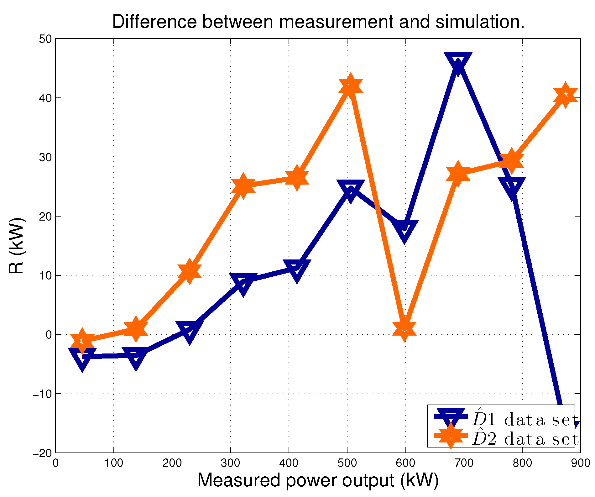
In Figure 10, the plot of and on a sample model run is reported. The data were averaged in power production intervals, whose amplitude was 5% of the rated. From this plot, the effect of the upgrade can be read as an increase of the difference between the WTG02 power measurements and the WTG02 power model estimates.
From the results in Table 3 and Equation (14), the average production improvement was estimated as , with a standard deviation of 0.4%: in other words, with the proposed method it was computed that WTG02, during the dataset D2, produced below 1 MW, the 4.1% more than it would have done if the upgrade had not been adopted. A reference long-term power or wind speed distribution can be employed to estimate how much this corresponds in terms of annual energy production and the average result is . This result is consistent with the test case studies in [25]: the order of magnitude of the impact of multi-megawatt wind turbine control optimization can typically be estimated as 1% of the AEP. It is interesting notice that, to the best of the authors knowledge, this is the first estimate in the literature based on operation data of the impact of yaw control optimization.
4.2. Test Case 2
The t-statistic (Equation (12)) was computed to be of the order of and this indicates that the probability that the upgrade was ineffective was correspondingly low.
Table 4 reports the results for the average (over the J model runs) and with (Equations (14) and (15)). It arises that the upgrade could be detected as an average absolute increase of 3.9 kW in the difference between WTG022 power measurements and model estimates. The average value of the residuals for datasets D1 was very low (0.2 kW) and correspondingly, the average estimate of (Equation (16)), i.e. the percentage error on the cumulative production, was extremely low as well. This indicates that the model was reliable as regards the simulation of the pre-upgrade behavior of the WTG022.
In Figure 11, the plot of and on a sample model run is reported. The data were averaged in power production intervals, whose amplitude was 10% of the rated. From this plot, the effect of the upgrade can be read as an increase of the difference between the WTG022 power measurements and the WTG022 power model estimates, especially for moderately low wind intensities and approaching rated power.
From the results in Table 3 and Equation (14), the average production improvement was estimated as , with a standard deviation of 0.2%: in other words, with the proposed method it was computed that WTG022, during the dataset D2, produced 2.5% more than it would have done if the upgrade had not been adopted.
Power Curve Analysis
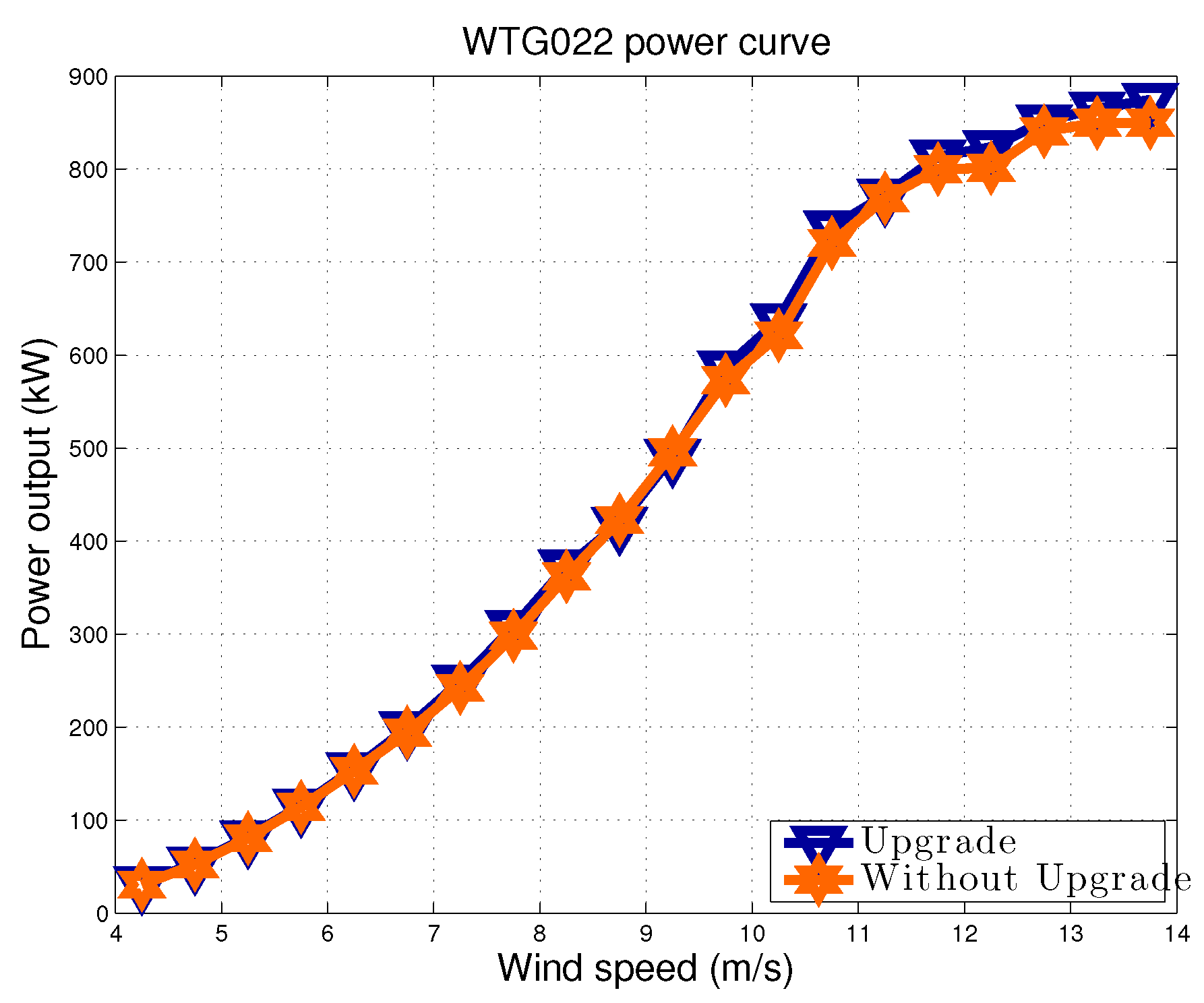
As anticipated in Section 2, the post-upgrade operation during dataset was as follows: half-hour intervals were alternated, during which WTG022 was operating, respectively, according to the pre- and post-upgrade control logic. This was done to assess practically in real time the effect of the upgrade. With these data available and taking into account that, during , a sonic anemometer was collecting data at WTG022 nacelle, it was reasonable to study the power curve.
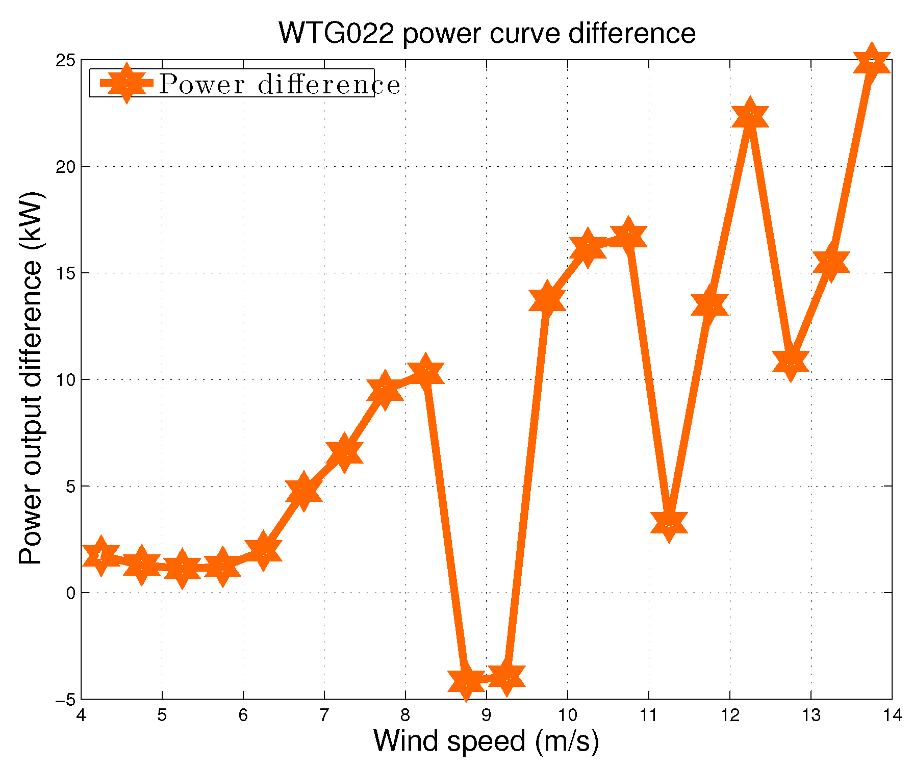
In Figure 12, the two power curves measured during are reported. Data were averaged in wind speed intervals having 0.5 m/s of amplitude. In Figure 13, the difference between these two curves is plotted. In Figure 13, it can interestingly be observed that the upgraded operation mode indeed lost performance around 10 m/s: the same situation was observed from the residuals presented in Figure 11. Since this study was performed with only few months of data in , it is plausible to expect that this situation was adjusted in the following, to obtain a performance improvement along the whole power curve.
The production improvement was estimated as follows: the power curve, according to the pre-upgrade logic in Figure 12, and the power difference in Figure 13, were weighted against the wind distribution during the whole dataset. The ratio between these two quantities provided an estimate of how much the production would have improved during if the power curve was always the improved one, with respect to the production that would have been obtained if the power curve was always the non-improved one. The improvement computed in this way amounted to 2.3% of the production. Even though it was computed with a different approach, it is interesting to notice that it agreed fairly well with the estimate reported in Section 4.2.
5. Conclusions
In this study, two test cases of wind turbine power curve upgrades were analyzed: the common ground between them is that the upgrade regards the control of the wind turbines. The difference between the two test cases is that one wind turbine (Test Case 1) has a quite recent technology (it is a 2 MW wind turbine) and the control upgrade deals only with one aspect (the management of the yaw); the other wind turbine under investigation (Test Case 2) belongs instead to a less recent technology (the rated power is 850 kW) and the upgrade has consequently involved several aspects of the control (yaw, pitch, and cut-out) and included the update of the anemometer sensors at the nacelle.
Despite being organized as a test case discussion, this study was strongly characterized by a methodological approach. Actually, the point with the study of wind turbine power curve upgrades is that it is difficult to assess them reliably using operation data analysis techniques such as the power curve, because of the multivariate dependence of the power of a wind turbine on climate conditions and working parameters. The problem of wind turbine power curve upgrades study therefore translates into the following question: how can the power of a wind turbine be modeled reliably? It is evident that the answer to this question can be exploited for several problems regarding the control and monitoring of wind turbines and, in general, of complex systems. As regards wind turbines, for example, similar approaches are employed in [42] for the study of how much the pitch misalignment impacts on the performance.
The turning point for the present study was practically adopting the other wind turbines in the wind farm as probes of on-site conditions. This somehow generalized the concept of rotor-equivalent wind speed, discussed, for example, in [36]: since the wind turbine acts as a filter, some working parameters such as active power, blade pitches, rotor or generator revolutions per minute can robustly describe the wind farm at the micro-scale level. Therefore, the idea of this study was modeling the power of the wind turbines of interest, according to their pre-upgrade behavior, as a linear function of the wind and operation conditions measured at the nearby wind turbines: this can basically be considered a generalization of the so-called power–power method, adopted, for example, in [30]. Since for the test cases considered in this work the possible covariates for a linear model displayed a remarkable collinearity, a principal component regression was adopted.
Using this modeling technique, the impact of the upgrades could be elaborated from how the residuals between power measurements and power model estimates vary after the upgrade with respect to before. The results for the selected test cases are the following: the yaw control optimization on the 2 MW wind turbine was estimated as 1.3% of the AEP; and the re-powering on the 850 kW wind turbine was estimated as 2.5% of the AEP.
There are at least two other remarkable aspects as regards the selected test cases. To the best of the authors knowledge, Test Case 1 is the first assessment in the literature of yaw control optimization using operation data and the obtained results indicate that the yaw management optimization is a promising direction for improving the power production of wind turbines. It is therefore valuable to push forward this line of research, as recently done, for example, in [35]. As regards Test Case 2, it was possible to obtain another estimate of the impact of the upgrade using the power curve study. Actually, with the re-powering, the anemometer sensors were updated and a sonic anemometer was installed. Furthermore, in the post upgrade period examined for this study, the operation of the wind turbine was alternated: half an hour according to the pre-upgrade logic and half an hour according to the post-upgrade logic, and so on. The quality of the data and the fact that they were collected in the same period (avoiding seasonal biases) allowed studying the power curve reliably and the improvement estimate was shown to be in good agreement with the computation from the multivariate model.
There are several further directions of the present work. Currently, some test cases are at study for which a linear model is not adequate, probably because of complex climatology conditions on site. Therefore, it is planned to investigate nonlinear approaches for this kind of studies and to inquire what site characteristics call for nonlinearity. An interesting development is the use of the methods of this work for other control and monitoring issues related to wind turbine operation: for example, monitoring the effect of blade pitches re-alignment according to the technique proposed in [43], or monitoring the operation of the wind turbines [40]. Furthermore, a very promising direction of the studies about wind turbine power curve upgrades is the use of time-resolved data, having sampling time of the order of second: this kind of data have considerable potentiality for performance control and monitoring [44], but their time scale calls for more advanced time-series analysis [45].
Author Contributions
Conceptualization, D.A. and F.C.; Data curation, D.A.; Formal analysis, D.A.; Investigation, D.A., F.C.; Methodology, D.A.; Project administration, F.C.; Software, D.A.; Supervision, F.C., Validation, D.A.; Writing—original draft, D.A.; and Writing— review adn editing, F.C.
Funding
This research received no external funding.
Acknowledgments
The authors thank Ludovico Terzi, technology manager of Renvico.
Conflicts of Interest
The authors declare no conflict of interest.
References
- Tchakoua, P.; Wamkeue, R.; Ouhrouche, M.; Slaoui-Hasnaoui, F.; Tameghe, T.A.; Ekemb, G. Wind turbine condition monitoring: State-of-the-art review, new trends, and future challenges. Energies 2014, 7, 2595–2630. [Google Scholar] [CrossRef]
- Parada, L.; Herrera, C.; Flores, P.; Parada, V. Wind farm layout optimization using a Gaussian-based wake model. Renew. Energy 2017, 107, 531–541. [Google Scholar] [CrossRef]
- Shakoor, R.; Hassan, M.Y.; Raheem, A.; Wu, Y.K. Wake effect modeling: A review of wind farm layout optimization using Jensen’s model. Renew. Sustain. Energy Rev. 2016, 58, 1048–1059. [Google Scholar] [CrossRef]
- Feng, J.; Shen, W.Z. Solving the wind farm layout optimization problem using random search algorithm. Renew. Energy 2015, 78, 182–192. [Google Scholar] [CrossRef]
- Sorkhabi, S.Y.D.; Romero, D.A.; Yan, G.K.; Gu, M.D.; Moran, J.; Morgenroth, M.; Amon, C.H. The impact of land use constraints in multi-objective energy-noise wind farm layout optimization. Renew. Energy 2016, 85, 359–370. [Google Scholar] [CrossRef]
- Chen, Y.; Li, H.; He, B.; Wang, P.; Jin, K. Multi-objective genetic algorithm based innovative wind farm layout optimization method. Energy Convers. Manag. 2015, 105, 1318–1327. [Google Scholar] [CrossRef]
- Park, J.; Law, K.H. Cooperative wind turbine control for maximizing wind farm power using sequential convex programming. Energy Convers. Manag. 2015, 101, 295–316. [Google Scholar] [CrossRef]
- Park, J.; Law, K.H. A data-driven, cooperative wind farm control to maximize the total power production. Appl. Energy 2016, 165, 151–165. [Google Scholar] [CrossRef]
- Wang, F.; Garcia-Sanz, M. Wind farm cooperative control for optimal power generation. Wind Eng. 2018, 42, 547–560. [Google Scholar] [CrossRef]
- Gebraad, P.; Thomas, J.J.; Ning, A.; Fleming, P.; Dykes, K. Maximization of the annual energy production of wind power plants by optimization of layout and yaw-based wake control. Wind Energy 2017, 20, 97–107. [Google Scholar] [CrossRef]
- Gebraad, P.; Teeuwisse, F.; Van Wingerden, J.; Fleming, P.A.; Ruben, S.; Marden, J.; Pao, L. Wind plant power optimization through yaw control using a parametric model for wake effects—A CFD simulation study. Wind Energy 2016, 19, 95–114. [Google Scholar] [CrossRef]
- Fleming, P.A.; Ning, A.; Gebraad, P.M.; Dykes, K. Wind plant system engineering through optimization of layout and yaw control. Wind Energy 2016, 19, 329–344. [Google Scholar] [CrossRef]
- Campagnolo, F.; Petrović, V.; Bottasso, C.L.; Croce, A. Wind tunnel testing of wake control strategies. In Proceedings of the IEEE American Control Conference (ACC), Boston, MA, USA, 6–8 July 2016; pp. 513–518. [Google Scholar]
- Fleming, P.; Annoni, J.; Shah, J.J.; Wang, L.; Ananthan, S.; Zhang, Z.; Hutchings, K.; Wang, P.; Chen, W.; Chen, L. Field test of wake steering at an offshore wind farm. Wind Energy Sci. 2017, 2, 229–239. [Google Scholar] [CrossRef] [Green Version]
- Barlas, T.K.; Van Kuik, G. Review of state of the art in smart rotor control research for wind turbines. Prog. Aerosp. Sci. 2010, 46, 1–27. [Google Scholar] [CrossRef]
- Tsai, K.C.; Pan, C.T.; Cooperman, A.M.; Johnson, S.J.; Van Dam, C. An innovative design of a microtab deployment mechanism for active aerodynamic load control. Energies 2015, 8, 5885–5897. [Google Scholar] [CrossRef]
- Fernández-Gámiz, U.; Marika Velte, C.; Réthoré, P.E.; Sørensen, N.N.; Egusquiza, E. Testing of self-similarity and helical symmetry in vortex generator flow simulations. Wind Energy 2016, 19, 1043–1052. [Google Scholar] [CrossRef]
- Aramendia, I.; Fernandez-Gamiz, U.; Ramos-Hernanz, J.A.; Sancho, J.; Lopez-Guede, J.M.; Zulueta, E. Flow Control Devices for Wind Turbines. In Energy Harvesting and Energy Efficiency; Springer: Berlin, Germany, 2017; pp. 629–655. [Google Scholar]
- Fernandez-Gamiz, U.; Zulueta, E.; Boyano, A.; Ansoategui, I.; Uriarte, I. Five megawatt wind turbine power output improvements by passive flow control devices. Energies 2017, 10, 742. [Google Scholar] [CrossRef]
- Fernandez-Gamiz, U.; Gomez-Mármol, M.; Chacón-Rebollo, T. Computational Modeling of Gurney Flaps and Microtabs by POD Method. Energies 2018, 11, 2091. [Google Scholar] [CrossRef]
- Gutierrez-Amo, R.; Fernandez-Gamiz, U.; Errasti, I.; Zulueta, E. Computational Modelling of Three Different Sub-Boundary Layer Vortex Generators on a Flat Plate. Energies 2018, 11, 3107. [Google Scholar] [CrossRef]
- Fernandez-Gamiz, U.; Errasti, I.; Gutierrez-Amo, R.; Boyano, A.; Barambones, O. Computational Modelling of Rectangular Sub-Boundary Layer Vortex Generators. Appl. Sci. 2018, 8, 138. [Google Scholar] [CrossRef]
- Aramendia, I.; Fernandez-Gamiz, U.; Zulueta, E.; Saenz-Aguirre, A.; Teso-Fz-Betoño, D. Parametric Study of a Gurney Flap Implementation in a DU91W (2) 250 Airfoil. Energies 2019, 12, 294. [Google Scholar] [CrossRef]
- Lee, G.; Ding, Y.; Xie, L.; Genton, M.G. A kernel plus method for quantifying wind turbine performance upgrades. Wind Energy 2015, 18, 1207–1219. [Google Scholar] [CrossRef]
- Astolfi, D.; Castellani, F.; Terzi, L. Wind Turbine Power Curve Upgrades. Energies 2018, 11, 1300. [Google Scholar] [CrossRef]
- Astolfi, D.; Castellani, F.; Berno, F.; Terzi, L. Numerical and Experimental Methods for the Assessment of Wind Turbine Control Upgrades. Appl. Sci. 2018, 8, 2639. [Google Scholar] [CrossRef]
- Bossanyi, E.; King, J. Improving wind farm output predictability by means of a soft cut-out strategy. In Proceedings of the European Wind Energy Conference and Exhibition EWEA, Copenhagen, Denmark, 16–19 April 2012; Volume 2012. [Google Scholar]
- Petrović, V.; Bottasso, C.L. Wind turbine optimal control during storms. J. Phys. Conf. Ser.. 2014, 524, 012052. [Google Scholar] [CrossRef] [Green Version]
- Astolfi, D.; Castellani, F.; Lombardi, A.; Terzi, L. About the extension of wind turbine power curve in the high wind region. J. Solar Energy Eng. 2019, 141, 014501. [Google Scholar] [CrossRef]
- Hwangbo, H.; Ding, Y.; Eisele, O.; Weinzierl, G.; Lang, U.; Pechlivanoglou, G. Quantifying the effect of vortex generator installation on wind power production: An academia-industry case study. Renew. Energy 2017, 113, 1589–1597. [Google Scholar] [CrossRef]
- Astolfi, D.; Castellani, F.; Terzi, L. A SCADA data mining method for precision assessment of performance enhancement from aerodynamic optimization of wind turbine blades. J. Phys. Conf. Ser. 2018, 1037, 032001. [Google Scholar] [CrossRef]
- Terzi, L.; Lombardi, A.; Castellani, F.; Astolfi, D. Innovative methods for wind turbine power curve upgrade assessment. J. Phys. Conf. Ser. 2018, 1102, 012036. [Google Scholar] [CrossRef]
- Astolfi, D.; Castellani, F.; Fravolini, M.L.; Cascianelli, S.; Terzi, L. Precision Computation of Wind Turbine Power Upgrades: An Aerodynamic and Control Optimization Test Case. J. Energy Resour. Technol. 2019, 141, 051205. [Google Scholar] [CrossRef]
- Song, D.; Yang, J.; Fan, X.; Liu, Y.; Liu, A.; Chen, G.; Joo, Y.H. Maximum power extraction for wind turbines through a novel yaw control solution using predicted wind directions. Energy Convers. Manag. 2018, 157, 587–599. [Google Scholar] [CrossRef]
- Saenz-Aguirre, A.; Zulueta, E.; Fernandez-Gamiz, U.; Lozano, J.; Lopez-Guede, J.M. Artificial Neural Network Based Reinforcement Learning for Wind Turbine Yaw Control. Energies 2019, 12, 436. [Google Scholar] [CrossRef]
- Wagner, R.; Cañadillas, B.; Clifton, A.; Feeney, S.; Nygaard, N.; Poodt, M.; St Martin, C.; Tüxen, E.; Wagenaar, J. Rotor equivalent wind speed for power curve measurement—Comparative exercise for IEA Wind Annex 32. J. Phys. Conf. Ser. 2014, 524, 012108. [Google Scholar] [CrossRef]
- Green, W.H. Econometric Analysis; Maxwell Macmillan International: New York City, NY, USA, 1997. [Google Scholar]
- Pope, P.; Webster, J. The use of an F-statistic in stepwise regression procedures. Technometrics 1972, 14, 327–340. [Google Scholar] [CrossRef]
- Frank, L.E.; Friedman, J.H. A statistical view of some chemometrics regression tools. Technometrics 1993, 35, 109–135. [Google Scholar] [CrossRef]
- Pozo, F.; Vidal, Y. Wind turbine fault detection through principal component analysis and statistical hypothesis testing. Energies 2016, 9, 3. [Google Scholar] [CrossRef]
- Refaeilzadeh, P.; Tang, L.; Liu, H. Cross-validation. In Encyclopedia of Database Systems; Springer: Berlin, Germany, 2009; pp. 532–538. [Google Scholar]
- Astolfi, D. A Study of the Impact of Pitch Misalignment on Wind Turbine Performance. Machines 2019, 7, 8. [Google Scholar] [CrossRef]
- Elosegui, U.; Egana, I.; Ulazia, A.; Ibarra-Berastegi, G. Pitch angle misalignment correction based on benchmarking and laser scanner measurement in wind farms. Energies 2018, 11, 3357. [Google Scholar] [CrossRef]
- Gonzalez, E.; Stephen, B.; Infield, D.; Melero, J.J. Using high-frequency SCADA data for wind turbine performance monitoring: A sensitivity study. Renew. Energy 2019, 131, 841–853. [Google Scholar] [CrossRef]
- Rodrigues, P.M.; Salish, N. Modeling and forecasting interval time series with threshold models. Adv. Data Anal. Classif. 2015, 9, 41–57. [Google Scholar] [CrossRef]
Figure 1.
The layout of Wind Farm 1.

Figure 2.
The normalized autocovariance of WTG02 power output ( dataset) with maximum lag of 20.

Figure 3.
The wind direction rose for Wind Farm 1 during and .

Figure 4.
WTG02 yaw angle misalignment as a function of the power, for datasets and .

Figure 5.
The layout of Wind Farm 2.

Figure 6.
The normalized autocovariance of WTG022 power output ( dataset) with maximum lag of 20.

Figure 7.
The wind direction rose for Wind Farm 1 during and .

Figure 8.
Average as a function of the number of principal components included in the regression.

Figure 9.
Average as a function of the number of principal components included in the regression.

Figure 10.
The average difference R between power measurement y and estimation (Equation (11)). Datasets: D1 and D2. Sample run of the model.
Figure 10.
The average difference R between power measurement y and estimation (Equation (11)). Datasets: D1 and D2. Sample run of the model.

Figure 11.
The average difference R between power measurement y and estimation (Equation (11)). Datasets: D1 and D2. Sample run of the model.
Figure 11.
The average difference R between power measurement y and estimation (Equation (11)). Datasets: D1 and D2. Sample run of the model.

Figure 12.
WTG022 power curve during .

Figure 13.
Difference between the WTG022 power curves of Figure 12.
Figure 13.
Difference between the WTG022 power curves of Figure 12.


Table 1.
Matrix of model input variables correlation coefficients.
| WTG | 01 | 03 | 04 | 05 | 06 |
|---|---|---|---|---|---|
| 01 | 1 | 0.82 | 0.90 | 0.89 | 0.79 |
| 03 | 0.82 | 1 | 0.86 | 0.80 | 0.94 |
| 04 | 0.90 | 0.86 | 1 | 0.91 | 0.85 |
| 05 | 0.89 | 0.80 | 0.91 | 1 | 0.80 |
| 06 | 0.79 | 0.94 | 0.85 | 0.80 | 1 |
Table 2.
Matrix of model input variables correlation coefficients.
| WTG | 018 | 019 | 020 | 021 | 023 |
|---|---|---|---|---|---|
| 018 | 1 | 0.94 | 0.93 | 0.92 | 0.87 |
| 019 | 0.94 | 1 | 0.93 | 0.93 | 0.90 |
| 020 | 0.93 | 0.93 | 1 | 0.95 | 0.90 |
| 021 | 0.92 | 0.93 | 0.95 | 1 | 0.93 |
| 023 | 0.97 | 0.90 | 0.90 | 0.93 | 1 |
Table 3.
Average absolute and percentage residuals between measurement and model estimation.
| Residual | (kW) | (%) |
|---|---|---|
| 0.1 | 0.009 | |
| 13.5 | 4.1 |
Table 4.
Average absolute and percentage residuals between measurement and model estimation.
| Residual | (kW) | (%) |
|---|---|---|
| 0.2 | 0.009 | |
| 3.9 | 2.5 |
© 2019 by the authors. Licensee MDPI, Basel, Switzerland. This article is an open access article distributed under the terms and conditions of the Creative Commons Attribution (CC BY) license (http://creativecommons.org/licenses/by/4.0/).
Share and Cite
MDPI and ACS Style
Astolfi, D.; Castellani, F. Wind Turbine Power Curve Upgrades: Part II. Energies 2019, 12, 1503. https://doi.org/10.3390/en12081503
AMA Style
Astolfi D, Castellani F. Wind Turbine Power Curve Upgrades: Part II. Energies. 2019; 12(8):1503. https://doi.org/10.3390/en12081503
Chicago/Turabian StyleAstolfi, Davide, and Francesco Castellani. 2019. "Wind Turbine Power Curve Upgrades: Part II" Energies 12, no. 8: 1503. https://doi.org/10.3390/en12081503
Note that from the first issue of 2016, this journal uses article numbers instead of page numbers. See further details here.