Short-Term Load Dispatching Method for a Diversion Hydropower Plant with Multiple Turbines in One Tunnel Using a Two-Stage Model


1
Institute of Hydropower System & Hydroinformatics, Dalian University of Technology, Dalian 116024, China
2
Key Laboratory of Ocean Energy Utilization and Energy Conservation of Ministry of Education, Dalian University of Technology, Dalian 116024, China
*
Author to whom correspondence should be addressed.
Energies 2019, 12(8), 1476; https://doi.org/10.3390/en12081476
Submission received: 13 March 2019
/
Revised: 13 April 2019
/
Accepted: 15 April 2019
/
Published: 18 April 2019
(This article belongs to the Special Issue Electric Power Systems Research 2019)
Abstract
:Short-term load dispatching (STLD) for a hydropower plant with multiple turbines in one tunnel (HPMTT) refers to determining when to startup or shutdown the units of different tunnels and scheduling the online units of each tunnel to obtain optimal load dispatch while simultaneously meeting the hydraulic and electric system constraints. Modeling and solving the STLD for a HPMTT is extremely difficult due to mutual interference between units and complications of the hydraulic head calculation. Considering the complexity of the hydraulic connections between multiple power units in one tunnel, a two-phase decomposition approach for subproblems of unit-commit (UC) and optimal load dispatch (OLD) is described and a two-stage model (TSM) is adopted in this paper. In the first stage, an on/off model for the units considering duration constraints is established, and the on/off status of the units and tunnels is determined using a heuristic searching method and a progressive optimal algorithm. In the second stage, a load distribution model is established and solved using dynamic programming for optimal load distribution under the premise of the on/off status of the tunnel and units in the first stage. The proposed method is verified using the load distribution problem for the Tianshengqiao-II reservoir (TSQII) in dry season under different typical load rates. The results meet the practical operation requirements and demonstrate the practicability of the proposed method.
1. Introduction
With abundant hydropower resources, China has a total theoretical hydropower potential of 694 GW and a total technical exploitable hydropower installed capacity of 542 GW [1]. However, the spatial distribution of hydropower generation and load demands are geographically uneven in China; hydropower generation is abundant in southwestern China, while most of the energy is required in the central and southeastern areas of China. Therefore, a group of large hydro-power projects have been developed and are in development in the southwestern regions of China during the past two decades [2]. The mainstream of the Yalong River is 1571 km before joining the Yangtze River and has a service area of 136,000 km2. The river has a theoretical hydropower reserve of 33.71 GW with 99.2% of the hydropower reserve concentrated in the Sichuan Province, southwestern China. This reserve is equal to an annual power generation of 151.636 TWh, accounting for approximately 24% of the total generation of Sichuan Province. The mainstream has a natural drop of 3830 m, and a development scheme of 21 cascade reservoirs has been planned along the mainstream, which have a total capacity of 30 GW and place the river in third place among China’s 13 major hydropower bases in terms of installed capacity [3]. Simultaneously, a series of hydropower plants with multiple turbines in one tunnel [4] have been developed and are in development in southwestern China due to the influence of the geological environment, exploits, and economic conditions. Hydropower plant with multiple turbines in one tunnel (HPMTT) can be interpreted as multi-hydroturbine sets sharing a common penstock [5]. A hydropower plant with multiple turbines in one tunnel (HPMTT) with a long diversion system is illustrated in Figure 1 The Jinping-II, with the largest installed capacity in the midstream of the Yalong River, has the largest and longest hydraulic tunnels in the world and is a common example of a HPMTT. Eight Francis turbine generator sets, each with a unit capacity of 600 MW, were installed and the four headrace tunnels have a total installed capacity of 4800 MW. The Tianshengqiao-II reservoir (TSQII) is a huge hydropower station in the Hongshui River, and includes six large-size units with a total capacity of 1320 MW in the three tunnels. The Lubuge hydropower plant is the “window” of hydropower construction opening to the outside world in China and includes three hydroturbine sets sharing a common penstock. Table 1 lists the characteristics of the three hydropowerplants.
There are difficult challenges associated with the optimal operation of these hydropower plants with multiple turbines in one tunnel. The system, short-term load dispatching (STLD) for HPMTT, aims to obtain optimal load dispatch [6] and startup/shutdown costs of the units [7], but involves the grid demands, the complexity of hydraulic connections, and other electrical constraints. For instance, there are more complicated problems associated with a hydropower plant with “a hydroturbine set with a penstock” than merely a very large installed capacity, high water head, and complex vibration zones. First, changing the power generation of a unit at one period has a direct effect on the other units that share a common penstock because of the interconnected hydraulic and electrical links. The load fluctuates frequently, which makes it easier to cause water-hammer impact, and the water hammer can have potential adverse physical impacts on the performance of hydraulic installations and may impact safe operations for users and operators [8]. Furthermore, these stations are often required to respond promptly to valley loads and peak loads to maintain electric power system security and reliability. Finally, the vibration zones, combined with complex constraints such as satisfying limitations on the duration of online/offline, make it more difficult to find reasonable and feasible operations of STLD for the HPMTT. These problems present a tremendous challenge for modeling and solving an HPMTT in China. In recent years, many researchers have used various mathematical programming and optimization techniques and have considered different kinds of constraints or multiple objectives, to solve STLD problems, featuring nonlinear, nonconvex, and large-scale characteristics. These methods can be roughly divided into two categories, the stochastic optimization methods and deterministic optimization methods [9]. The stochastic optimization methods include genetic algorithm (GA) [10], ant colony optimization (ACO) [11,12], bee colony algorithm (BCA) [13], and particle swarm optimization (PSO) [2,14,15]. The above methods have achieved many achievements in the optimization of STLD problem, but there are still some shortcomings including easily falling into a local optimum and premature maturity. Moreover, the quality of the solution is susceptible to related control parameters, and selecting the control parameters for modern evolutionary algorithms is a very difficult task. The deterministic optimization methods include mixed integer linear programming (MILP) [10,16,17,18,19], dynamic programming (DP) [2,20], and improved dynamic programming methods. However, these methods each have their own disadvantages in terms of solving the STLD problem. MILP will need a large memory and cause a high computation cost with the problem size [13]. As a classic and sophisticated optimization method, the DP algorithm is still a better choice for the small scale of STLD problems due to its simple program implementation, stable computational process, and ability to search for a globally optimal solution or suboptimal solution.
Considering the disadvantages of single traditional mathematical methods and heuristic stochastic methods, hybrid algorithms [21,22] that consist of two or more methods are proposed to enhance the searching performance and accelerate the convergence process for global optimum. Compared with a single algorithm, hybrid algorithms use the advantages of each algorithm to obtain a better optimal solution [13]. As will be shown, the STLD for HPMTT is modeled by means of a mixed 0-1 Nonlinear Programming (NP) problem, and, to solve it efficiently, a two-phase decomposition approach is proposed [23]. A hybrid algorithm for solving the STLD for HPMTT problems that combines a heuristic searching method and a progressive optimal algorithm is proposed in this paper. First, the heuristic searching method and progressive optimal algorithm (POA) used to search the desirable subproblems of unit-commit (UC) for the STLD of the HPMTT problem with complicated duration period requirements are proposed. Second, more subproblems of optimal load dispatch (OLD) results are produced using the DP. Although this two-phase decomposition approach is not new, the method applied in this paper is similar to Reference [24].
This paper is organized as follows: Section 2 analyzes the influencing factors and provides the mathematical model of the STLD problem. Section 3 proposes the model solution used to solve the STLD problem. Section 4 provides the simulation results from a case study based on TSQ II. Finally, conclusions are given in Section 5.
2. Two-Stage Model
STLD for HPMTT aims to determine the on/off status of units and tunnels and the OLD results, while meeting the reservoir, tunnel, and unit constraints for one day or load demands for one week. In this paper, the dispatch horizon T is set equal to 1 day with 96 intervals. In addition to the large installed capacity, high water head, and complex vibration zones, the difficulties with the HPMTT are the various hydraulic and electric connections of different units in one tunnel. To solve these problems, a two-stage model (TSM), a unit on/off model, and a load distribution model are proposed to solve the subproblems of UC and OLD. The unit on/off model is able to coordinate different governing systems and satisfy various mutual hydraulic and electric requirements. The objective of the load distribution model is to obtain OLD while satisfying the load demands and various constraints during a given period. The TSM is connected by the on/off status of the units and the water consumption of startup/shutdown.
2.1. Influencing Factors of STLD for the HPMTT Problem
For an HPMTT, the variability of the electrical load is one of the most important factors affecting the stability of a hydroturbine governing system during operation [25,26]. Moreover, the mutual interference between units and complication of the hydraulic head calculation cannot be ignored. The principal objective of STLD for the HPMTT problem is to maximize hydropower operating efficiency and minimize total release water. Therefore, it is necessary to analyze the influencing factors of STLD for the HPMTT problem.
2.1.1. Hydraulic and Electrical Connections of HPMTT
When the load demands undergo very large fluctuations, the dynamic characteristics of the HPMTT referring to change of water level, power release, and power output are very complex, which mainly including hydraulic [9,27,28] and electrical [29] connection. The complexity of hydraulic connections is manifested by the shared hydraulic head of multiple turbines in one tunnel. When the steady state operation of one hydroturbine is disturbed, the consequent hydraulic connection affects the operation of other parallel hydroturbines installed due to the inseparable head connection of multiple power units in one tunnel. Furthermore, the complexity of electrical connections is characterized by the power balance and complex vibration zones. Meanwhile, load demand changes for a HPMTT are a key source of system instability and pose operational difficulties associated with hydraulic transient processes such as the emergency startup/shutdown of units [4]. During the emergency startup/shutdown of turbines in generating mode, the operation may frequently startup or shutdown units, which increases the total water consumption. Hence, the hydraulic and electrical connections in a common penstock have s strong effect on the HPMTT.
2.1.2. Penstock Head Loss
When water flows through the pressure water diversion pipe, the friction and local resistance in the penstock will result in penstock head loss [13]. The penstock head loss consists of frictional head loss and local head loss, . The frictional head loss can be calculated by Equation (1):
where hf is the frictional head loss, m; is frictional head loss coefficient; is the length of the tunnel, m; R is hydraulic radius, m; v is flow velocity, m/s; and g is the gravity acceleration, m/s.
The local head loss [30,31,32] can be calculated by Equation (2):
where hj is the local head loss, m; and is local head loss coefficient.
For the actual calculation, the net water head is typically used as the actual working water head of the unit, subtracting the penstock head loss. The penstock head loss can be calculated by Equation (3):
where is the penstock head loss, m; A is a constant that reflects the penstock characteristics, which is determined by various factors, such as local friction resistance and penstock inner surface roughness, section shape. The water discharge through each tunnel q is based on a constant velocity distribution with a mean velocity v over the complete cross section with an area S. In this paper, penstock head loss is considered in the load dispatch model.
2.2. Unit On/Off Model
2.2.1. Objective Function
- (1)
- Startup/Shutdown water consumption:where
- (2)
- Number of units:where n and N are the index and number of tunnels; t and T are the index and total dispatch periods; i and Mn are the index and number of units for the tunnel n; is total water consumption of startup/shutdown cost, m3/s; yn,i,t is the on/off state of unit i for tunnel n in period t (on = 1 and off = 0); Wn,i,t,on and Wn,i,t,off are the startup water consumption and shutdown water consumption of unit i for tunnel n in period t, m3; Wn,i,on and Wn,i,off are the startup water consumption and shutdown water consumption of unit i for tunnel n, with a given value, m3; m and are the total number of units over the scheduling periods; and mt is the active number of units in period t.
2.2.2. Constraints
- (1)
- Unit number constraints:wherewhere is the maximum number of effective units in period t; Nt is the maximum number of effective tunnels in period t; and Mn,t is the maximum number of effective units of tunnel n in period t.
- (2)
- System power balance constraints:where Dt is the system load demand in period t, MW; and Cn,i is the installed capacity of unit i for tunnel n, MW.
- (3)
- Combining vibration zones limits:where and are the upper and lower bound of the combined vibration zone in period t, MW.
- (4)
- Minimum uptime/downtime constrains:where Tn,i,t,up and Tn,i,t,down are the continuously uptime/downtime of unit i for tunnel n in period t, h; and Tn,i,t,on and Tn,i,t,off are the online/offline durations that unit i for tunnel n had been continuously up/down until period t, h.
2.3. Load Distribution Model
2.3.1. Objective Function
2.3.2. Constraints
- (1)
- Water balance constraintswhere Vt is the water volume at the end of period t, m3; and INt is the inflow in period t, m3/s.
- (2)
- Load balance constraintswhere pi,t is power output of unit i in period t, MW.
- (3)
- Power output constraintswhere and are the maximum and minimum power output of unit i in period t, MW.
- (4)
- Reservoir storage volume limitswhere and are the maximum and minimum water volume in the reservoir, m3.
- (5)
- Water release limitswhere and are the maximum and minimum releases of unit i, m3/s.
- (6)
- Initial reservoir level limitswhere z0 and zbeg are the initial reservoir level and the initial value of reservoir level, m.
- (7)
- Vibration zones limitswhere and are the upper and lower bound of the vibration zone of unit i in period t, MW.
3. Model Solution
This paper proposes an effective approach, in which STLD for the HPMTT problem is decomposed into the subproblems, UC and OLD. The UC subproblem aims to determine the commitment schedule (on/off status of units) based on the unit on/off model, which is solved by a hybrid algorithm formed using a heuristic strategy and POA. The subproblem of OLD aims to determine the optimal power output level of each committed unit. The continuous variables (unit power) and the DP are used to solve the OLD subproblem.
3.1. Solution Approach
The aim of the unit on/off model is to determine the optimal UC with a mass of constraints, including unit number constraints (Constraint Group (1)), system power balance constraints (Constraint Group (2)), combined vibration zone limits (Constraint Group (3)), and minimum uptime/downtime constraints (Constraint Group (4)). Constraint Groups (1) to (3) are single-period constraints that can be satisfied to reduce the search space. Constraint Group (4) is a multiperiod constraint, which is very difficult to satisfy over all of the scheduling periods. The solution for the optimal UC must satisfy the load demands for the UC assemble, and also manage the online/offline period for the uptime/downtime of all units in different tunnels in extended calculation periods. Considering the complex constraints, especially Constraint Group (4), the solution of the STLD for HPMTT includes three phases:
Phase I: Obtaining the single-period feasible solution space S
All possible UC combinations that satisfy Constraint Groups (1) to (3) can be divided into three steps for each period. First, combine all units to obtain all possible UC combinations assemble that satisfy Constraint Group (1). Second, obtain the feasible solution space by filtering the combinations that do not satisfy Constraint Group (2) period-by-period. Third, calculate and verify the combined vibration zones of all elements of the solution space to avoid falling into Constraint Group (3) during the operation process of each period. An element is deleted if it falls into the combined vibration zones, and an initial solution space S that satisfies Constraint Groups (1) to (3) is obtained.
Phase II: Obtaining the multiperiod optimal UC
Search for the optimal UC combination that meets Constraint Group (4) in the S using POA. To avoid falling into the local optima when POA is applied directly to STLD for HPMTT, this study proposed an efficient solution methodology based on POA. Thus, the solution process can be divided into two steps: First, generate an initial feasible solution in S that satisfies Constraint Group (4) using a heuristic strategy. Second, further produce the optimal UC in with POA.
Phase III: Load dispatch among units
The OLD results are obtained according to the criteria for determining water consumption by generation using DP, which is based on optimal UC .
3.2. Search Process of Single-Period Feasible Solution Space
First, set all possible UC assembles in each period, where represents UC combinations that satisfy Constraint Group (1) in period t (, is the total number of UC combinations). Second, obtain the solution space by filtering combinations that do not satisfy Constraint Group (2). Third, obtain the initial solution space by removing the on/off status of units and tunnels that fall into the combined vibration zone, where represents UC combinations that satisfy Constraint Group (3) in period t (, , is the active number of units for tunnel n in period t, and U(i) represents an effective UC assemble that satisfies all constraints). The solution of the UC scheme can be acquired from the UC combinations in S over the total dispatch periods. The detailed solution steps are as follows:
Step 1: Set t = 1, is all possible UC assembles that satisfy Constraint Group (1) in each period.
Step 2: Calculate the element of the solution space in period t.
Step 3: Obtain the solution space by filtering combinations that do not satisfy Constraint Group (2) in period t.
Step 4: If the startup mode falls into Constraint Group (3), delete the startup mode; otherwise, continue to Step 5.
Step 5: Set , if , go back to Steps 2, 3, 4; otherwise, continue to Step 6.
Step 6: Output the initial solution space S.
3.3. Initial Feasible Solution Generation of Multiperiod
The initial feasible solution can be acquired by searching the solution space S using the heuristic strategy that satisfies Constraint Group (4) in each period. The feasible region in the latter period will be sharply contracted when the generating scheme in the previous period is determined and the duration period constraints (Constraint Group (4)) are considered [24]. The detailed solution steps are as follows:
Step 1: Set stk, the kth element of the initial solution space St in period t. Set t = 1 and k = 1. Ensure s11 is the first element of the initial feasible solution .
Step 2: Set t = t + 1, if , set st1 as the first element of the initial feasible solution . Otherwise, continue to Step 6.
Step 3: If the startup mode in the interval of [1, t] satisfies the constraints of Equation (4), return to Step 2; otherwise, continue to Step 4.
Step 4: Set k = k + 1. If k is greater than elements number in the initial solution space St, continue to Step 5. If not, replace stk in period t with the kth element of the initial solution space St and return to Step 3.
Step 5: Set t = t + 1, return to Step 1;
Step 6: Output the initial feasible solution .
3.4. Optimization Process Based on Progressive Optimality Algorithm of Multiperiod
The POA is proposed to reduce dimensionality difficulties by decomposing a multiphase decision problem into several two-phase subproblems and obtain the optimal solution of the original problem by optimizing a series of nonlinear programming subproblems. POA has the advantage of being more capable than classical optimization techniques at addressing the nonlinearity and nonconvexity of both objectives and constraints [1]. More specifically, the advantage of POA over other optimization techniques is that it can decompose a multistate decision problem into several nonlinear programming subproblems to reduce dimensionality [24]. In this paper, after obtaining the initial feasible solution obtained by the heuristic strategy, POA uses the simplified dynamic programming recursive equation to search for the optimal solution. The process of POA for the short-term optimal startup mode is described below.
Step 1: Set the generating scheme to an initial startup mode generated by the heuristic strategy and initial objective function value f1 and f2. Set t = 1, k = 1.
Step 2: Obtain a new startup mode by replacing the startup mode in period t with the kth element of the initial solution space St. If the new startup mode meets Constraint Group (4), continue to step 3; if not, continue to step 4.
Step 3: Calculate the objective function values , according to Equations (1) and (2). If < f1 and < f2, replace the original generating scheme with a new generating scheme and set f1 = and f2 = .
Step 4: Set k = k + 1. If k is greater than elements number in the initial solution space St, continue to Step 5. If not, return to Step 2.
Step 5: Set t = t + 1 and k = 1. If , return to Step 2. Perform the optimization by determining whether the objective value has been improved over the previous result. If so, set the new startup mode as the acquired result and return to Step 2. If not, continue to Step 6.
Step 6: Output the optimal UC .
3.5. Solution of Load Distribution Model
The objective of the OLD subproblem is to obtain STLD for the HPMTT when the net head and one power generation are predetermined for a generating unit combination. The DP has been widely applied to this problem. For the calculation process in this paper, set the number of units i as the phase variable, the total power output of unit as the state variable, and the power output of unit Pi,t as the decision variable; water release Qi(pi,t) is the cost function. The vibration zone constraint (constraint (7)) is considered a rigid restriction in this paper so the power output has to permanently avoid using the penalty function over the entire time horizon. The penalty function can be expressed as , where is the penalty value.
3.6. Two-Phase Decomposition Approach for Solving STLD of HPMTT Problem
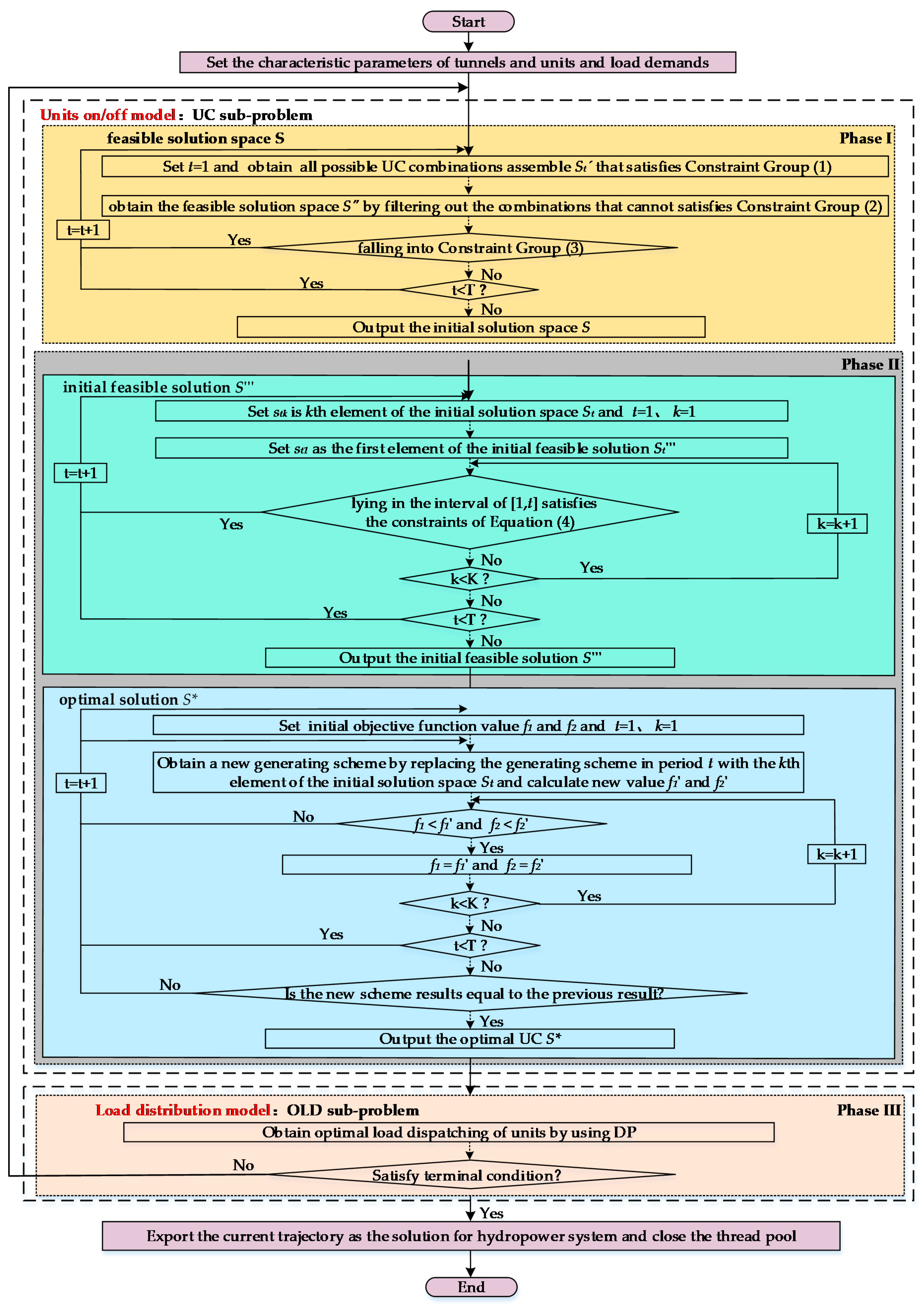
Figure 2 describes the detailed process of the two-phase decomposition approach for solving the STLD of the HPMTT problem. The flowchart is summarized below:
Step 1: Set the characteristic parameters of the tunnels and units, and load demands.
Step 2: Obtain a feasible solution space S of UC subproblem in Phase I.
Step 3: Obtain the initial feasible solution of the UC subproblem using the heuristic strategy in Phase II.
Step 4: POA uses the simplified dynamic programming recursive equation to solve the optimal solution of the UC subproblem in Phase II.
Step 5: Obtain the optimal result of the OLD subproblem using DP in Phase III.
Step 6: If the water consumption does not satisfy the terminal condition, return to Step 2; otherwise, export the current trajectory as the solution for the hydropower system and close the thread pool.
4. Case Study
4.1. Introduction of the Engineering Background and Setting the Parameters
The two-phase decomposition approach is applied to solve STLD for the HPMTT problem of the TSQII to evaluate its practicality. TSQII is located on the upstream of Nanpanjiang–Hongshui River, Guangxi Province, in southwestern China. The Hongshui River Cascade Hydropower Base is one of the 13 major hydropower bases in China and is an important energy base in South China. The Hongshui River flows from northwest to southeast with a length of approximately 1050 km, and it has a drainage area of 190,000 km2 and a natural drop of 762 m. As a region with abundant water energy resources in China, 11 cascaded hydropower stations for the main upstream of Hongshui River have been put into operation. Combined with the Datengxia Hydropower Station under construction, the mainstream has a total cascade generating capacity of 13,645 MW. Among the plants, TSQII is second, containing six main generating units with three different tunnels and an installed capacity of 1320 MW. The #1 and #2 units, #3 and #4 units, and #5 and #6 units are located in tunnels A, B, and C, respectively. TSQII is a daily regulating storage reservoir and is very sensitive to the change of water head. The head change directly impacts vibration zones dynamically and cannot be overlooked. TSQII is one of the main power plants for the West-to-East Electricity Transmission Project and has a significant role in frequency control and peak load regulation tasks. TSQII clearly reflects the characteristics of a HPMTT, which has greatly increased the difficult of modeling and optimization. A real-time operation example that incorporates different typical load rates in the dry season is developed.
Figure 3 plots different typical load rates for TSQII with a 96-point schedule, which has a single peak of 0.5 and a double peak of 0.29. During the wet season, there is abundant flood inflow in the Hongshui River. To avoid unnecessary spill flow and make full use of natural water resources, TSQII should generate has much power energy as possible. As a result, all of the units in different tunnels will be full-load operation.
Table 2 shows the unit characteristics of TSQII. The initial dam water level for dry season is 642.18 m, and the minimum uptime/downtime are assumed to be 1 hour. Integrated operation characteristic curves of the units are shown in Figure 4. Figure 5 shows the relationship curve of penstock head loss for TSQII. With the increase of the power release, the penstock head loss changes exponentially.
4.2. Analysis of Water Consumption for Different Startup Modes
A comparison of a turbine in one tunnel and two turbines in one tunnel is shown in Table 3. The actual load demand is 652.6 MW, and the load rate is 0.49. A single-period (15min) is used as an example for analysis. From Table 3, a turbine in one tunnel can achieve better total water consumption than two turbines in one tunnel. The total power release is 371.4 m3/s, and the optimal water consumption is 3.34 × 10⁵ m3. Meanwhile, the average head loss of tunnel B is 4.14 m, and the average water consumption rate is 2.05 m3/(kWh) for a turbine in one tunnel, in which the optimal startup mode is #1 for tunnel A, #4 for tunnel B, and #6 for tunnel C. The total power release is 393.4 m3/s and the optimal water consumption is 3.54 × 10⁵ m3. On the other hand, the average head loss of tunnel B is 19.62 m, and the average water consumption rate is 2.17 m3/(kWh) for two turbines in one tunnel, in which the optimal startup mode is #1 for tunnel A, and #3 and #4 for tunnel B. As a result, the single period water consumption decreased by 2 × 10⁴ m3, and the total water consumption decreased by 1.92 × 10⁶ m3. The scheduling results show a significant benefit for the daily regulating storage reservoir with high water head.
4.3. Comparison of Homogeneous Dispatch and TSM
A comparison of the results obtained from homogeneous dispatch, which distributes the load demand evenly to units of different tunnels, and TSM is presented in Table 4. It is clear that TSM can get better scheduling results than homogeneous dispatch. In dry season with high-rate load, the homogeneous dispatch fell into the vibration zone operation 51 times and the total water consumption is 3.75 × 10⁷ m3; the TSM fell into the vibration zone operation 0 times and the total water consumption is 2.70 × 10⁷ m3. Further, in dry season with low-rate load, the homogeneous dispatch fell into the vibration zone operation 34 times and the total water consumption is 2.93 × 10⁷ m3; the TSM fell into the vibration zone operation 0 times and the total water consumption is 2.01 × 10⁷ m3. These compared results fully demonstrate that the TSM is efficient for solving STLD for HPMTT problem while considering various constrains, and can get higher quality solutions with lower total water consumption.
4.4. On/Off Status of Units and Tunnel Analysis
With the initial conditions and parameters set in Section 4.1, the proposed heuristic searching method and progressive optimal algorithm are applied to obtain the on/off status of the units and tunnels. Table 5 shows the corresponding UC schedule of dry season with high-rate load. As shown, with the multiperiod optimization process based on POA in Section 3.4, the proposed algorithm can reasonably arrange the order of unit startup and shutdown and avoid frequent unit startup/shutdown. The water consumption of unit startup/shutdown is obtained as 7200 m3. There are four different schedules in Table 5: Two units operating from period 1 to 31 and period 84 to 96, four units operating from period 33 to 34 and period 54 to 82, five units operating from period 35 to 53 during high load, and three units for the other periods. Taking period 32 to 35 as an example, the power generation increased from 466.1 MW to 876.1 MW to respond to system demands. The number of startup units increased from three units to five units in order to connect the startup mode between periods. The three units operating included #1 for tunnel A, #3 for tunnel B, and #6 for tunnel C. Furthermore, when the load demands sharply decrease, the number of startup units correspondingly decrease. Power generation decreased from 646.1 MW to 428.5 MW to respond to system demands from period 83 to 84, and the number of startup units decreased from three units to two units.
The unit on/off states in dry season with low-rate load are shown in Table 6. The load demands were lower than during dry season with high-rate load; thus, startup/shutdown was more frequent than during dry season with high-rate load. Simultaneously, the water consumption of unit startup/shutdown increased to 14,400 m3. Correspondingly, to meet the peak load regulation task of the hydropower plant, four units operated from period 41 to 56 and period 71 to 85. During the other periods, the number of startup units was less than 4 and included a turbine in one-tunnel mode in order to make full use of water energy and reduce water consumption.
4.5. Simulation Results and Analysis for Dry Season with High-Rate Load
A unit must operate within its feasible generation range and avoid operation in the forbidden zones for that unit. The possible combining vibration zones must be known to determine the optimal scheduling. Table 7 lists the combined vibration zones for different combinations of generating units. The startup mode falls easily into the vibration zones in each period when the load demands change.
The load dispatch results of the units during dry season with high-rate loads are shown in Figure 6. As shown, the load dispatch results during dry season with high-rate loads easily fall into peak output due to the frequent change of load demands and vibration zone constraints. Using period 32 to 33 as an example, the power generation values fluctuated from 466.1 MW to 690.2 MW. Meanwhile, the load dispatch for each unit must be carefully determined because of the previous power output and varied constraints, which is the reason the power output of #1 for tunnel A slightly decreases in period 32. To respond promptly to peak loads and vibration zone constraints from period 34 to 82, it is significant and necessary to increase the number of startup units. In this case, the power output of each unit for each interval obviously meets the vibration zone limits, which indicates that the power output avoidance strategy proposed in Section 3.5 is effective.
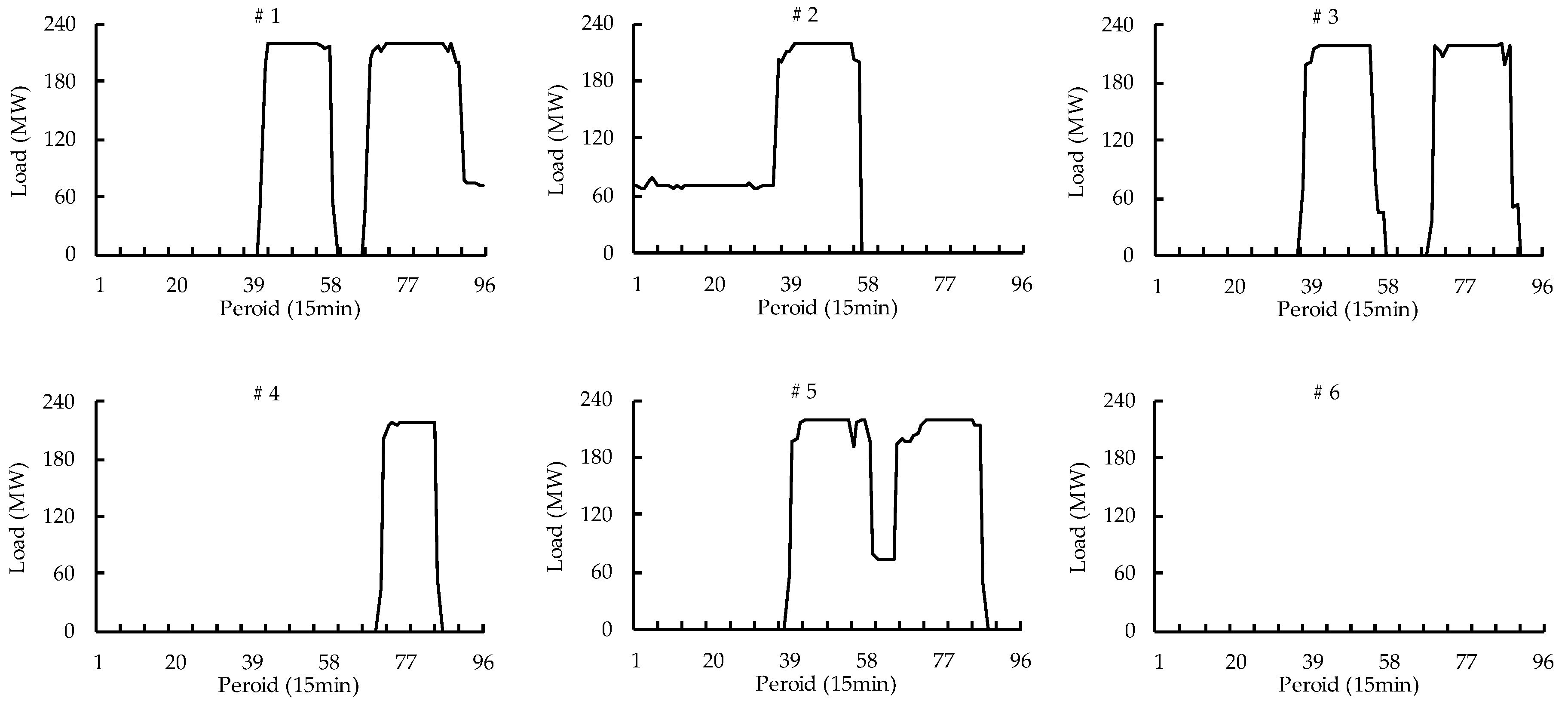
4.6. Simulation Results and Analysis for Dry Season with Low-Rate Load
Figure 7 shows the load dispatch results for the dry season with a low-rate load. As shown, the power output obtained by the proposed two-stage model meets all of the constraints. As shown in Figure 7, the unit output fluctuates substantially as the load demands frequently fluctuate. For the period from 41 to 60, the power generation values fluctuate from 685.3 to 78.3 MW, and the number of units fluctuates from 4 to 1. Essentially, the load dispatch for each period must be carefully performed due to varied vibration zones. From Figure 7, the OLD subproblem successfully avoided the complex vibration zones by using the two-phase decomposition approach in this paper. Accordingly, there were six different ranges: Range 1 (period 1 to 36), range 2 (period 41 to 56), range 3 (period 60 to 66), range 4 (period 71 to 85), range 5 (period 91 to 96), and range 6 (other periods). One unit operated in range 1, range 3, and range 5 while satisfying the minimum uptime/downtime constraints and avoiding vibration zones. Four units operated in range 2 and range 4 because of higher load demands. For range 6, the number of startup units is less than 4, and the startup mode is a turbine in one tunnel.
5. Conclusions
In this paper, the TSM is proposed to effectively solve STLD for HPMTT problems, which is composed of a unit on/off model and a load distribution model. The significant innovations of the proposed method mainly include the following three points: (1) STLD for a HPMTT problem is decomposed into the subproblems of UC and OLD; (2) the unit on/off model, the new mathematical model, is proposed to solve the UC subproblem by a heuristic searching method and a progressive optimal algorithm; (3) the DP is used to solve the OLD subproblem, which is based on a fixed startup mode. Finally, the simulation results reveal that total water consumption of optimal dispatch can save a higher amount of water consumption than homogeneous dispatch. In conclusion, this paper proposes a new mathematical model that can achieve safe hydropower and economic operation. Furthermore, the successful applications of the proposed model demonstrate its utility and efficiency for solving the STLD for a HPMTT problem, such as the TSQII in the dry season under different typical load rates.
Author Contributions
S.L. carried out the study design, the analysis and interpretation of data, and drafted the manuscript. H.Z. participated in the study design, data collection, analysis of data, and preparation of the manuscript. G.L. and S.L. carried out the experimental work and the data collection and interpretation. B.L. participated in the design and coordination of experimental work, and acquisition of data. All authors read and approved the final manuscript.
Funding
This research was funded by National Natural Science Foundation of China grant number U1765103 and the Liaoning province Natural Science Foundation of China grant number 20180550354.
Conflicts of Interest
The authors declare no conflict of interest.
References
- Feng, Z.K.; Niu, W.J.; Cheng, C.T. Optimizing electrical power production of hydropower system by uniform progressive optimality algorithm based on two-stage search mechanism and uniform design. J. Clean. Prod. 2018, 190, 432–442. [Google Scholar] [CrossRef]
- Cheng, C.T.; Liao, S.L.; Tang, Z.T.; Zhao, M.Y. Comparison of particle swarm optimization and dynamic programming for large scale hydro unit load dispatch. Energy Conv. Manag. 2009, 50, 3007–3014. [Google Scholar] [CrossRef]
- Han, J.C.; Huang, G.H.; Zhang, H.; Zhuge, Y.S.; He, L. Fuzzy constrained optimization of eco-friendly reservoir operation using self-adaptive genetic algorithm: A case study of a cascade reservoir system in the Yalong River, China. Ecohydrology 2012, 5, 768–778. [Google Scholar] [CrossRef]
- Rezghi, A.; Riasi, A. The interaction effect of hydraulic transient conditions of two parallel pump-turbine units in a pumped-storage power plant with considering “S-shaped” instability region: Numerical simulation. Renew. Energy 2018, 118, 896–908. [Google Scholar] [CrossRef]
- Xu, B.B.; Wang, F.F.; Chen, D.Y.; Zhang, H. Hamiltonian modeling of multi-hydro-turbine governing systems with sharing common penstock and dynamic analyses under shock load. Energy Conv. Manag. 2016, 108, 478–487. [Google Scholar] [CrossRef]
- Arul, R.; Ravi, G.; Velusami, S. An improved harmony search algorithm to solve economic load dispatch problems with generator constraints. Electr. Eng. 2014, 96, 55–63. [Google Scholar] [CrossRef]
- Alvarez, G.E.; Marcovecchio, M.G.; Aguirre, P.A. Security-constrained unit commitment problem including thermal and pumped storage units: An MILP formulation by the application of linear approximations techniques. Electr. Power Syst. Res. 2018, 154, 67–74. [Google Scholar] [CrossRef]
- Fersi, M.; Triki, A. Investigation on redesigning strategies for water-hammer control in pressurized-piping systems. J. Press. Vessel Technol. 2019, 141, 021301. [Google Scholar] [CrossRef]
- Ghidaoui, M.S.; Zhao, M.; McInnis, D.A.; Axworthy, D.H. A review of water hammer theory and practice. Appl. Mech. Rev. 2005, 58, 49–76. [Google Scholar] [CrossRef]
- Nemati, M.; Braun, M.; Tenbohlen, S. Optimization of unit commitment and economic dispatch in microgrids based on genetic algorithm and mixed integer linear programming. Appl. Energy 2018, 210, 944–963. [Google Scholar] [CrossRef]
- Kumar, D.N.; Reddy, M.J. Ant colony optimization for multi-purpose reservoir operation. Water Resour. Manag. 2006, 20, 879–898. [Google Scholar] [CrossRef]
- Dubey, H.M.; Pandit, M.; Panigrahi, B.K. Ant lion optimization for short-term wind integratedhydrothermal power generation scheduling. Int. J. Electr. Power Energy Syst. 2016, 83, 158–174. [Google Scholar] [CrossRef]
- Lu, P.; Zhou, J.Z.; Wang, C.; Qiao, Q.; Mo, L. Short-term hydro generation scheduling of Xiluodu and Xiangjiaba cascade hydropower stations using improved binary-real coded bee colony optimization algorithm. Energy Conv. Manag. 2015, 91, 19–31. [Google Scholar] [CrossRef]
- Rasoulzadeh-Akhijahani, A.; Mohammadi-Ivatloo, B. Short-term hydrothermal generation scheduling by a modified dynamic neighborhood learning based particle swarm optimization. Int. J. Electr. Power Energy Syst. 2015, 67, 350–367. [Google Scholar] [CrossRef]
- Kumar, D.N.; Reddy, M.J. Multipurpose reservoir operation using particle swarm optimization. J. Water Resour. Plan. Manag. 2007, 133, 192–201. [Google Scholar] [CrossRef]
- Lee, H.; Maravelias, C.T. Discrete-time mixed-integer programming models for short-term scheduling in multipurpose environments. Comput. Chem. Eng. 2017, 107, 171–183. [Google Scholar] [CrossRef]
- Guedes, L.S.M.; Maia, P.D.M.; Lisboa, A.C.; Vieira, D.A.G.; Saldanha, R.R. A unit commitment algorithm and a compact MILP model for short-term hydro-power generation scheduling. IEEE Trans. Power Syst. 2017, 32, 3381–3390. [Google Scholar] [CrossRef]
- Borghetti, A.; D’Ambrosio, C.; Lodi, A.; Martello, S. An MILP approach for short-term hydro scheduling and unit commitment with head-dependent reservoir. IEEE Trans. Power Syst. 2008, 23, 1115–1124. [Google Scholar] [CrossRef]
- Li, X.; Li, T.J.; Wei, J.H.; Wang, G.Q.; Yeh, W.W.G. Hydro unit commitment via mixed integer linear programming: A case study of the three gorges project, China. IEEE Trans. Power Syst. 2014, 29, 1232–1241. [Google Scholar] [CrossRef]
- Pérez, D.J.; Wilhelmi, J.R.; Arévalo, L.A. Optimal short-term operation schedule of a hydropower plant in a competitive electricity market. Energy Convers. Manag. 2010, 51, 2955–2966. [Google Scholar] [CrossRef]
- Bhullar, S.; Ghosh, S. Optimal integration of multi distributed generation sources in radial distribution networks using a hybrid algorithm. Energies 2018, 11, 628. [Google Scholar] [CrossRef]
- Rajan, C.C.A. Hydro-thermal unit commitment problem using simulated annealing embedded evolutionary programming approach. Int. J. Electr. Power Energy Syst. 2011, 33, 939–946. [Google Scholar] [CrossRef]
- Finardi, E.C.; Scuzziato, M.R. Hydro unit commitment and loading problem for day-ahead operation planning problem. Int. J. Electr. Power Energy Syst. 2013, 44, 7–16. [Google Scholar] [CrossRef]
- Liao, S.L.; Li, Z.F.; Li, G.; Wang, J.Y.; Wu, X.Y. Modeling and optimization of the medium-term units commitment of thermal power. Energies 2015, 8, 12848–12864. [Google Scholar] [CrossRef]
- Moradi, H.; Alasty, A.; Vossoughi, G. Nonlinear dynamics and control of bifurcation to regulate the performance of a boiler-turbine unit. Energy Conv. Manag. 2013, 68, 105–113. [Google Scholar] [CrossRef]
- Zhu, H.; Huang, G.H. Dynamic stochastic fractional programming for sustainable management of electric power systems. Int. J. Electr. Power Energy Syst. 2013, 53, 553–563. [Google Scholar] [CrossRef]
- Yan, D.L.; Wang, W.Y.; Chen, Q.J. Nonlinear modeling and dynamic analyses of the hydro–turbine governing system in the load shedding transient regime. Energies 2018, 11, 1244. [Google Scholar] [CrossRef]
- Tijsseling, A.S. Water hammer with fluid–structure interaction in thick-walled pipes. Comput. Struct. 2007, 85, 844–851. [Google Scholar] [CrossRef] [Green Version]
- Yang, W.J.; Yang, J.D.; Guo, W.C.; Zeng, W.; Wang, C.; Saarinen, L.; Norrlund, P. A mathematical model and its application for hydro power units under different operating conditions. Energies 2015, 8, 10260–10275. [Google Scholar] [CrossRef]
- Gabl, R.; Gems, B.; Birkner, F.; Aufleger, M. Adaptation of an existing intake structure caused by increased sediment level. Water 2018, 10, 1066. [Google Scholar] [CrossRef]
- Bermudez, M.; Cea, L.; Puertas, J.; Conde, A.; Martin, A.; Baztan, J. Hydraulic model study of the intake-outlet of a pumped-storage hydropower plant. Eng. Appl. Comp. Fluid Mech. 2017, 11, 483–495. [Google Scholar] [CrossRef] [Green Version]
- Khan, L.; Wicklein, E.; Rashid, M.; Ebner, L.; Richards, N. Computational fluid dynamics modeling of turbine intake hydraulics at a hydropower plant. J. Hydraul. Res. 2004, 42, 61–69. [Google Scholar] [CrossRef]
Figure 1.
Sketch of hydropower plant with multiple turbines in one tunnel (HPMTT) with long diversion system.
Figure 1.
Sketch of hydropower plant with multiple turbines in one tunnel (HPMTT) with long diversion system.
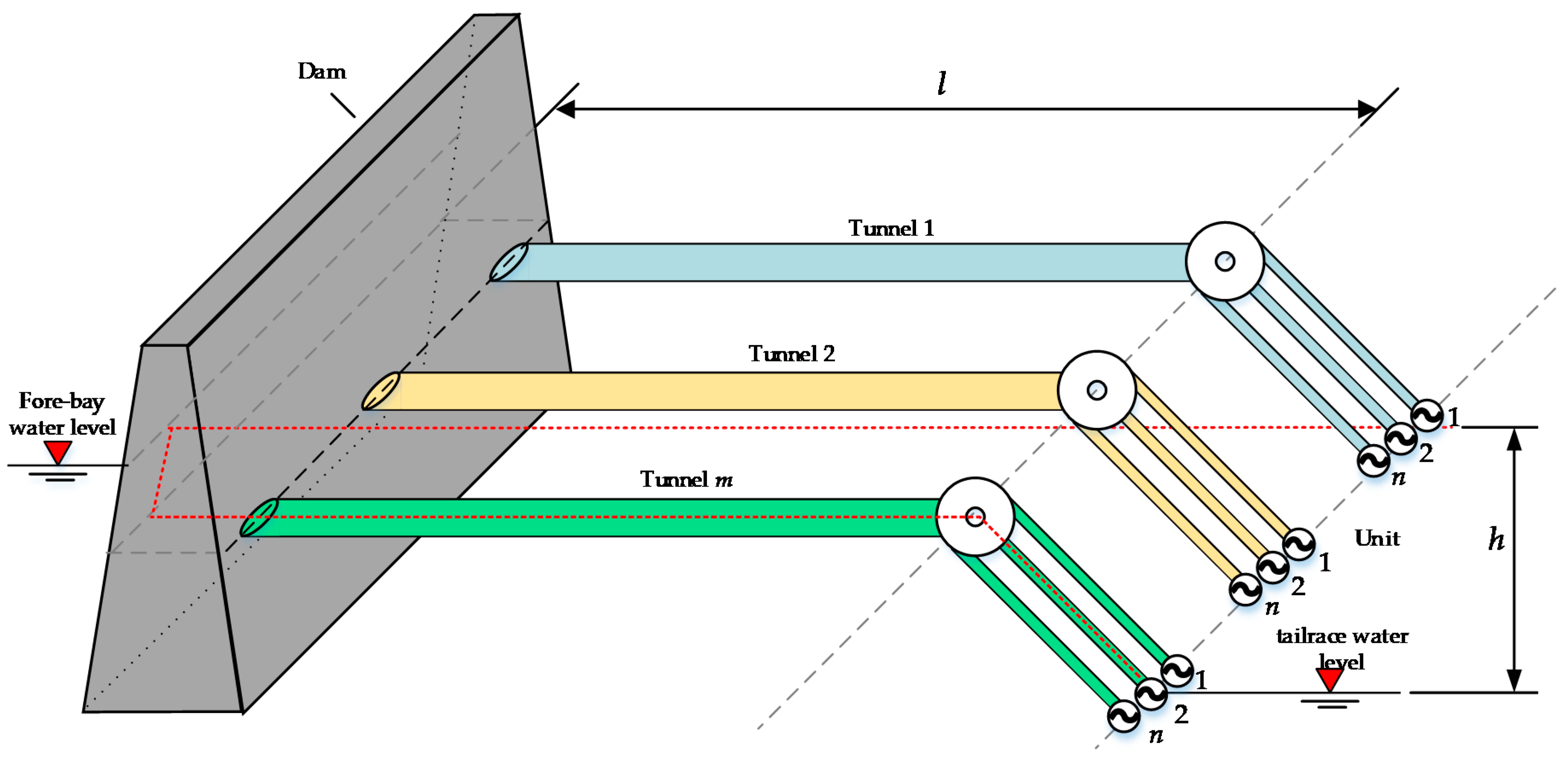
Figure 2.
Flowchart of two-phase decomposition approach for solving short-term load dispatching (STLD).
Figure 2.
Flowchart of two-phase decomposition approach for solving short-term load dispatching (STLD).

Figure 3.
Daily schedules of dry season with different typical load rates.
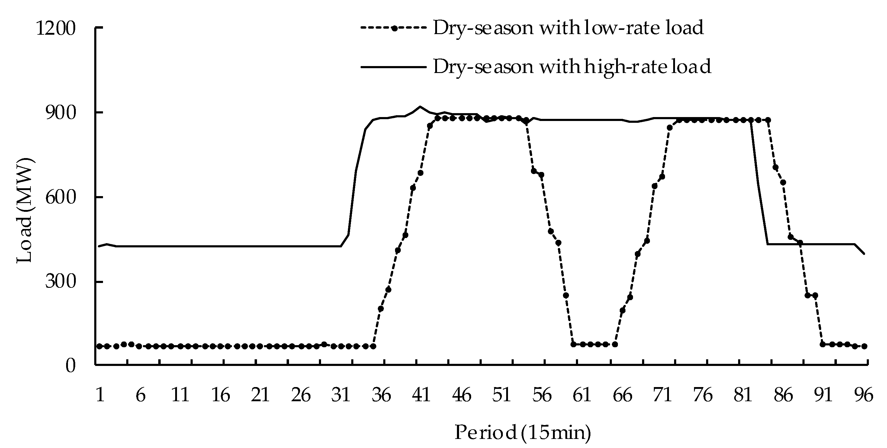
Figure 4.
Operation characteristic curves of units for different work water head.
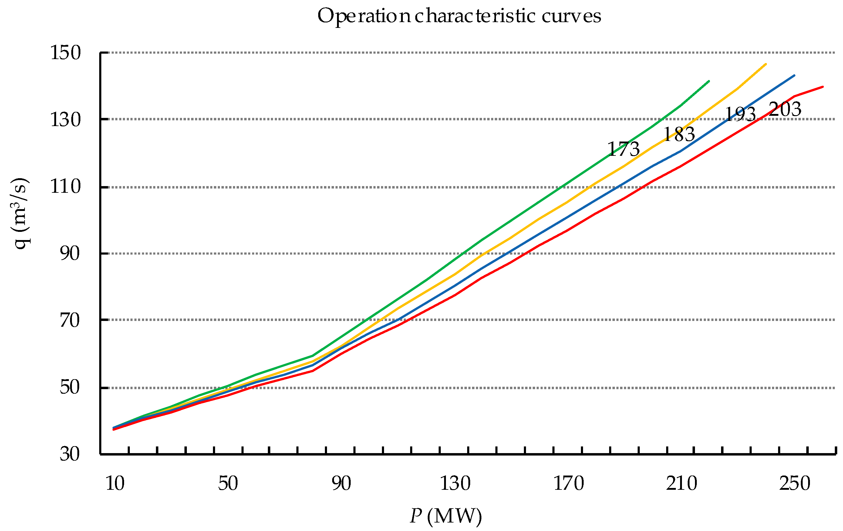
Figure 5.
Relationship curve of penstock head loss for Tianshengqiao-II reservoir (TSQII).
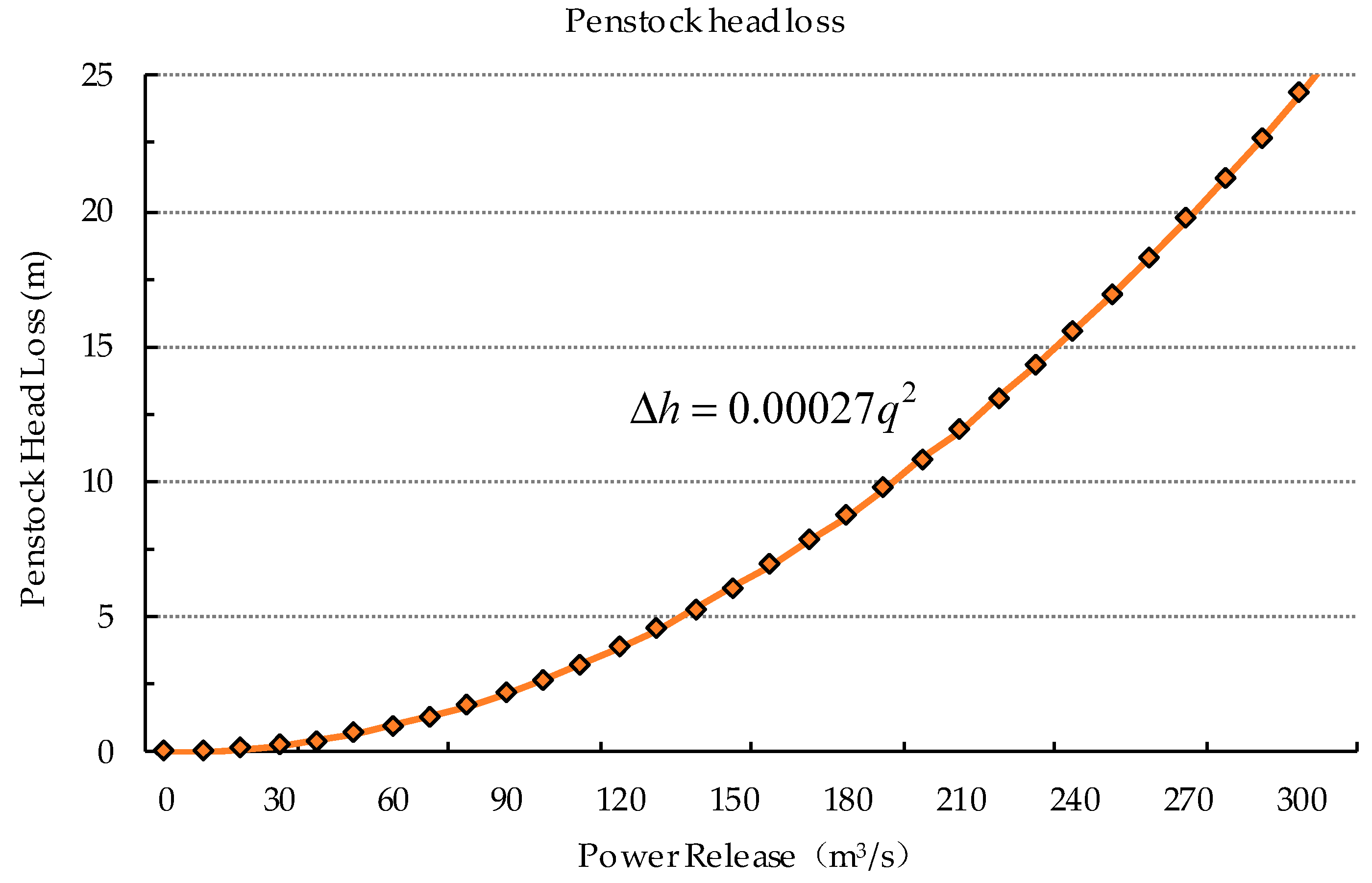
Figure 6.
Load dispatch results of #1–#6 for dry season with high-rate load.
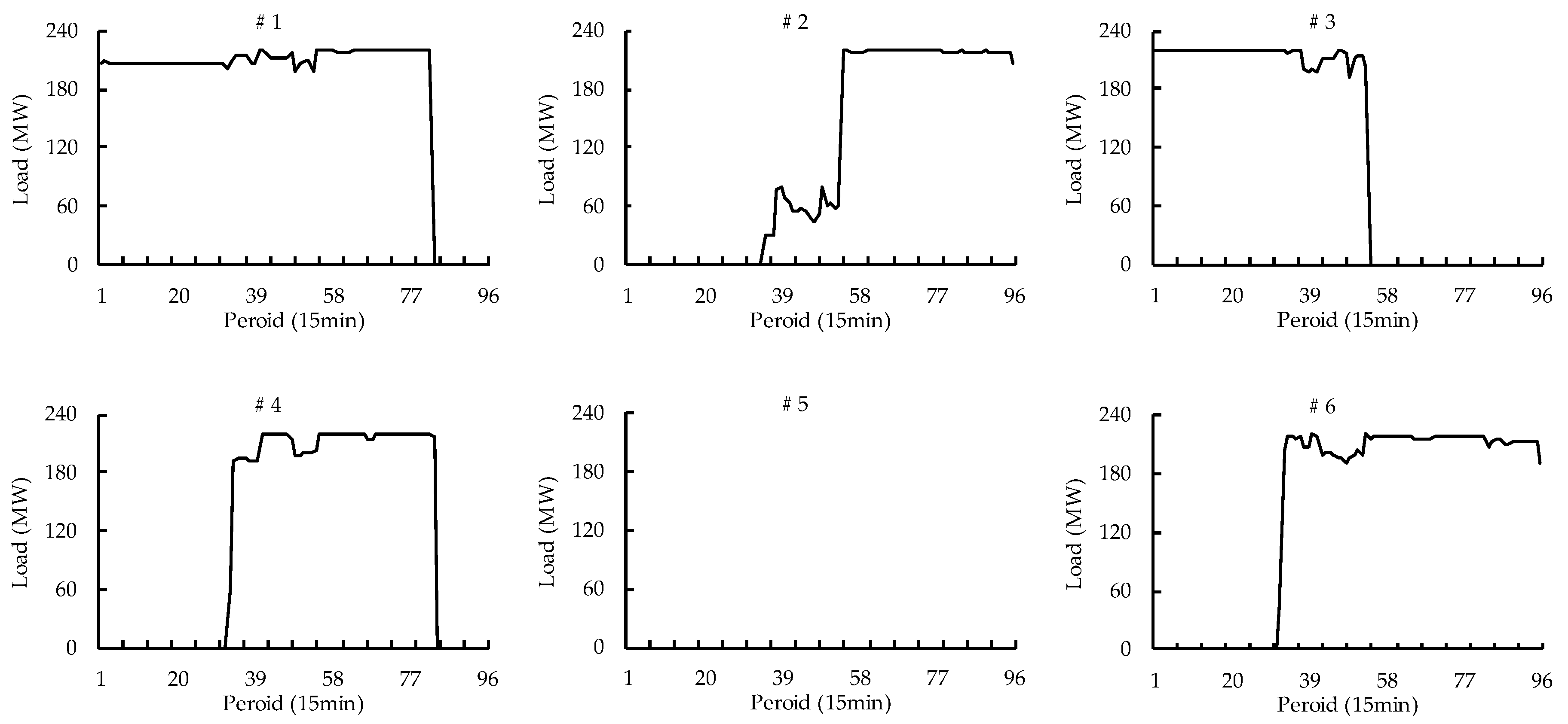
Figure 7.
Load dispatch results of #1–#6 for dry season with low-rate load.

Table 1.
Unit parameters of typical hydropower plants.
| Power Station | TSQII | Jinping II | Lubuge |
|---|---|---|---|
| Total installed capacity (MW) | 1320 | 4800 | 600 |
| Length of tunnel (km) | 9.77 | 16.67 | 9.38 |
| Average head (m) | 176 | 290 | 327.7 |
| Number of tunnels | 3 | 4 | 1 |
| Number of units | 2 | 2 | 3 |
Table 2.
Units’ characteristics of TSQII.
| Item | Value |
|---|---|
| Maximum water head (m) | 645.00 |
| Minimum water head (m) | 637.00 |
| Units (capacity × number, MW) | 220.0 × 6 |
| Vibration zones (MW) | (80,190) |
| Startup/Shutdown water consumption (m3) | 1200 |
| Discrete step of water level (m) | 0.1 |
| Initial dam water level for dry season (m) | 642.18 |
| Duration of online/offline of units | 4 |
| Scheduling period (min) | 15 |
| Parameter A of penstock head loss | 2.7 × 10⁻⁴ |
Table 3.
Comparison of a turbine in one tunnel and two turbines in one tunnel.
| Tunnel | Unit | Turbine in One Tunnel | Two Turbines in One Tunnel | ||||||
|---|---|---|---|---|---|---|---|---|---|
| Load (MW) | Power Release (m3/s) | Head Loss (m) | Water Consumption Rate (m3/(kWh)) | Load (MW) | Power Release (m3/s) | Head Loss (m) | Water Consumption Rate (m3/(kWh)) | ||
| A | #1 | 217.6 | 123.8 | 4.14 | 2.05 | 217.6 | 123.8 | 4.14 | 2.05 |
| #2 | 0 | 0 | - | 0 | 0 | - | |||
| B | #3 | 0 | 0 | 4.14 | - | 217.5 | 134.8 | 19.62 | 2.23 |
| #4 | 217.5 | 123.8 | 2.05 | 217.5 | 134.8 | 2.23 | |||
| C | #5 | 0 | 0 | 4.14 | - | 0 | 0 | 0 | - |
| #6 | 217.5 | 123.8 | 2.05 | 0 | 0 | - | |||
| Total value | 652.6 | 371.4 | - | 2.05 | 652.6 | 393.4 | - | 2.17 | |
Table 4.
Comparison of homogeneous dispatch and two-stage model (TSM).
| Item | Dry Season with High-Rate Load | Dry Season with Low-Rate Load | ||
|---|---|---|---|---|
| Homogeneous Dispatch | TSM | Homogeneous Dispatch | TSM | |
| Number of fell into vibration zone | 51 | 0 | 34 | 0 |
| Water consumption (m3) | 3.75 × 10⁷ | 2.70 × 10⁷ | 2.93 × 10⁷ | 2.01 × 10⁷ |
Table 5.
Unit state in dry season with high-rate load.
| Period | Load (MW) | Tunnel A | Tunnel B | Tunnel C | Total | Duration of Unit | |||
|---|---|---|---|---|---|---|---|---|---|
| #1 | #2 | #3 | #4 | #5 | #6 | ||||
| 1 | 427.5 | 1 | 0 | 1 | 0 | 0 | 0 | 2 | 31 |
| 32 | 466.1 | 1 | 0 | 1 | 0 | 0 | 1 | 3 | 1 |
| 33 | 690.2 | 1 | 0 | 1 | 1 | 0 | 1 | 4 | 2 |
| 35 | 876.1 | 1 | 1 | 1 | 1 | 0 | 1 | 5 | 19 |
| 54 | 857.6 | 1 | 1 | 0 | 1 | 0 | 1 | 4 | 29 |
| 83 | 646.1 | 0 | 1 | 0 | 1 | 0 | 1 | 3 | 1 |
| 84 | 428.5 | 0 | 1 | 0 | 0 | 0 | 1 | 2 | 13 |
| 96 | 397.5 | 0 | 1 | 0 | 0 | 0 | 1 | 2 | |
The water consumption of unit startup/shutdown is 7200 m3.
Table 6.
Unit state in dry season with low-rate load.
| Period | Load (MW) | Tunnel A | Tunnel B | Tunnel C | Total | The Duration of Unit | |||
|---|---|---|---|---|---|---|---|---|---|
| #1 | #2 | #3 | #4 | #5 | #6 | ||||
| 1 | 71.3 | 0 | 1 | 0 | 0 | 0 | 0 | 1 | 36 |
| 37 | 268.6 | 0 | 1 | 1 | 0 | 0 | 0 | 2 | 2 |
| 39 | 466.4 | 0 | 1 | 1 | 0 | 1 | 0 | 3 | 2 |
| 41 | 685.3 | 1 | 1 | 1 | 0 | 1 | 0 | 4 | 16 |
| 57 | 479.9 | 1 | 0 | 1 | 0 | 1 | 0 | 3 | 1 |
| 58 | 436.5 | 1 | 0 | 0 | 0 | 1 | 0 | 2 | 2 |
| 60 | 78.3 | 0 | 0 | 0 | 0 | 1 | 0 | 1 | 7 |
| 67 | 243.1 | 1 | 0 | 0 | 0 | 1 | 0 | 2 | 2 |
| 69 | 444.3 | 1 | 0 | 1 | 0 | 1 | 0 | 3 | 2 |
| 71 | 670 | 1 | 0 | 1 | 1 | 1 | 0 | 4 | 15 |
| 86 | 652.6 | 1 | 0 | 1 | 0 | 1 | 0 | 3 | 2 |
| 88 | 438.5 | 1 | 0 | 1 | 0 | 0 | 0 | 2 | 3 |
| 91 | 77.6 | 1 | 0 | 0 | 0 | 0 | 0 | 1 | 6 |
| 96 | 72.3 | 1 | 0 | 0 | 0 | 0 | 0 | 1 | |
The water consumption of units’ startup/shutdown is 14,400 m3.
Table 7.
UC combined vibration zones of TSQII (Water head 170 m).
| Combinations of Generating Units | Capacity Combination/MW | Combined Vibration Zones/MW |
|---|---|---|
| One unit | 220 | (80,190) |
| Two units | 440 | (160,190) ∪ (300,380) |
| Three units | 660 | (520,570) |
| Four units | 880 | (740,760) |
| Five units | 1100 | Vibration-free Zone |
| Six units | 1320 | Vibration-free Zone |
© 2019 by the authors. Licensee MDPI, Basel, Switzerland. This article is an open access article distributed under the terms and conditions of the Creative Commons Attribution (CC BY) license (http://creativecommons.org/licenses/by/4.0/).
Share and Cite
MDPI and ACS Style
Liao, S.; Zhao, H.; Li, G.; Liu, B. Short-Term Load Dispatching Method for a Diversion Hydropower Plant with Multiple Turbines in One Tunnel Using a Two-Stage Model. Energies 2019, 12, 1476. https://doi.org/10.3390/en12081476
AMA Style
Liao S, Zhao H, Li G, Liu B. Short-Term Load Dispatching Method for a Diversion Hydropower Plant with Multiple Turbines in One Tunnel Using a Two-Stage Model. Energies. 2019; 12(8):1476. https://doi.org/10.3390/en12081476
Chicago/Turabian StyleLiao, Shengli, Hongye Zhao, Gang Li, and Benxi Liu. 2019. "Short-Term Load Dispatching Method for a Diversion Hydropower Plant with Multiple Turbines in One Tunnel Using a Two-Stage Model" Energies 12, no. 8: 1476. https://doi.org/10.3390/en12081476
Note that from the first issue of 2016, this journal uses article numbers instead of page numbers. See further details here.