Combined Effect of Rotational Augmentation and Dynamic Stall on a Horizontal Axis Wind Turbine


Jiangsu Key Laboratory of Hi-Tech Research for Wind Turbine Design, Nanjing University of Aeronautics and Astronautics, Nanjing 210016, China
*
Author to whom correspondence should be addressed.
Energies 2019, 12(8), 1434; https://doi.org/10.3390/en12081434
Submission received: 20 March 2019
/
Revised: 9 April 2019
/
Accepted: 11 April 2019
/
Published: 14 April 2019
(This article belongs to the Special Issue Recent Advances in Aerodynamics of Wind Turbines)
Abstract
:Rotational augmentation and dynamic stall have been extensively investigated on horizontal axis wind turbines (HAWTs), but usually as separate topics. Although these two aerodynamic phenomena mainly determine the unsteady loads and rotor performance, the combined effect of rotational augmentation and dynamic stall is still poorly understood and is challenging to model. We perform a comprehensive comparative analysis between the two-dimensional (2D) airfoil flow and three-dimensional (3D) blade flow to provide a deep understanding of the combined effect under yawed inflow conditions. The associated 2D aerodynamic characteristics are examined by the unsteady Reynolds-averaged Navier-Stokes Simulations, and are compared with the experimental data of NREL Phase VI rotor in three aspects: aerodynamic hysteresis, flow field development, and dynamic stall regimes. We find that the combined effect can dramatically reduce the sectional lift and drag hysteresis by almost 60% and 80% from the supposed definitions of hysteresis intensity, and further delay the onset of stall compared with either of rotational augmentation and dynamic stall. The flow field development analysis indicates that the 3D separated flow is greatly suppressed in the manner of changing the massive trailing-edge separation into the moderate leading-edge separation. Furthermore, the 3D dynamic stall regime indicates a different stall type and an opposite trend of the separated zone development, compared with the 2D dynamic stall regime. These findings suggest that the modelling of 3D unsteady aerodynamics should be based on the deep understanding of 3D unsteady blade flow rather than correcting the existing 2D dynamic stall models. This work is helpful to develop analytical models for unsteady load predictions of HAWTs.
1. Introduction
Horizontal axis wind turbines (HAWTs) often experience unsteady aerodynamic loads, to which wind turbine failure, reduced machine life, and increased operating maintenance are all directly linked. Subjected to inevitable wind direction fluctuations in the atmosphere and yaw system failure, the direction of HAWT rotation commonly misaligns with the wind direction [1]. Consequently, the associated azimuthal variation of the aerodynamic loads can fatigue turbine structures, and the output power is expected to decrease with resulting economical loss [2]. However, the modelling of yaw aerodynamics and accurate prediction of the unsteady loads face many challenges [1,2,3]. This is mainly because the blade flow field is unsteady and three-dimensional (3D) with the separated flow. The unsteadiness can bring about dynamic stalls accompanied by great load variations [4]; meanwhile, the 3D effects like finite span, rotational augmentation, and local sweep effect, can make the blade flow highly complicated [3,5]. Particularly, the combined effect of rotational augmentation and dynamic stall plays an essential role in the 3D boundary layer development and hence the aerodynamic characteristics [5].
During the last few decades, both dynamic stall and rotational augmentation have captured significant attention, but have usually been studied independently. Plenty of fundamental investigations of dynamic stall and rotational augmentation, including the wind tunnel experiments, computational fluid dynamics (CFD) simulations, and analytical modellings, have shed light on the flow mechanisms separately. Dynamic stall is often studied on two-dimensional (2D) wind turbine airfoils undergoing sinusoidal pitch oscillation about the quarter-chord axis [6]. Dynamic stall is characterized by the shedding and passage of a strong vortical disturbance over the suction surface, inducing a highly nonlinear fluctuating pressure field [7,8]. Rotational augmentation is, however, often studied on 3D blades under the axial inflow conditions. The underlying principle lies in the centrifugal and Coriolis forces due to rotation. The centrifugal force can result in radial flow and then generate the chordwise Coriolis force which counteracts the adverse pressure gradient, flattens the separated zone, and eventually, elevates the aerodynamic forces [9,10,11,12]. Bangga [13] conducted a comprehensive study of the rotational augmentation on stall-controlled and pitch-regulated HAWTs. It should be noted that both dynamic stall and rotational augmentation can delay the onset of stall, based on the aforementioned different flow mechanisms. To consider these two significant phenomena in the rotor design process, several analytical models have been proposed separately [14,15]. However, they often lack rigor and generality, particularly when the nonlinear aerodynamic responses are predominant at the high angle of attack (AOA).
So far the conventional approach to predicting the unsteady loads on yawed HAWTs is to use the rotational augmentation models and dynamic stall models in sequence, as described in the well-known blade-element momentum (BEM) code of FAST V8 [16,17]. Although both the rotational augmentation model and dynamic stall model were included, the BEM method and vortex wake method produced poor results, particularly at the inboard blade sections [18,19]. This is attributable to the improper consideration of the combined effect of rotational augmentation and dynamic stall. In contrast, the CFD method has shown a potential in capturing the 3D unsteady aerodynamic characteristics [20,21]. Schreck and Robinson [22] have investigated rotational augmentation and dynamic stall on the NREL Phase VI rotor, based on the plenty of wind tunnel experimental data. The dynamic stall vortex initiation and convection were discussed in details to point out the highly 3D and unsteady flow characteristics. Nevertheless, flow mechanisms of the combined effect have not yet been well understood or analytically modelled.
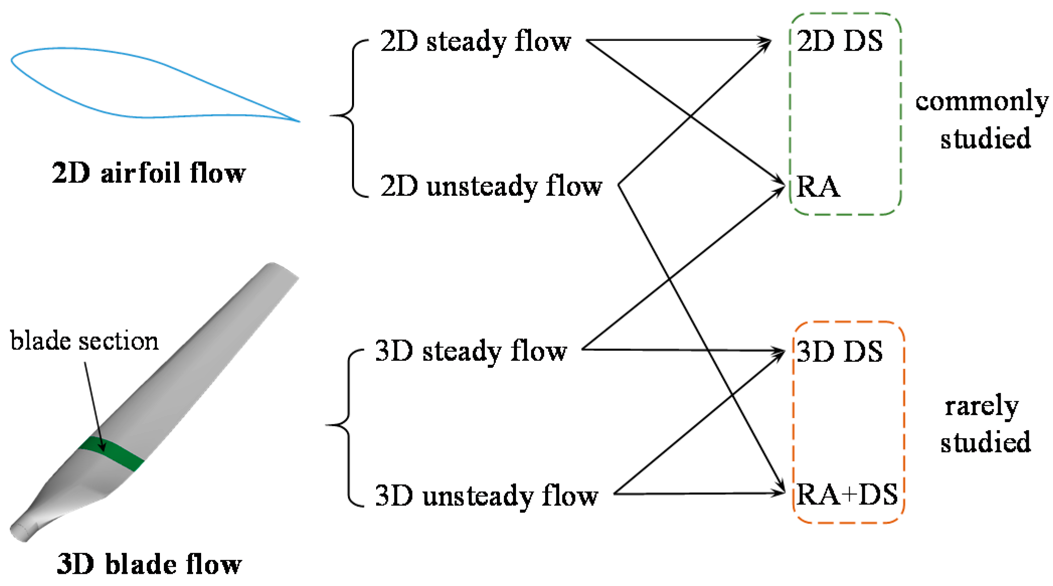
Figure 1 gives a schematic diagram of the comparative studies between 2D airfoil flow and 3D blade flow. The idea is to isolate the influence of rotational augmentation or dynamic stall by means of the comparative analyses. Plenty of comparative studies have been carried out on the 2D dynamic stall and rotational augmentation [6,23,24,25]. The 3D dynamic stall combined with rotational augmentation is, however, rarely studied. To provide a deep understanding of the combined effect of rotational augmentation and dynamic stall under yawed inflow conditions, this article presents a comparative study between the 2D unsteady airfoil flow and 3D unsteady blade flow, similar to the common strategy for steady aerodynamics. The available experimental data from [26,27] are used for the 2D steady flow, 3D steady flow, and 3D unsteady flow. The sectional inflow velocity and AOA variations are extracted from the 3D experimental data [27] using the inverse BEM approach. The aerodynamic characteristics of 2D unsteady flow are examined by the unsteady Reynolds-averaged Navier-Stokes Simulations (URANS) in the present work.
In this study, the combined effect is found to favorably reduce the aerodynamic hysteresis, and further delay the onset of stall compared with either of rotational augmentation and dynamic stall. The 3D dynamic stall regime indicates a different stall type and an opposite trend of the separated zone development, compared with the 2D dynamic stall regime. This study provides insight into the flow mechanisms of the combined effect of rotational augmentation and dynamic stall. The comparative analysis is expected to improve the understanding and modelling of yaw aerodynamics, and hence the predictive accuracy of unsteady aerodynamic loads on HAWTs.
2. Yaw Aerodynamics
Since the so-called strip theory is commonly applied to engineering tools, the yaw aerodynamics are determined on blade sections to compare the sectional aerodynamic responses with the 2D airfoil aerodynamics. Figure 2 gives the definitions of yaw angle ϕy and azimuth angle ϕa. In this work, the blade azimuth is defined zero at 6 o’clock position, and the rotor is assumed to rotate clockwise.
Figure 3a shows the relation between in-plane and out-plane velocity components. From this figure, we can obtain the following formulae of local AOA α and resultant velocity Vr at blade sections:
where Vw, vai, vti, Ω, r and θ are the wind speed, axial induced velocity, tangential induced velocity, rotor speed, radial location and blade pitch angle plus local twist angle, respectively. The tangential induced velocity vti is often negligible. Figure 3b gives the relation among aerodynamic forces referred to three orthogonal coordinate systems. Their relation can be formulated as follows:
where N, T, L, D, Th and Tq are the normal force, tangential force, lift force, drag force, and forces perpendicular and tangential to the rotor plane, respectively. These aerodynamic forces can be further nondimensionalized with the local dynamic pressure and chord length c.
L = Ncosα + Tsinα
D = Nsinα − Tcosα
D = Nsinα − Tcosα
Th = Ncosθ − Tsinθ
Tq = Nsinθ + Tcosθ
Tq = Nsinθ + Tcosθ
There are two important factors in yaw aerodynamics. First, the skewed wake geometry can result in an azimuthal variation of the induced velocity, because the proximity to the wake vortices strongly influences the inflow. According to the Biot-Savart law, the trailing tip vorticity is closer to the downwind side of rotor plane (Figure 2a), leading to a higher value of the axial induced velocity vai. From Equation (1), the skewed wake geometry has a strong impact on local AOA, particularly at low wind speed. The asymmetrical axial velocity and AOA distributions will further cause a load unbalance and determine the yawing stability. Second, the blade will be retreating in the upper half plane and advancing in the lower half plane at positive yaw angles (Figure 2b). This effect lies in the in-plane wind speed component, Vwsinϕycosϕa. It can yield the noticeable azimuthal variations of the local AOA and resultant velocity, commonly with a maximum α at 180° azimuth and a maximum Vr at 0/360° azimuth. The advancing and retreating blade effect is neutral in terms of yawing stability, because it produces a symmetrical load distribution around the vertical line of 0–180° azimuth. If the AOA and resultant velocity variations are wide and fast enough, the boundary layer around the blade surface cannot follow it instantaneously. Consequently, dynamic stall occurs, accompanied by the pronounced unsteady aerodynamic loads.
3. NREL UAE Wind Tunnel Data Used
3.1. Description of the Wind Tunnel Test
The combined effect of rotational augmentation and dynamic stall on the NREL Phase VI rotor is investigated through this work. The NREL Phase VI rotor is a two-bladed 10-m-diameter stall-controlled HAWT that was comprehensively tested in the NASA Ames 24.4-m × 36.6-m wind tunnel under a wide range of operating conditions [27]. The NREL S809 airfoil [28] was exclusively used from the blade root to tip. The sectional pressure distributions were measured using 22 pressure taps distributed on the upper and lower surfaces at five primary spanwise locations: 30%, 47%, 63%, 80%, and 95% span. The sectional normal and tangential forces were subsequently determined by integrating the surface pressure at these spanwise locations. The experimental data of Sequence S is used in present study. In this test sequence, the rotor was in an upwind and rigid turbine configuration with a 0° cone angle and a constant rotor speed of 72 rpm. The test was conducted in axial and yawed inflow conditions at the wind speeds of 5–25 m/s and yaw angles of 0–180°. In this work, the experimental data under axial inflow conditions, i.e., Vw are 5–25 m/s and ϕy is 0°, are used for the data of 3D steady blade flow. The experimental data under yawed inflow conditions, i.e., Vw are 13 and 15 m/s and ϕy is 30° (S1300300 and S1500300), are used for the data of 3D unsteady blade flow. Notice that dynamic stall occurs in both the yawed conditions. The experimental data have been azimuth-averaged over 36 consecutive revolutions. Further details about the measurements are available in [27].
3.2. Determination of the Local Angle of Attack at Blade Sections
In conventional aerodynamics, the AOA for a 2D airfoil is defined as the geometrical angle between the flow direction and blade chord. In the case of rotating blades, however, the determination of sectional AOA is more complex. Because both the 2D and 3D aerodynamic characteristics are referred to the concept of AOA, the comparative study should assure the 2D airfoil and 3D blade section to undergo a same AOA variation. The oncoming flow relative to blade sections is the vector sum of the undisturbed wind speed, rotational velocity of the blade, and velocity induced by all vorticity except the bound vortices (Figure 3a) [9]. Then, the crux is in the determination of induced velocity. Notice that direct measurements with probes can introduce an additional disturbance to the flow, and a remedy is to use the stereo PIV technique.
To determine the local AOA at blade sections, we use the most exploited technique, a sort of inverse BEM method with the pre-determined local forces used to calculate the local induction factors and hence the induced velocities [2,12,23,25,29,30]. This simple method can give reasonable results and be used again in BEM codes for later predictions. In this work, the resultant velocity magnitude is directly obtained from the measured dynamic pressure. The inverse BEM algorithm is summarized as follows:
- (1)
- Obtain the experimental aerodynamic forces perpendicular and tangential to the rotor plane at different spanwise locations and azimuthal angles, Th and Tq.
- (2)
- Initialize the axial and tangential induced velocities, typically vai = vti = 0.
- (3)
- Calculate new values of the induced velocities using the following formula of BEM theory:where B is the number of blades, F is Prandtl’s tip loss factor and fg is Glauert’s correction for the turbulent wake state [31].
- (4)
- Apply Schepers’ yaw model to consider the skewed wake effect:where the amplitudes A1 and A2 and the phases ψ1 and ψ2 have been modelled as a function of the radial location and yaw angle [1].
- (5)
- If the difference between [, ] and [, ] is bigger than a certain tolerance, proceed to Step 3. Else, continue.
- (6)
- Compute the local AOA using Equation (1). Obtain the sectional lift and drag.
Figure 4 shows the determined azimuthal variations of the local AOA and resultant velocity. Although the resultant velocity is low at the inboard blade sections, both the mean AOA and AOA amplitude are high, implying that the inboard sections undergo strong unsteady effects and are the first to experience stall. Therefore, the combined effect of rotational augmentation and dynamic stall is significant mainly at the inboard blade sections. Then, the aerodynamic responses of 30% span are investigated in details in this work. The local Reynolds number at 30% span in the tested operating conditions is between 6 × 10⁵ and 1.25 × 10⁶ [27]. Considering that Reynolds number plays only a minor role in the 2D aerodynamic characteristics in this range, the 2D steady aerodynamic data of the NREL S809 airfoil are from the measurements at the Reynolds number of 1 × 10⁶ [26].
4. Numerical Modelling of the 2D Unsteady Airfoil Flow and Validation
4.1. Numerical Modelling
To predict the dynamic stall of airfoil, we use the commercial solver ANSYS/FLUENT 16.0 to solve the unsteady Reynolds-averaged Navier-Stokes equations [32]. An equivalent planar motion of the rotating blade section is obtained by varying incident velocity in the magnitude and direction, because the unsteady effects under yawed inflow conditions results from the induction of varying flow field [3,33].
As described in our previous work [33,34], the mesh around the airfoil geometry is generated in a structured O-type configuration to assure the wall orthogonality. The first layer spacing is 10−5 c to assure a good resolution of the viscous sublayer, with the growth rate being 1.08. The y+ value is well less than 1, and there are about 45 normal layers in the boundary layer. A far-field distance of 20 c away from the airfoil is approximately sufficient [34]. The total mesh size is 51,090 with 245 wrap-around points and 206 normal layers. The mesh dependency study has been conducted in our previous work [33]. The time step is chosen to assure 720 steps computed over each cycle with 40 inner iterations per time step. The imposed velocity is set on inlet boundary with a defined function to satisfy the variation of resultant velocity vector at blade sections, and the imposed pressure is set on the outlet boundary. Because the wind tunnel tests were conducted under a low turbulence, the inlet turbulence intensity is set at 0.1%.
In order to obtain a good resolution, the third-order MUSCL convection scheme [32] is used for spatial discretization of the whole set of URANS and turbulence equations, the bounded second-order implicit scheme [32] for time differencing, and the pressure-based Coupled algorithm [32] for the pressure-velocity coupling. The turbulence is modelled by the SST k-ω eddy viscosity model [35] incorporated with the γ-Reθ transition model [36], because the dynamic-stall predictions can be improved by considering the transitional flow effect [37].
4.2. Validation of Numerical Modelling
The unsteady numerical modelling has been validated against the experimental data of NREL S809 airfoil undergoing sinusoidal pitch oscillations [34]. Figure 5 shows the unsteady lift and drag coefficients of the airfoil in deep stall, where the reduced frequency k is 0.078. The calculated and experimental data demonstrate a good agreement during the upstroke process, although the lift coefficient is slightly over-predicted during the downstroke process. A dramatic lift fluctuation occurs when the AOA reaches the maximum and the airfoil begins to pitch down, mainly because the leading-edge vortex sheds and coincides with the secondary trailing-edge vortex during a short period of time [6].
Unfortunately, wind tunnel measurements of this airfoil under time-varying incident velocity conditions are lacking. We use two means to evaluate the capability of URANS method in identifying the unsteady aerodynamic characteristics under this specific motion.
First, the arbitrary motion theory (AMT) in unsteady freestream is used to obtain the theoretical results, which has been described in the classical Beddoes-Leishman dynamic stall model [38,39,40]. The fundamental assumption is that the flow is 2D, incompressible, and nonviscous with the small disturbances. This method is based on the superposition principle and the use of Duhamel’s integral in combination with the indicial responses of airfoil lift due to a sudden change in any degrees of freedom [5,40]. The total lift consists of the circulatory and noncirculatory parts. The former is determined from the normal velocity at 3/4 chord of the airfoil, and the latter is the result of the instantaneous local accelerations. The total lift is formulated as follows:
where φ(s) is Wagner’s deficiency function for the lift, s the distance travelled by the mid-chord, and w3/4(t) the instantaneous value of normal velocity at 3/4 chord point. This normal velocity depends on the AOA α(t), the flap or plunge motion h(t), the time-varying velocity V(t), and the position of the pitch axis 0.5ac [40]. The circulatory part of the lift can be further calculated by means of the common exponential series approximations for the Wagner function. The arbitrary motion in AMT is decomposed into three constituent elements, given by:
V(t) = V0[1 + λsin(2πft)]
α(t) = αm + Asin(2πft + ϕ1)
h(t) = h0sin(2πft + ϕ2)
α(t) = αm + Asin(2πft + ϕ1)
h(t) = h0sin(2πft + ϕ2)
The case of varying velocity magnitude is used to validate URANS method herein. Following the fundamental assumptions of AMT, we assure the airfoil stationary at α = 4° and h = 0 m. The Reynolds number is 1 × 10⁶ (i.e., V0 = 31.96 m/s and c = 0.457 m), frequency of variation f 4.45 Hz, and amplitude of variation λ from 0.4 to 0.8. Figure 6 demonstrates a good agreement between the calculated and theoretical results at the low velocity amplitude. An apparent discrepancy that the calculated peak Cl/Cl0 is lower than the theoretical value occurs when the velocity amplitude becomes large, mainly because URANS method can successfully capture the trailing-edge flow separation in comparison with the potential flow mechanisms in AMT. Generally, the URANS method can reliably predict the unsteady aerodynamic loads of airfoil under the time-varying incident velocity conditions.
Second, we compare the calculated pressure distributions to the measured data of the 63% span at Vw = 7 m/s and ϕy = 30°, because the 3D effects are known negligible at middle spanwise locations, particularly when the blade flow is fully attached. Notice that the local AOA at 63% span varies between 4.08° and 7.78°, low enough to lead to a fully attached flow so that the aerodynamic responses approximately follow the linear potential flow theory. That is to say, the nonlinear rotational augmentation and the tip loss effect are negligible, and the difference between 3D blade flow and 2D airfoil flow should be marginal.
Figure 7 demonstrates a good agreement in the unsteady pressure distributions, implying that present modelling of the unsteady 2D airfoil flow is entirely reasonable.
5. Results and Discussion
To analyze the combined effect of rotational augmentation and dynamic stall, we examine the unsteady aerodynamic characteristics of 2D airfoil flow using the URANS method, and compare them with the counterparts of 3D unsteady blade flow of the NREL Phase VI rotor. Attention is paid to flow mechanisms around the inboard blade section, where both rotational augmentation and dynamic stall are manifested. This section describes the comparison between 2D airfoil flow and 3D blade flow in three aspects: aerodynamic hysteresis, flow field development, and dynamic stall regimes.
5.1. Hysteresis Loops of the Lift and Drag Coefficients
Figure 8 and Figure 9 show hysteresis loops of Cl-α and Cd-α at Vw = 13 m/s and Vw = 15 m/s. Compared with the 2D airfoil data, 3D sectional data indicate a dramatically reduced intensity of aerodynamic hysteresis, mainly because rotational augmentation can effectively contribute to the flow reattachment over the decreasing AOA process. Compared with the steady data, dynamic stall makes a considerable impact on the lift stall of blade section and airfoil. The onset of stall is found significantly delayed and the stall Cl greatly elevated due to the unsteady effects. These results suggest that the combined effect of rotational augmentation and dynamic stall can further delay the onset of stall and favorably reduce the aerodynamic hysteresis.
Both the steady Cl and unsteady Cl over the increasing AOA process generally follow the linear regime until the stall occurs. In contrast, the 2D Cl over the decreasing AOA process indicates clear aerodynamic hysteresis and severely distorted variation with the AOA (Figure 8c and Figure 9c), because the reattachment point moves rearward at a speed well below the freestream velocity, and meanwhile the secondary and territory vortices over the suction side produce additional fluctuations in the aerodynamic loads [7,8]. For the blade section, however, the hysteresis loop is well flattened with a broad plateau of 3D Cl at a high value over the decreasing AOA process, implying that the chordwise Coriolis force can accelerate the flow reattachment and further make the aerodynamic loads readjust to the linear regime. Sant et al. [41] reported that the hysteresis loop of Cl-α often changes direction from anticlockwise at inboard blade sections to clockwise at outboard blade sections. Similarly, we find that the 3D Cl-α is generally in an anticlockwise direction, although the 2D Cl-α is in a clockwise direction.
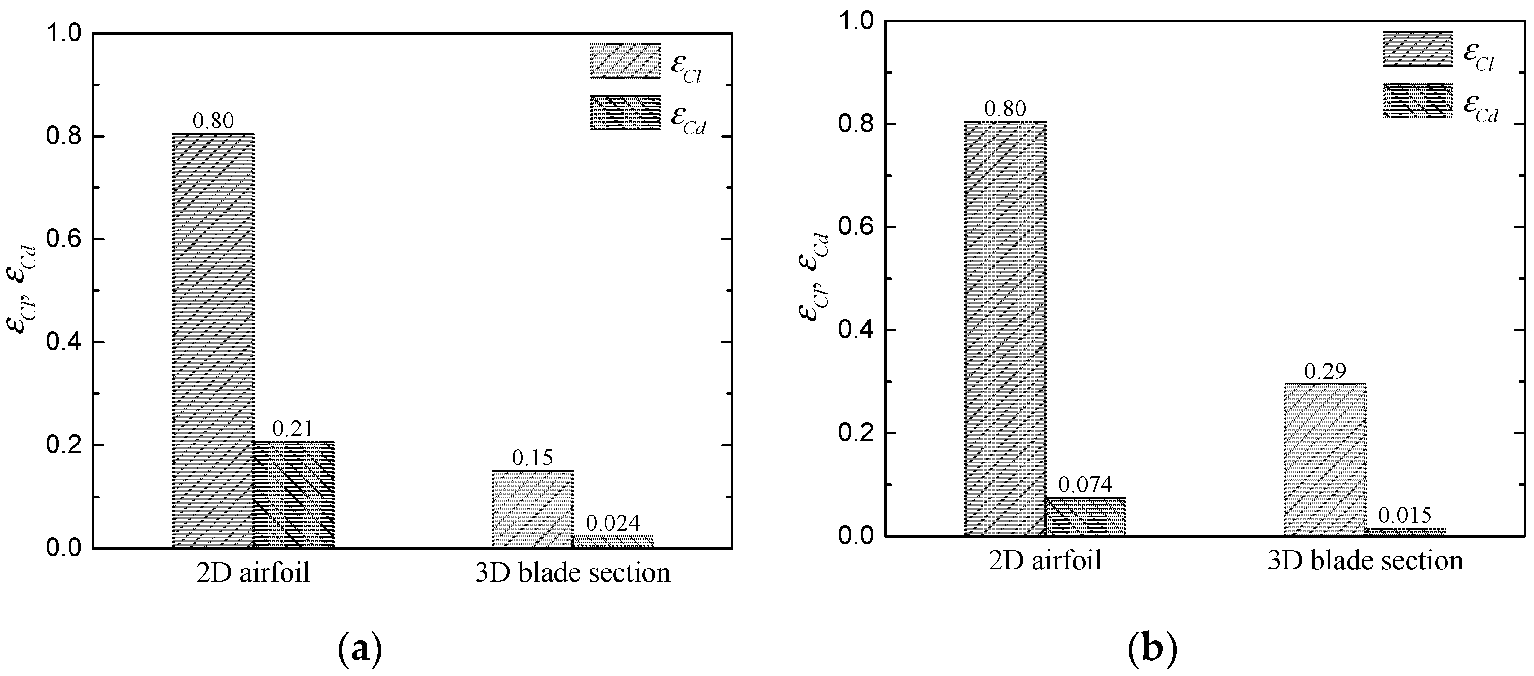
To quantify the combined effect on the lift and drag hysteresis intensities, we introduce the following parameters:
where A is the amplitude of AOA variation. εCl and εCd are determined over a complete cycle. Figure 10 illustrates that the percentage decreases of εCl and εCd have reached 60% and 80%, respectively. This finding demonstrates that rotational augmentation plays a key role in both the steady and unsteady aerodynamics of HAWTs. Increasing the wind speed can slightly attenuate the decrease in aerodynamic hysteresis, likely because the higher wind speed leads to the lower reduced frequency, i.e., the lower unsteadiness.
It should be noticed that dynamic stall plays a key role in the stall onset of blade flow and airfoil flow as well. Over the increasing AOA process, the unsteady Cl exceeds the static stall lift coefficient generally in the sense of extrapolating linear regime (Figure 8 and Figure 9). Therefore, the dynamic stall AOA and the dynamic stall Cl are further increased compared to the static stall values. We introduce the following parameters to determine the stall-delay amount with respect to stall Cl and stall AOA:
where and are the 2D static stall Cl and stall AOA. Figure 11 indicates that rotational augmentation and dynamics stall can separately and significantly delay the onset of stall. One can observe the higher ηCl and ηα due to dynamic stall than to rotational augmentation. This implies that dynamic stall is slightly stronger in delaying the onset of stall. Nevertheless, the increased ηCl and ηα of 3D unsteady flow indicate a further delayed stall compared to the 3D steady data, and the contribution of rotational augmentation becomes more significant.
5.2. Azimuthal Variation of the Pressure Distributions and Vorticity Field
To provide a deeper understanding of the complex unsteady flow mechanisms around the 3D blade section, we further analyze the unsteady pressure distributions to obtain an insight into the development of flow fields. As shown in Figure 2b and Figure 4a, the local AOA distribution is almost symmetrical around ϕa = 180°. This means that the local AOA is increasing on the upwind side of rotor plane, but decreasing on the downwind side. Figure 12 shows the upwind-side azimuthal variation of Cp distributions on the 3D blade section and 2D airfoil, and Figure 13 illustrates the associated flow development around 2D airfoil. Figure 14 and Figure 15 gives the downwind-side counterparts. The gray bars in Figure 12 and Figure 14 indicate the cycle-to-cycle variations of measured pressure. The great unsteadiness mainly appears on the retreating side of rotor plane due to the high AOA. One can observe that 2D pressure-side Cp distributions from ϕa = 30° to ϕa = 120° generally well agree with the 3D values (Figure 12). Based on the assumption that pressure-side Cp distributions of 3D blade section and 2D airfoil subject to the same AOA and do not change significantly in attached flow [29,30], this finding also demonstrates that present numerical modelling of 2D airfoil flow is sufficiently reliable.
Over the increasing AOA process, the 2D airfoil flow begins with a trailing-edge (T.E.) separated flow and the separation point remains around the mid-chord until ϕa = 90° (Figure 12 and Figure 13). Afterwards, the separation point jumps forward to the leading edge with the separation bubble bursting into small vortices and then alternately shedding into the wake. In contrast, the 3D blade flow begins with a fully attached flow. A short leading-edge (L.E.) separation occurs at ϕa = 60°, and then the separated zone extends to mid-chord with the local AOA increasing to ϕa = 150°. Adverse pressure gradients can be clearly observed between x/c = 0.36 and the trailing edge on the suction side, although the L.E. suction peak gradually decreases due to the extension of L.E. separation bubble. This implies that 3D blade flow is well attached aft of the reattachment point of L.E. separation, whereas the 2D airfoil flow falls into a long T.E. separation. Nevertheless, interesting to note is that the 2D Cl and 3D Cl are identical at ϕa = 150°, because the vortex lift of 2D airfoil flow effectively compensates the L.E. suction loss (Figure 12e).
Over the decreasing AOA process, the 2D airfoil flow remains in the state of vortex shedding until ϕa = 300° (Figure 14 and Figure 15). The onset of flow reattachment is substantially delayed, and hence the aerodynamic loads experience great hysteresis. In contrast, the L.E. separation bubble of 3D blade flow is effectively suppressed, and the flow field is almost fully reattached at ϕa = 270°, manifesting the rotational effects. Therefore, the 3D Cl is generally higher than the 2D Cl.
The comparative analysis of azimuthal variation of Cp distributions on the blade section and airfoil demonstrates a great difference in the flow mechanisms. The combined effect of rotational augmentation and dynamic stall is found to significantly suppress the separated flow in the manner of changing the massive T.E. separated flow into the moderate L.E. separated flow, avoid the separation bubble bursting, accelerate the flow reattachment over the decreasing AOA process, and eventually, reduce the aerodynamic hysteresis.
Gonzalez and Munduate [24] compared the Cp distributions of 2D airfoil and rotating blade section under axial inflow conditions, and they found that rotational augmentation on the NREL Phase VI rotor results from the suppressed growth of L.E. separated zone rather than the postponed forward movement of the T.E. separation point. This study indicates a similar effect of rotational augmentation under yawed inflow conditions. Bak et al. [23] proposed a rotational augmentation model based on the pressure-distribution difference between blade section and airfoil without yaw. Present comparative analysis suggests that the pressure-distribution difference with yaw is, however, highly complicated due to the vortex shedding around 2D airfoil. This means that a wide gap exists between the 2D airfoil flow and 3D blade flow, so that the yaw aerodynamics of blades should be directly modelled based on the deep understanding of 3D blade flow rather than correcting the existing 2D unsteady models or rudely combining the 2D dynamic stall models with the rotational augmentation models.
5.3. Dynamic Stall Regimes
From the Cp distributions, we further pinpoint where the flow separation and reattachment points are approximately located to analyze the dynamic stall regimes of blade section and airfoil. Figure 16 illustrates the different characteristics of separated flow around blade section and airfoil. For the 3D blade flow, distinct Cp plateaus indicate the presence of separation bubbles like A-B and C-D, which are originated at the leading and trailing edges separately. B-C shows a rapid increase in pressure, mainly because the transition leads to turbulent flow reattachment and makes the flow attached [24]. For the 2D airfoil, the Cp distribution indicates a long T.E. separated zone between the point b and point c, although a-b implies a high L.E. suction peak. In brief, point B denotes the reattachment point of L.E. separated flow on blade section, point C the T.E. separation point on blade section, and point b the T.E. separation point on airfoil. Then, the variation of separation and reattachment points with the local AOA can be obtained, as shown in Figure 17 and Figure 18.
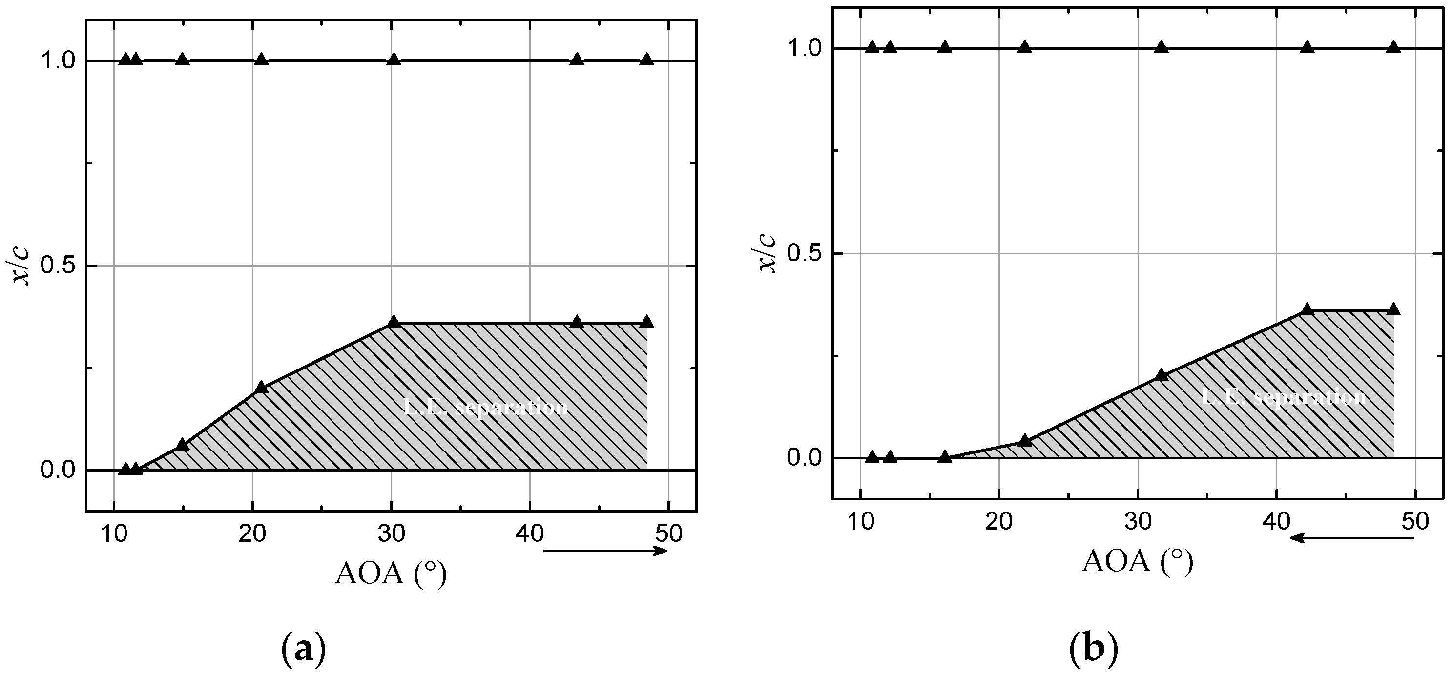
In general, Figure 17a,b and Figure 18a,b indicate the 3D blade flow to fall into the L.E. separation over one cycle. One can observe that the separated zone is wider over the increasing AOA process than over the decreasing AOA process. This manifests the rotational effects of accelerating the flow reattachment over the decreasing AOA process. In contrast, the 2D airfoil flow generally falls into the T.E. separation (Figure 17c,d and Figure 18c,d). The separated zone is narrower over the increasing AOA process than over the decreasing AOA process, implying that the rearward movement of T.E. separation point is well slower over the decreasing AOA process.
Guntur and Sørensen [25] compared the 3D blade flow and 2D airfoil flow of the MEXICO rotor, and they concluded that the rotational augmentation on this rotor results from the suppression of T.E. separated vortex in its thickness and length. The rotational augmentation around the NREL Phase VI blade, however, has indicated complex flow mechanisms even under the axial inflow conditions [24], although the NREL S809 airfoil is well known to fall into the same T.E. stall type [26,28]. This may cause a challenge of aerodynamic modelling in generality.
In the Beddoes-Leishman type dynamic stall models [38,39,42], the nonlinear forces are mainly determined by the so-called Kirchhoff flow model, based on the assumption that most airfoils fall into the progressive T.E. stall type. Additionally, a first-order lag to the separation point is often used to represent the effect of unsteady boundary layer responses [38]. This treatment is suitable for most of the 2D airfoil flow, and can lead to the slowed rearward movement of T.E. separation point over the decreasing AOA process, as shown in Figure 17 and Figure 18. In this study, we have found that the combined effect of rotational augmentation and dynamic stall may change the dynamic stall type from T.E. stall to L.E. stall, and bring about an opposite trend of the separated zone development in comparison with the 2D flow characteristics. These two key elements should be properly considered in the modelling of 3D unsteady blade flow so that the unsteady aerodynamic loads could be predicted accurately.
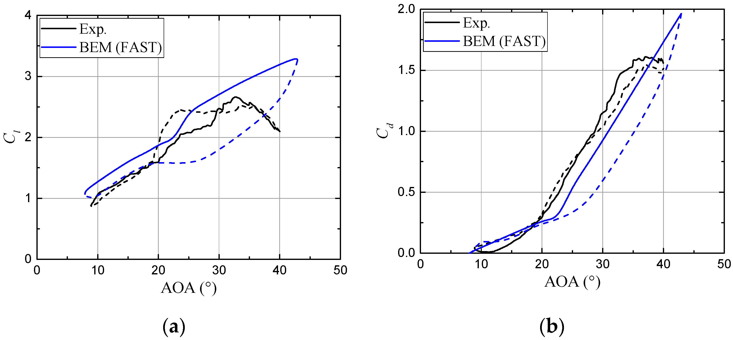
Figure 19 demonstrates a great discrepancy between the experimental and calculated aerodynamic coefficients, although both the rotational augmentation model and the dynamic stall model have been used in the FAST V8 [16,17]. In this BEM code, the Selig-Du model is applied to correct the 2D airfoil data firstly, and secondly, the Beddoes-Leishman model is used to further consider the unsteady effects of local AOA variations. The slightly wider AOA variation of BEM results can be ascribed to the larger amplitude of aerodynamic forces than the experimental data. Although the predicted 3D unsteady loads indicate the lower hysteresis intensities compared with the 2D unsteady loads (Figure 8c,d), the calculated hysteresis loops generally exhibit the main characteristics of 2D unsteady airfoil flow with respect to greatly retarded flow reattachment over the AOA decreasing process. This suggests a clear need for much more fundamental research into the flow mechanisms and the improved modelling with the coupled effect of rotational augmentation and dynamic stall included.
6. Conclusions
This paper presents a comprehensive comparative study between the 2D airfoil flow and 3D blade flow to provide a deep understanding of the combined effect of rotational augmentation and dynamic stall under yawed inflow conditions. The data of 3D blade flow directly come from the wind tunnel tests of the NREL Phase VI rotor, and the associated data of 2D unsteady airfoil flow are obtained by the URANS method. Present numerical modelling has been validated against the AMT theoretical results and the 3D experimental data of mid-blade where the 3D effects are negligible. This work aims to clarify the unsteady flow characteristics with and without rotational augmentation.
To obtain an insight into the flow mechanisms, we have analyzed the data in three aspects: aerodynamic hysteresis, flow field development, and dynamic stall regimes. The main finding about the combined effect of rotational augmentation and dynamic stall can be summarized in two aspects. First, the combined effect can favorably accelerate the flow reattachment over the decreasing AOA process and hence reduce the aerodynamic hysteresis. Second, it can significantly suppress the separated flow in the manner of changing the massive T.E. separated flow into the moderate L.E. separated flow, avoid the separation bubble bursting, and hence further delay the onset of stall. In addition, the 2D and 3D dynamic stall regimes imply a great difference in the separated zone development and stall type as well. Since a wide gap exists between the 2D airfoil flow and 3D blade flow, the aerodynamic modelling of rotating blades should not be made on basis of combining the existing 2D dynamic stall models and rotational augmentation correction models, but rather the deep understanding of 3D unsteady blade flow.
The major limitation of our study might be the limited experimental data about the 3D blade flow field. This may be resolved by means of CFD simulations whose overall predictive accuracy has to be validated at first. Nevertheless, this work can contribute to understanding and modelling the combined effect of rotational augmentation and dynamic stall on HAWTs.
Author Contributions
C.Z. conceived of the research, conducted the data collection and wrote the manuscript. T.W. and W.Z. contributed technical guidance and revised the manuscript.
Funding
This work is funded by the National Basic Research Program of China (973 Program) under grant No. 2014CB046200, CAS Key Laboratory of Wind Energy Utilization under grant No. KLWEU-2016-0102, and the Priority Academic Program Development of Jiangsu Higher Education Institutions.
Acknowledgments
The authors would like to express their gratitude to Lee Jay Fingersh of National Renewable Energy Laboratory (NREL) for providing the experimental data.
Conflicts of Interest
The authors declare no conflict of interest.
References
- Schepers, J.G. Engineering Models in Wind Energy Aerodynamics: Development, Implementation and Analysis Using Dedicated Aerodynamic Measurements; Delft University of Technology: Delft, The Netherlands, 2012. [Google Scholar]
- Schepers, J.G.; Boorsma, K.; Cho, T.; Gomez-Iradi, S.; Schaffarczyk, A.; Madsen, H.A.; Sorensen, N.N.; Shen, W.Z.; Lutz, T.; Sant, T.; et al. Final Report of IEA Wind Task 29: Mexnext (Phase 2); Energy Research Centre of The Netherlands: Petten, The Netherlands, 2014. [Google Scholar]
- Leishman, J.G. Challenges in modelling the unsteady aerodynamics of wind turbines. Wind Energy 2002, 5, 85–132. [Google Scholar] [CrossRef] [Green Version]
- Elgammi, M.; Sant, T. Combining unsteady blade pressure measurements and a free-wake vortex model to investigate the cycle-to-cycle variations in wind turbine aerodynamic blade loads in yaw. Energies 2016, 9, 27. [Google Scholar] [CrossRef]
- Leishman, J.G. Principles of Helicopter Aerodynamics, 2nd ed.; Cambridge University Press: Cambridge, UK, 2006. [Google Scholar]
- Johansen, J. Unsteady Airfoil Flows with Application to Aeroelastic Stability; Risø National laboratory: Roskilde, Denmark, 1999. [Google Scholar]
- McCroskey, W.J. The Phenomenon of Dynamic Stall; National Aeronautics and Space Administration: Washington, DC, USA, 1981. [Google Scholar]
- Carr, L.W. Progress in analysis and prediction of dynamic stall. J. Aircr. 1988, 25, 6–17. [Google Scholar] [CrossRef]
- Snel, H.; Houwink, R.; Bosschers, J. Sectional Prediction of LIft Coefficients on Rotating Wind Turbine Blades in Stall; Energy Research Center of The Netherlands: Petten, The Netherlands, 1993. [Google Scholar]
- Du, Z.; Selig, M. A 3-D stall-delay model for horizontal axis wind turbine performance prediction. In Proceedings of the 36th AIAA Aerospace Sciences Meeting and Exhibit, ASME Wind Energy Symposium, Reno, NV, USA, 12–15 January1998. [Google Scholar]
- Schreck, S.; Robinson, M. Rotational augmentation of horizontal axis wind turbine blade aerodynamic response. Wind Energy 2002, 5, 133–150. [Google Scholar] [CrossRef]
- Lindenburg, C. Investigation into Rotor Blade Aerodynamics; Energy Research Centre of The Netherlands: Petten, The Netherlands, 2003. [Google Scholar]
- Bangga, G. Three-Dimensional Flow in the Root Region of Wind Turbine Rotors; Kassel University Press: Kassel, Germany, 2018. [Google Scholar]
- Breton, S.P.; Coton, F.N.; Moe, G. A Study on rotational effects and different stall delay models using i a prescribed wake vortex scheme and NREL phase VI experiment data. Wind Energy 2008, 11, 459–482. [Google Scholar] [CrossRef]
- Larsen, J.W.; Nielsen, S.R.K.; Krenk, S. Dynamic stall model for wind turbine airfoils. J. Fluids Struct. 2007, 23, 959–982. [Google Scholar] [CrossRef]
- Jonkman, B.; Jonkman, J. FAST v8.16.00a-bjj; National Renewable Energy Laboratory: Golden, CO, USA, 2016.
- Damiani, R.; Hayman, G. The Dynamic Stall Module for FAST 8; National Renewable Energy Laboratory: Golden, CO, USA, 2016.
- Duque, E.P.N.; Burklund, M.D.; Johnson, W. Navier-stokes and comprehensive analysis performance predictions of the NREL phase VI experiment. J. Sol. Energy Eng. 2003, 125, 457–467. [Google Scholar] [CrossRef]
- Schepers, J.G. IEA Annex XX: Comparison between Calculations and Measurements on a Wind Turbine in Yaw in the NASA-Ames Wind Tunnel; Energy Research Center of The Netherlands: Petten, The Netherlands, 2007. [Google Scholar]
- Tongchitpakdee, C.; Benjanirat, S.; Sankar, L.N. Numerical simulation of the aerodynamics of horizontal axis wind turbines under yawed flow conditions. In Proceedings of the 43rd AIAA Aerospace Sciences Meeting and Exhibit, Reno, NV, USA, 10–13 January 2005; pp. 14015–14025. [Google Scholar]
- Yu, D.O.; You, J.Y.; Kwon, O.J. Numerical investigation of unsteady aerodynamics of a Horizontal-axis wind turbine under yawed flow conditions. Wind Energy 2013, 16, 711–727. [Google Scholar] [CrossRef]
- Schreck, S.; Robinson, M. Dynamic stall and rotational augmentation in recent wind turbine aerodynamics experiments. In Proceedings of the 32nd AIAA Fluid Dynamics Conference and Exhibit, St. Louis, MO, USA, 24–26 June 2002. [Google Scholar]
- Bak, C.; Johansen, J.; Andersen, P.B. Three-dimensional corrections of airfoil characteristics based on pressure distributions. In Proceedings of the European Wind Energy Conference and Exhibition (EWEC), Athens, Greece, 27 February–2 March 2006. [Google Scholar]
- Gonzalez, A.; Munduate, X. Three-dimensional and rotational aerodynamics on the NREL Phase VI wind turbine blade. In Proceedings of the 45th AIAA Aerospace Sciences Meeting, Reno, NV, USA, 8–11 January 2007; pp. 7597–7610. [Google Scholar]
- Guntur, S.; Sorensen, N.N. A study on rotational augmentation using CFD analysis of flow in the inboard region of the MEXICO rotor blades. Wind Energy 2015, 18, 745–756. [Google Scholar] [CrossRef]
- Ramsay, R.F.; Hoffman, M.J.; Gregorek, G.M. Effects of Grit Roughness and Pitch Oscillation on the S809 Airfoil; National Renewable Energy Laboratory: Golden, CO, USA, 1995.
- Hand, M.M.; Simms, D.A.; Fingersh, L.J.; Jager, D.W.; Cotrell, J.R.; Schreck, S.J.; Larwood, S.M. Unsteady Aerodynamics Experiment Phase VI: Wind Tunnel Test. Configurations and Available Data Campaigns; National Renewable Energy Laboratory: Golden, CO, USA, 2001.
- Somers, D.M. Design and Experimental Results for the S809 Airfoil; National Renewable Energy Laboratory: Golden, CO, USA, 1997. [Google Scholar]
- Shipley, D.E.; Miller, M.S.; Robinson, M.C.; Luttges, M.W.; Simms, D.A. Techniques for the Determination of Local Dynamic Pressure and Angle of Attack on a Horizontal Axis Wind Turbine; National Renewable Energy Laboratory: Golden, CO, USA, 1995.
- Guntur, S.; Sørensen, N.N. An evaluation of several methods of determining the local angle of attack on wind turbine blades. In Proceedings of the Science of Making Torque from Wind, Oldenburg, Germany, 9–11 October 2012; Volume 555. [Google Scholar]
- Hansen, M.O.L. Aerodynamics of Wind Turbines, 2nd ed.; Earthscan: London, UK, 2008. [Google Scholar]
- ANSYS Inc. FLUENT. Theory Guide, Release 16.0; ANSYS Inc. FLUENT: Canonsburg, PA, USA, 2015. [Google Scholar]
- Zhu, C.; Wang, T. Comparative study of dynamic stall under pitch oscillation and oscillating freestream on wind turbine airfoil and blade. Appl. Sci. 2018, 8, 1242. [Google Scholar] [CrossRef]
- Zhu, C.; Wang, T.; Wu, J. Numerical investigation of passive vortex generators on a wind turbine airfoil undergoing pitch oscillations. Energies 2019, 12, 654. [Google Scholar] [CrossRef]
- Menter, F.R. Two-equation eddy-viscosity transport turbulence model for engineering applications. AIAA J. 1994, 32, 1598–1605. [Google Scholar] [CrossRef]
- Menter, F.R.; Langtry, R.B.; Likki, S.R.; Suzen, Y.B.; Huang, P.G.; Volker, S. A correlation-based transition model using local variables—Part I: Model formulation. J. Turbomach. Trans. ASME 2006, 128, 413–422. [Google Scholar] [CrossRef]
- Ekaterinaris, J.A.; Platzer, M.F. Computational prediction of airfoil dynamic stall. Prog. Aerosp. Sci. 1997, 33, 759–846. [Google Scholar] [CrossRef]
- Leishman, J.G.; Beddoes, T.S. A semi-empirical model for dynamic stall. J. Am. Helicopter Soc. 1989, 34, 3–17. [Google Scholar] [CrossRef]
- Hansen, M.H.; Gaunaa, M.; Madsen, H.A. A Beddoes-Leishman Type Dynamic Stall Model in State-Space and Indicial Formulation; Risø National Laboratory: Roskilde, Denmark, 2004. [Google Scholar]
- Van der Wall, B.G.; Leishman, J.G. On the influence of time-varying flow velocity on unsteady aerodynamics. J. Am. Helicopter Soc. 1994, 39, 25–36. [Google Scholar] [CrossRef]
- Sant, T.; van Kuik, G.; van Bussel, G.J.W. Estimating the angle of attack from blade pressure measurements on the national renewable energy laboratory phase VI rotor using a free wake vortex model: Yawed conditions. Wind Energy 2009, 12, 1–32. [Google Scholar] [CrossRef]
- Gupta, S.; Leishman, J.G. Dynamic stall modelling of the S809 aerofoil and comparison with experiments. Wind Energy 2006, 9, 521–547. [Google Scholar] [CrossRef]
Figure 1.
Schematic of comparative studies of aerodynamic characteristics between the wind turbine airfoil and blade section. ‘RA’ denotes rotational augmentation, ‘DS’ dynamic stall, and ‘RA+DS’ combined effect of rotational augmentation and dynamic stall.
Figure 1.
Schematic of comparative studies of aerodynamic characteristics between the wind turbine airfoil and blade section. ‘RA’ denotes rotational augmentation, ‘DS’ dynamic stall, and ‘RA+DS’ combined effect of rotational augmentation and dynamic stall.

Figure 2.
Schematic of a horizontal axis wind turbine under yawed inflow. (a) top view; (b) front view.
Figure 2.
Schematic of a horizontal axis wind turbine under yawed inflow. (a) top view; (b) front view.

Figure 3.
Schematic of the sectional velocity triangle and aerodynamic forces. (a) velocity triangle; (b) aerodynamic forces.
Figure 3.
Schematic of the sectional velocity triangle and aerodynamic forces. (a) velocity triangle; (b) aerodynamic forces.

Figure 4.
Azimuthal variations of the AOA and resultant velocity at 13 m/s wind speed and 30° yaw angle (S1300300). (a) AOA; (b) resultant velocity.
Figure 4.
Azimuthal variations of the AOA and resultant velocity at 13 m/s wind speed and 30° yaw angle (S1300300). (a) AOA; (b) resultant velocity.

Figure 5.
Hysteresis loops of the lift and drag coefficients in deep stall of the NREL S809 airfoil undergoing pitch oscillation. α = 20 ± 10°, k = 0.078, and Re = 1 × 10⁶. (a) Cl; (b) Cd.
Figure 5.
Hysteresis loops of the lift and drag coefficients in deep stall of the NREL S809 airfoil undergoing pitch oscillation. α = 20 ± 10°, k = 0.078, and Re = 1 × 10⁶. (a) Cl; (b) Cd.

Figure 6.
Unsteady lift coefficient of the NREL S809 airfoil at different amplitudes of velocity variation. Cl0 is the quasi-steady lift coefficient at V0. Solid lines denote the URANS results, and dashed lines the theoretical results.
Figure 6.
Unsteady lift coefficient of the NREL S809 airfoil at different amplitudes of velocity variation. Cl0 is the quasi-steady lift coefficient at V0. Solid lines denote the URANS results, and dashed lines the theoretical results.

Figure 7.
Unsteady pressure distributions of the 63% span on the NREL Phase VI rotor at different azimuths. Vw = 7 m/s and ϕy = 30° (S0700300). (a) ϕa = 0°; (b) ϕa = 90°; (c) ϕa = 180° (d) ϕa = 270°.
Figure 7.
Unsteady pressure distributions of the 63% span on the NREL Phase VI rotor at different azimuths. Vw = 7 m/s and ϕy = 30° (S0700300). (a) ϕa = 0°; (b) ϕa = 90°; (c) ϕa = 180° (d) ϕa = 270°.

Figure 8.
Hysteresis loops of the lift and drag coefficients. r/R = 30%, Vw = 13 m/s, and ϕy = 30°. Solid lines denote increasing AOA, and dashed lines decreasing AOA. (a) 3D Cl; (b) 3D Cd; (c) 2D Cl; (d) 2D Cd.
Figure 8.
Hysteresis loops of the lift and drag coefficients. r/R = 30%, Vw = 13 m/s, and ϕy = 30°. Solid lines denote increasing AOA, and dashed lines decreasing AOA. (a) 3D Cl; (b) 3D Cd; (c) 2D Cl; (d) 2D Cd.

Figure 9.
Hysteresis loops of the lift and drag coefficients. r/R = 30%, Vw = 15 m/s, and ϕy = 30°. Solid lines denote increasing AOA, and dashed lines decreasing AOA. (a) 3D Cl; (b) 3D Cd; (c) 2D Cl; (d) 2D Cd.
Figure 9.
Hysteresis loops of the lift and drag coefficients. r/R = 30%, Vw = 15 m/s, and ϕy = 30°. Solid lines denote increasing AOA, and dashed lines decreasing AOA. (a) 3D Cl; (b) 3D Cd; (c) 2D Cl; (d) 2D Cd.

Figure 10.
Lift and drag hysteresis intensities of the 2D airfoil and 3D blade section. (a) Vw = 13 m/s; (b) Vw = 15 m/s.
Figure 10.
Lift and drag hysteresis intensities of the 2D airfoil and 3D blade section. (a) Vw = 13 m/s; (b) Vw = 15 m/s.

Figure 11.
Stall-delay parameters of the 2D airfoil and 3D blade section. ‘RA’ denotes rotational augmentation, ‘DS’ dynamic stall, and ‘RA + DS’ combined effect of rotational augmentation and dynamic stall. Blue bars denote the unsteady effects on 3D blade flow. (a) Vw = 13 m/s; (b) Vw = 15 m/s.
Figure 11.
Stall-delay parameters of the 2D airfoil and 3D blade section. ‘RA’ denotes rotational augmentation, ‘DS’ dynamic stall, and ‘RA + DS’ combined effect of rotational augmentation and dynamic stall. Blue bars denote the unsteady effects on 3D blade flow. (a) Vw = 13 m/s; (b) Vw = 15 m/s.

Figure 12.
Azimuthal variation of the pressure distributions on the upwind side of rotor plane. r/R = 30%, Vw = 15 m/s, and ϕy = 30°. 3D data are mean ± SD. (a) ϕa = 30°; (b) ϕa = 60°; (c) ϕa = 90° (d) ϕa = 120°; (e) ϕa = 150°.
Figure 12.
Azimuthal variation of the pressure distributions on the upwind side of rotor plane. r/R = 30%, Vw = 15 m/s, and ϕy = 30°. 3D data are mean ± SD. (a) ϕa = 30°; (b) ϕa = 60°; (c) ϕa = 90° (d) ϕa = 120°; (e) ϕa = 150°.

Figure 13.
Development of the vorticity field around the 2D airfoil from ϕa = 30° to ϕa = 150°.

Figure 14.
Azimuthal variation of the pressure distributions on the downwind side of rotor plane. r/R = 30%, Vw = 15 m/s, and ϕy = 30°. 3D data are mean ± SD. (a) ϕa = 210°; (b) ϕa = 240°; (c) ϕa = 270° (d) ϕa = 300°; (e) ϕa = 330°.
Figure 14.
Azimuthal variation of the pressure distributions on the downwind side of rotor plane. r/R = 30%, Vw = 15 m/s, and ϕy = 30°. 3D data are mean ± SD. (a) ϕa = 210°; (b) ϕa = 240°; (c) ϕa = 270° (d) ϕa = 300°; (e) ϕa = 330°.

Figure 15.
Development of the vorticity field around the 2D airfoil from ϕa = 210° to ϕa = 330°.

Figure 16.
Pressure distributions of the 3D blade section and 2D airfoil at ϕa = 90°. r/R = 30%, Vw = 13 m/s, and ϕy = 30°.
Figure 16.
Pressure distributions of the 3D blade section and 2D airfoil at ϕa = 90°. r/R = 30%, Vw = 13 m/s, and ϕy = 30°.

Figure 17.
Comparison of flow separation and reattachment between the blade section and airfoil. r/R = 30%, Vw = 13 m/s, and ϕy = 30°. (a) 3D blade flow with increasing AOA; (b) 3D blade flow with decreasing AOA; (c) 2D airfoil flow with increasing AOA; (d) 2D airfoil flow with decreasing AOA.
Figure 17.
Comparison of flow separation and reattachment between the blade section and airfoil. r/R = 30%, Vw = 13 m/s, and ϕy = 30°. (a) 3D blade flow with increasing AOA; (b) 3D blade flow with decreasing AOA; (c) 2D airfoil flow with increasing AOA; (d) 2D airfoil flow with decreasing AOA.

Figure 18.
Comparison of flow separation and reattachment between the blade section and airfoil. r/R = 30%, Vw = 15 m/s, and ϕy = 30°. (a) 3D blade flow with increasing AOA; (b) 3D blade flow with decreasing AOA; (c) 2D airfoil flow with increasing AOA; (d) 2D airfoil flow with decreasing AOA.
Figure 18.
Comparison of flow separation and reattachment between the blade section and airfoil. r/R = 30%, Vw = 15 m/s, and ϕy = 30°. (a) 3D blade flow with increasing AOA; (b) 3D blade flow with decreasing AOA; (c) 2D airfoil flow with increasing AOA; (d) 2D airfoil flow with decreasing AOA.


Figure 19.
Comparison between the experimental aerodynamic coefficients and the calculated data with both rotational augmentation and dynamic stall models used in the BEM code. r/R = 30%, Vw = 13 m/s, and ϕy = 30°. Solid lines denote increasing AOA, and dashed lines decreasing AOA. (a) 3D Cl; (b) 3D Cd.

© 2019 by the authors. Licensee MDPI, Basel, Switzerland. This article is an open access article distributed under the terms and conditions of the Creative Commons Attribution (CC BY) license (http://creativecommons.org/licenses/by/4.0/).
Share and Cite
MDPI and ACS Style
Zhu, C.; Wang, T.; Zhong, W. Combined Effect of Rotational Augmentation and Dynamic Stall on a Horizontal Axis Wind Turbine. Energies 2019, 12, 1434. https://doi.org/10.3390/en12081434
AMA Style
Zhu C, Wang T, Zhong W. Combined Effect of Rotational Augmentation and Dynamic Stall on a Horizontal Axis Wind Turbine. Energies. 2019; 12(8):1434. https://doi.org/10.3390/en12081434
Chicago/Turabian StyleZhu, Chengyong, Tongguang Wang, and Wei Zhong. 2019. "Combined Effect of Rotational Augmentation and Dynamic Stall on a Horizontal Axis Wind Turbine" Energies 12, no. 8: 1434. https://doi.org/10.3390/en12081434
Note that from the first issue of 2016, this journal uses article numbers instead of page numbers. See further details here.