Wake Management in Wind Farms: An Adaptive Control Approach

Abstract

Advanced wind measuring systems like Light Detection and Ranging (LiDAR) is useful for wake management in wind farms. However, due to uncertainty in estimating the parameters involved, adaptive control of wake center is needed for a wind farm layout. LiDAR is used to track the wake center trajectory so as to perform wake control simulations, and the estimated effective wind speed is used to model wind farms in the form of transfer functions. A wake management strategy is proposed for multi-wind turbine system where the effect of upstream turbines is modeled in form of effective wind speed deficit on a downstream wind turbine. The uncertainties in the wake center model are handled by an adaptive PI controller which steers wake center to desired value. Yaw angle of upstream wind turbines is varied in order to redirect the wake and several performance parameters such as effective wind speed, velocity deficit and effective turbulence are evaluated for an effective assessment of the approach. The major contributions of this manuscript include transfer function based methodology where the wake center is estimated and controlled using LiDAR simulations at the downwind turbine and are validated for a 2-turbine and 5-turbine wind farm layouts.

1. Introduction

Wind power installations require precise control throughout their lifetime for optimal power generation with minimal risk of loss of security and reliability. Wind turbines placed in a particular fashion in a wind farm often experience low power production and high turbulence owing to wake effects from upwind turbines. Wind wakes lead to low power production, reduce system efficiency and necessitate appropriate control action for the entire wind farm. Wake effects from adjacent wind turbines termed as wake mixing lead to change in ambient wind field conditions that alter dynamic loading on the downwind turbines [1]. Wake models with varying fidelity have been developed over the years with Jensen’s and Frandsen’s model being used widely for calculating velocity deficit for a given downwind turbine. Additionally, added turbulence to the ambient wind field is a significant cause for concern among wind farm operators.

Recently, a lot of focus has been laid on the control based dynamic models that modify wake characteristics for a particular downwind turbine. The main goals of wind turbine and wind farm control are to: (i) maximize power capture from the available wind resource and, (ii) minimize the structural loading caused by wake added turbulence [2]. The dynamic nature of wind causes power fluctuations which can lead to reserve power capacity in terms of Battery energy storage system (BESS). Efficient wind farm control can be achieved by two primary methods: (i) axial induction method that aims to alter the pitch angle every time wind speed changes and optimizes rotor angle to capture maximum power, and (ii) wake redirecting control which deflects the wake stream in order to achieve optimal power capture for downwind turbines in a wind farm [3].

Simulation studies as well as experimental results have revealed that changing yaw angle of the upwind turbine deflects the wake center of the wake field and changes the effective rotor area under the shadow of upwind turbine [4]. Apart from yaw angle modification for upwind turbine, repositioning of downwind turbines has been explored by Gebraad et al. [5]. In [6], Fleming et al. have discussed several methods like individual pitch control (IPC) and tilt induced control to redirect wake of wind field for the downstream turbines and various performance parameters are analyzed using a high fidelity tool Simulator for On/Offshore Wind Farm Applications (SOWFA). Adaramola et al. experimentally verified wake interference scenario where the total power capture from two wind turbines was found to increase by 12% by operating upwind turbine in yawed condition [7]. The impact of terrain and the effect of turbulent wind on power output was studied experimentally by Maeda et al. with two Horizontal axis wind turbines (HAWT) placed in a wind tunnel [8]. In terms of optimization, total power is optimized considering optimal induction factor and yaw angle control for a wind farm with a single column layout [9]. Closed-loop control was first studied by Raach et al. where the wake tracking characteristics are obtained through LiDAR mounted on wind turbine nacelle [10]. The wake center is estimated for a given downwind turbine and based on the estimation, the yaw angle of the upwind turbine is varied. Doubrawa et al. have carried out experimental studies on wind turbine wake characterization based on LiDAR measurements [11]. Results reveal that the wind speed measurements carried out using LES data are found to be in good approximation with those from LiDAR. Furthermore, on similar grounds, for wake characterization, a stochastic model is developed that traces the wake shape and width [12]. The developed model on LES framework holds true for far wake region thus removing limitations posed by Reynolds–averaged Navier Stokes (RANS) model. Wang et al. have discussed various errors in measurement of radial velocity variance based on doppler LiDAR [13]. Results indicate that LiDAR measurements nullify the errors in radial velocity variance that aids accurate measurement of turbulence. Furthermore, the length of probe affects the errors in radial velocity variance. A major challenge in addressing the control of wind farm is the availability of accurate and precise measurement devices that are essential for the controller to change the turbine properties.

Due to the uncertainties like the random wind and the unpredictable wake affect, the wind farms require highly efficient control schemes so as to achieve good performance. Adaptive control is a mechanism used when the system encounters uncertainties due to its ability to adapt or handle parameter uncertainties [14,15,16,17]. The parameter estimator estimates the unknown or uncertain parameter. Adaptive control provides automatic adjustment of controllers for maintaining desired system performance when system parameters are not precisely known [18,19,20,21]. The performance of the system is measured and compared with the desired values. Based on the error term generated by comparison, the adjustable controller adapts the changed condition through different adaption mechanisms. Such adaptive control techniques are also developed and further analysis has taken place.

The major contributions of this paper include transfer function based methodology where the wake center is estimated and controlled using LiDAR simulations at the downwind turbine. The wake management for a wind farm is achieved by controlling the wake center for desired yaw angle of wind turbine based on an adaptive control. The proposed methodology based on the effective velocity deficit and effective wake center is validated for multi-model wake scenario and multiple wake scenario for a 5-turbine wind farm layout.

This paper is organized as follows. Section 2 describes the closed-loop control methodology and Section 3 highlights the wake center formulation for multi-model and multiple wake scenario. In Section 4 various performance parameters are discussed for waked wind farms, and in Section 5, framework for test model and simulation results are illustrated for the wind farm performance.

2. Methodology

The closed-loop control strategy revolves around two basic tasks, that is: (i) estimation of wind field measurements and, (ii) control of the wake center position for desired yaw angle input. The LiDAR sensor works on the principle of laser based light assisted detection and ranging which measures the incoming wind speed from an upwind turbine placed at at a particular distance known as LiDAR distance ($d_{LiDAR}$). The yaw angle adjustment however decreases the power captured by the upwind turbine and increases the same for downwind turbine. Wake center on the other hand has no definition as per the recent literature involving the closed-loop control of the wind farm [22]. The current work deals with a wake management strategy based on transfer function model for wind turbine and wake center estimation. Furthermore, the wake center trajectory is tracked based on LiDAR simulations and is controlled for desired yaw angle of upstream turbines. The LiDAR is used to track the position of wake center in order to steer the wake flow away from downstream turbine. LiDAR gives an estimate of wind speed before it actually interacts with turbine thus providing necessary information to the adaptive controller to act in uncertain conditions. The wake center deflection due to yaw misalignment is further explained in Section 2.2.

LiDAR is Light Detection and Ranging system installed at the top of wind turbine nacelle for accurate wind speed measurement. The wind speed is measured before it interacts with the wind turbine thus ensuring time for effective control strategies for improved wind farm performance [23]. Two types of LiDAR measurement systems are commercially available: continuous-wave (CW) LiDAR and pulsed-wave LiDAR, but the former is preferred for economic reasons [24]. LiDAR emits a laser beam of specified frequency and wavelength and the receiver collects the backscattered beam for further processing. The LiDAR efficiency depends on the range for which the beam is used. The detected wind speed is then processed for Doppler spectra using Fourier analysis and then it is time-averaged followed by line-of-sight velocity estimation.

Next, we describe various components of closed-loop control of wake center estimation: wind turbine model, wake center estimation model and control action for desired yaw angle alignment. Figure 1 shows a schematic block diagram of wake center estimation based on an adaptive PI control strategy for a desired yaw angle.

2.1. Wind Turbine Model

The wind turbine is modeled from basic actuator disk theory with the extracted power from $i^{th}$ wind turbine wind given as

$$\begin{array}{c}\hfill P_i=\frac{1}{2}\rho A_0{C}_p{u}_i^3,\end{array}$$

(1)

where $\rho$ is the air density, $A_0$ is the swept rotor area, $C_p$ is the power coefficient and $u_i$ is the wind speed at the $i^{th}$ turbine [25]. However, in case of yawed wind turbines, the power output from the upwind turbine is altered by a factor of ${cos}^q\gamma$, where q is a tunable parameter. According to experimental studies carried out by Fleming et al., the wake steering is observed for $q=1.4$ to $q=2.2$ [26]. Furthermore, in a study carried out by Jonkman et al., it is found that the power coefficient of upstream turbine in yawed condition gets modified by a factor ${cos}^q\gamma$ [27]. In order to capture power at a maximum value of $C_p=0.482$ including losses accounted by turbulent wakes, the value of q is found to be 2. In this paper, we consider a 2-DOF model for a nacelle and the yaw alignment of an upwind turbine is modeled according to a 2^nd order differential equation given as

$$\begin{array}{c}\hfill \ddot{\gamma }+2D\omega \dot{\gamma }+{\omega }^2\gamma ={\omega }^2{\gamma }_{ref},\end{array}$$

(2)

where $\omega$ is the undamped eigen frequency, D is the damping factor, ${\gamma }_{ref}$ is the desired yaw angle input for the wind turbine.

The transfer function for the wind turbine is estimated using system identification toolbox with a reference yaw angle (${\gamma }_{ref}$) being the input and $\gamma$ being the actual yaw angle. The demanded yaw angle is varied from −25${}^{\circ }$ to 25${}^{\circ }$ and the recorded output $\gamma$ is calculated. The transfer function so obtained has estimation accuracy of 99.99% with $n_p=2$ poles and $n_z=1$ zero and is of the form

$$\begin{array}{c}\hfill G_1(s)=\frac{0.533s+0.01094}{s^2+0.1538s+0.002736}.\end{array}$$

(3)

Optimized power from an upstream wind turbine in yawed condition as stated by Qian et al. [28] is given as

$$\begin{array}{c}\hfill P_i=\frac{1}{2}\rho A_0{C}_p{u}_i^3{cos}^3({\gamma }_i).\end{array}$$

(4)

In (4), the power captured by an upstream turbine is calculated based on the yaw angle setting corrected by the adaptive PI controller. LiDAR simulations track the wake center in order to steer it to a desired value. The wind turbine model is based on the yaw misalignment of the turbine which further impacts the power captured at the downstream turbine by deflecting the wake flow behind upstream turbine. The velocity profile at the downstream turbine is further explained in Section 4. In totality, the wind turbine model based on yaw misalignment forms an integral part of the wake management strategy.

2.2. Wake Center Estimation

Various closed-loop control studies done for wind farm power improvement involve estimation of center of the wake field originating from the upwind turbine. The wake center position for a given upwind turbine can be estimated using several functional relationships between the yaw angle misalignment and longitudinal distance between the turbines. Howland et al. have demonstrated the estimation error between experimental and theoretical wake center deflection is found to be $\pm 0.02D$ for a 3D printed porus drag disk model of wind turbine [4]. Empirically, wake center is calculated for a yawed upwind turbine and depends on the downwind distance d between two turbines. As per Jimnez et al. [29], the wake center due to yaw misalignment is given as

$$\begin{array}{ccc}\hfill \delta (d)& =& \frac{{\xi }_{init}\left(15{\left(\frac{2k_{d}d}{D_0}+1\right)}^4+{\xi }_{init}^2\right)}{\frac{30k_d}{D_0}{\left(\frac{2k_{d}d}{D_0}+1\right)}^5}-\frac{{\xi }_{init}{D}_0(15+{\xi }_{init}^2)}{30k_d},\hfill \end{array}$$

(5)

$$\begin{array}{ccc}\hfill {\xi }_{init}(\gamma ,C_T)& =& \frac{1}{2}{cos}^2(\gamma )sin(\gamma )C_T,\hfill \end{array}$$

(6)

$$\begin{array}{ccc}\hfill M_{\gamma }& =& -2\dot{\gamma }\Omega cos\psi I_b,\hfill \end{array}$$

(7)

where ${\xi }_{init}$ is the initial angle the wake stream makes with rotor axis of the upwind turbine, d is the distance between upwind and downwind turbine, $D_0$ is the turbine diameter, $\gamma$ is the yaw angle of the upwind turbine and $k_d$ is the model parameter subjected to uncertainties. Furthermore, Equation (7) represents the yaw bearing moment due to yaw misalignment where $\dot{\gamma }$ is the yaw rate (in rad/sec), $\Omega$ is the angular velocity of rotor, $\psi$ is the azimuth angle of blades and $I_b$ is the moment of inertia of blades [30].

The most challenging problem in modeling the wake effects is the tuning of model parameter $k_d$ which defines the wake recovery. The LiDAR based closed-loop control method scans various points in wind field located at a particular distance and measures the effective wind speed at the rotor hub [31]. In order to compute the wake center deflection caused due to changing yaw angles, appropriate LiDAR distance $d_{LiDAR}$ must be considered for accurate wake center estimation. The transfer function for the wake center estimation is computed using the system identification toolbox available in MATLAB/Simulink and is estimated for single set of upwind and downwind turbine. The yaw angle that needs to be aligned, acts as the input and estimated the wake center acts as the output of the transfer function. The values of yaw angle (in degrees) are varied in the range of −25${}^{\circ }$ to 25${}^{\circ }$ and the corresponding values of wake center are obtained using (5). The model parameter $k_d$ is chosen as 0.15 and is subjected to variations under different atmospheric conditions. The transfer function for the wake estimation model obtained with estimation accuracy of 93.76% with $n_p=2$ poles and $n_z=0$ zeros and is of form

$$\begin{array}{c}\hfill G_2(s)=\frac{-0.158}{s^2+2.56\times {10}^{-12}s+0.2404}.\end{array}$$

(8)

2.3. Controller Design

The main aspect of the wake center estimation process is its control for desired yaw angle alignment in order to maximize wind power capture for the downwind turbines. A simple PI control based strategy is applied in order to maximize wind farm performance in terms of power capture, effective turbulence, velocity deficit and turbine tower displacement. A PI control of the following form is selected to achieve desired performance

$$\begin{array}{c}\hfill f=K_p\left(\delta (\gamma )+\frac{1}{T_i}\int \delta (\gamma )dt\right),\end{array}$$

(9)

where f is the yaw angle for the turbine, $\delta (\gamma )$ is the estimated wake center, $K_p,T_i$ are the proportional gain and time constant. The PI control gain parameters are tuned using PID tuning feature of MATLAB/Simulink.

3. Wake Center Estimation and Adaptive Control

LiDAR based wake center estimation and control can be further extended for a multi-model approach where a single set of upwind and downwind turbine is evaluated for different input conditions. The wake center estimation depends on several factors like initial wake stream angle, distance between upwind and downwind turbine, rotor diameter and model parameter $k_d$ as defined in (5). Furthermore, apart from aforementioned factors the wake development zone, that is, near-wake zone and far-wake zone also plays an important role in estimating the wake center [32]. In the present study the multi-model wake center estimation is studied using a data-driven approach where the model parameter $k_d$ is kept constant and the LiDAR scanning distance, that is, $d_{LiDAR}$ is varied in terms of multiples of rotor diameter ($D_0$). Figure 2 shows a diagrammatic representation for multi-model transfer function-based estimation of wake center. The control objective is to track a reference wake center for yaw angle alignment of upwind turbine in a given wind farm in presence of uncertainties. Several transfer function models can be obtained by varying LiDAR scanning distance ($d_{LiDAR}$). The conventional PID control method can be expanded by using an adaptive PI controller for different models of wake center estimation. The transfer function for the respective models can be obtained using System identification toolbox available in MATLAB/Simulink and its estimation accuracies are depicted in

Table 1. Estimationaccuracies for multi-model transfer function models.

LiDAR Distance (${\mathit{d}}_{\mathit{LiDAR}}$)	Estimation Accuracy (%)
$1D_0$	93.76
$1.5D_0$	95.08
$2D_0$	94.94
$2.5D_0$	94.82
$3D_0$	94.71

.

Wake Center Estimation and Control for Multiple Turbines

In the previous section, we study the wake center estimation and control for a single set of upwind and downwind turbine. However, in reality there are multiple upwind turbines for a given downwind turbine in a wind farm layout. The wake trajectory for a downwind turbine depends on the layout of the wind farm which may be symmetrical or asymmetrical. For multiple upwind turbines, the effective velocity deficit can be estimated based on wake model proposed by Bastankhah and Porte-Agel [33]. The model assumes a Gaussian profile for velocity deficit for a downwind turbine depending on various factors such as thrust coefficient $C_T$, radial distance from the wake center line r and wake width at a given downwind distance x. The velocity in wake affected region is given as

$$\begin{array}{ccc}\hfill u& =& u_0\left(1-C(x)e^{\frac{-r^2}{2{\sigma }^2}}\right),\hfill \end{array}$$

(10)

$$\begin{array}{ccc}\hfill C(x)& =& 1-\sqrt{1-\frac{C_T}{8{(\sigma /D_0)}^2}},\hfill \end{array}$$

(11)

$$\begin{array}{ccc}\hfill \frac{\sigma }{D_0}& =& k\frac{x}{D_0}+ϵ,\hfill \end{array}$$

(12)

where $C(x)$ is the maximum normalized velocity deficit caused at a given downwind distance x and $\sigma$ is the wake width as a function of wake expansion constant k and rotor diameter $D_0$. The effective wake deficit can be calculated based on the linear superposition and quadratic superposition principles. In case of linear superposition, the wake deficit caused by individual upwind turbine is added arithmetically and is expressed as

$$\Delta u_i^{lin}=\sum _{j=1}^N\left(1-\frac{u_j}{u_0}\right),$$

(13)

where $\Delta u_j$ is the velocity deficit caused by $j^{th}$ upwind turbine and $\Delta u_i$ is the effective velocity deficit at $i^{th}$ downwind turbine and N are the total number of upwind turbines.

Similarly quadratic superposition principle for deficit proposed by Katic et al. [34] is

$$\Delta u_i^{quad}=\sqrt{\sum _{j=1}^N{(\Delta u_j)}^2}.$$

(14)

In case of non-yawed turbines, the power production at the downwind turbine is reduced due to shadow effect of multiple upwind turbines, and thus the same needs to be addressed with effective wake management strategies. One of the method to increase power production is yawing upwind turbine(s) and the second is to displace downwind turbine laterally. However, latter seems to be unrealistic owing to micro-siting adjustments for optimal locations [35]. Hence yawing the upwind turbine is as an effective solution to control the wake center. In case of multiple wake scenario where a downwind turbine sees wake effect from more than one upwind turbine, the thrust coefficient is transformed by ${cos}^3({\gamma }_j)$, where ${\gamma }_j$ is the yaw angle alignment of the $j^{th}$ upwind turbine for $j\in X$ (set of upwind turbines).

The transformed velocity deficit at $i^{th}$ downwind turbine is given as

$$\begin{array}{ccc}\hfill u_i& =& u_0\left(1-C_{ij}(x)e^{\frac{-r^2}{2{\sigma }_{ij}^2}}\right),\hfill \end{array}$$

(15)

$$\begin{array}{ccc}\hfill C_{ij}(x)& =& 1-\sqrt{1-\frac{C_T{cos}^3({\gamma }_j)}{8{({\sigma }_{ij}/D_0)}^2}},\hfill \end{array}$$

(16)

$$\begin{array}{ccc}\hfill \frac{{\sigma }_{ij}}{D_0}& =& k\frac{x_{ij}}{D_0}+ϵ,\hfill \end{array}$$

(17)

$$\begin{array}{ccc}\hfill \beta & =& 0.5\left(\frac{1+\sqrt{1-C_T}}{\sqrt{1-C_T}}\right),\hfill \end{array}$$

(18)

where $ϵ=0.25\sqrt{\beta }$, ${\sigma }_{ij}$ is the wake width at distance $x_{ij}$ between $j^{th}$ upwind and $i^{th}$ downwind turbine. The velocity deficit for each set of upwind turbine is calculated using (15) for a given yaw angle setting ${\gamma }_j$ and for N such upwind turbines the effective velocity deficit at $i^{th}$ downwind turbine is determined using quadratic superposition principle in (14). Block diagram showing wake center computation based on yaw angle and velocity deficit is in Figure 3.

The proposed methodology involves estimating effective wake center for the downwind turbine based on the effective velocity deficit caused by upwind turbines. Thus, an empirical relationship between effective wake and center and velocity is determined which is given as

$$\begin{array}{ccc}\hfill f(y)& =& u_m{e}^{\frac{-{(y-{\mu }_y)}^2}{2{\sigma }_{LiDAR}^2}},\hfill \end{array}$$

(19)

$$\begin{array}{ccc}\hfill {\sigma }_{LiDAR}& =& k{d}_{LiDAR}+ϵD_0,\hfill \end{array}$$

(20)

where y, ${\mu }_y$ are the hub height and wake center location for an effective velocity deficit of $f(y)$ for a given LiDAR distance $d_{LiDAR}$ and $u_m$ is the maximum velocity deficit and is implemented to estimate the wake center in multiple wake scenario as shown in Figure 3. Using the system identification toolbox available in MATLAB/Simulink, the transfer function models for each upwind turbine are evaluated for highest estimation accuracy. Further the overall transfer function comprising Multiple-Input Single Output (MISO) formulation is computed with inputs as yaw angles and output as effective wake center.

4. Performance Parameters for Waked Wind Farms

Several performance parameters are assessed to study the effectiveness of a waked wind farm. Wind speed deficit caused by upwind turbines can be modeled using Jensen’s model, Frandsen’s model and the Gaussian model, and leads to reduced power production for downwind turbines and increased air turbulence. Changing yaw angle settings of upwind turbine deflects the wake stream for a given downwind turbine and therefore changes the wake center position thereby reducing the portion of downwind turbine under wake shadow as illustrated in Figure 4. The effective wind speed at the downwind turbine based on Jensen’s model for a longitudinal distance x and radial distance r from wake center line is

$$u(x,r)=u_0\left[1-2a{\left(\frac{r_0}{r_0+kx}\right)}^2\right],$$

(21)

where $u_0$ is the free flow wind speed, $r_0$ is the rotor radius and k is the wake expansion constant. The wake stream is deflected by an angle ${\varphi }_j$ for a given yaw angle misalignment ${\gamma }_j$ and wind direction ${\theta }_j$ given as

$${\varphi }_j=(0.6a_j+1){\gamma }_j+{\theta }_j,$$

(22)

where $a_j$ is the axial induction factor for given turbine $j\in X$ (set of all upwind turbines). The wind speed at the downwind turbine considering the wake deflection caused by yaw misalignment is

$$\begin{array}{c}\hfill u_i(x,r)=\left\{\begin{array}{cc}\hfill u_0\left[1-2a_j{\left(\frac{1}{1+2kLcos({\varphi }_j)}\right)}^2\times {cos}^2(4.5{\varphi }_j)\right],& {\varphi }_j\le {20}^{\circ }\hfill \\ \hfill u_0,& {\varphi }_j>{20}^{\circ },\hfill \end{array}\right.\end{array}$$

(23)

where $L=\frac{x}{D_0}\in [2,3,4,5]$ is the turbine spacing factor expressed as a multiple of turbine diameter. Thus a yaw angle misalignment of ${\gamma }_j$ on the upwind turbine $W{T}_j$ deflects the wake stream on the downwind turbine $W{T}_i$ by an angle of ${\varphi }_j$ leading to velocity profile like (23). The power captured by a yawed upwind turbine is changed by a factor of ${cos}^3\gamma$. It is assumed that the axial induction factor remains constant throughout the waked condition.

Similarly the effective air turbulence acting on a downwind turbine can be measured by modifying the yaw angle of the upwind turbine in order to reduce dynamic loading on that downwind turbine. The overall turbulence intensity due to ambient wind field and wake added turbulence is a vector sum given as

$$I_{eff}=\sqrt{I_a^2+K^2\sum _{i=1}^N(1-\sqrt{1-C_{T}cos{\gamma }_i})x_i^{-2/3}},$$

(24)

where $I_a$ is the ambient wind turbulence and $I_{eff}$ is calculated for a given downwind distance $x_i$ for given N upwind turbines for a wind farm and K is constant usually taken as 0.93 [36].

5. Adaptive PID Control Scheme

Performance of the wind farm depends on the effective wind speed seen by the different turbines while considering the wake effect. That is, the power output of the wind farm can change according to operational and environmental conditions. To obtain stable output power, the wind farm must operate under controlled conditions. Reduced order transfer function described in the previous section enables design of adaptive PID controller in order to control the wind turbines in the wind farm, so as to supply variable load.

Transfer function of plant and PID controller $G_{p2}(s)$ and $G_{c2}(s)$ are given by

$$\begin{array}{ccc}\hfill G_{p2}(s)& =& \frac{A}{s^2+a_{1}s+a_0},\hfill \end{array}$$

(25)

$$\begin{array}{ccc}\hfill G_{c2}(s)& =& k_p+k_{d}s+\frac{k_i}{s},\hfill \end{array}$$

(26)

where A, $a_1$ and $a_0$ are constant of transfer function and $k_p$, $k_d$ and $k_i$ are proportional, differential and integral gains of PID controller.

Let us parametrize $k_d$ = k, $k_p$ = $2k\lambda$ and $k_i$ = ${\lambda }^{2}k$ and a closed loop transfer function $w_{c2}$ is given by

$$\begin{array}{ccc}\hfill w_{c2}& =& \frac{A{G}_{c2}(s)}{s^2+a_{1}s+a_0+A{G}_{c2}(s)},\hfill \end{array}$$

(27)

$$\begin{array}{ccc}\hfill w_{c2}^{-1}& =& 1+(s^2+a_{1}s+a_0)A^{-1}{G}_{c2}^{-1}(s).\hfill \end{array}$$

(28)

From Figure 5, the reference input is given by

$$\begin{array}{ccc}\hfill r=w_{c2}^{-1}{x}_d& =& x_d+((s^2+a_{1}s+a_0)A^{-1}{G}_c{(s)}^{-1})x_d\hfill \end{array}$$

(29)

$$\begin{array}{cc}=& x_d+\ddot{w_d}+a_1\dot{w_d}+a_0{w}_d\hfill \end{array}$$

(30)

where $x_d$ is the desired output and $w_d$ = $(A^{-1}{G}_{c2}{(s)}^{-1})x_d$. Using (30) the block diagram (Figure 5) can be further represented as Figure 6.

Moving $P{a}_0$ and $P{a}_1$ from forward to feedback path, controller and closed loop transfer function can be represented as

$$\begin{array}{ccc}\hfill G_{c2}(s)& =& \frac{(k+2\lambda P)s^2+(2\lambda k+{\lambda }^{2}P)s+{\lambda }^{2}k}{s},\hfill \end{array}$$

(31)

$$\begin{array}{ccc}\hfill G_{p2}(s)& =& \frac{(k+2\lambda P)s^2+(2\lambda k+{\lambda }^{2}P)s+{\lambda }^{2}k}{P{s}^3+(k+2\lambda P)s^2+(2\lambda k+{\lambda }^{2}P)s+{\lambda }^{2}k}.\hfill \end{array}$$

(32)

Closed loop transfer function can be given as

$$w_{c2}(s)=\frac{G_{c2}(s)}{P{s}^2+G_{c2}(s)}.$$

(33)

Now, (30) can be represented as

$$r=w_{c2}^{-1}{x}_d=(1+P{s}^2{G}_{c2}{(s)}^{-1})x_d=x_d+P\ddot{w_d}.$$

(34)

Plant input u can be given as

$$\begin{array}{ccc}\hfill u& =& P\ddot{x_d}+P{a}_1\dot{x}+P{a}_{0}x+G_{c2}(s)e\hfill \\ \hfill & =& P(\ddot{x_d}+2\lambda e+{\lambda }^{2}e)+P{a}_1\dot{x}+P{a}_{0}x+k\left(\dot{e}+2\lambda e+{\lambda }^2\int e(u)du\right).\hfill \end{array}$$

We define control error $e_1(t)$ and auxiliary error $e_2(t)$ as

$$\begin{array}{ccc}\hfill e_1(t)& =& {\ddot{x}}_d+2\lambda \dot{e}+{\lambda }^{2}e,\hfill \end{array}$$

(35)

$$\begin{array}{ccc}\hfill e_2(t)& =& \dot{e}+2\lambda e+{\lambda }^2\int e(u)du.\hfill \end{array}$$

(36)

Plant input can be represented using control and auxiliary error

$$u=P{\ddot{x}}_d+P{\widehat{a}}_1\dot{x}+P{\widehat{a}}_{0}x+e_2(t).$$

(37)

Using estimate of $\widehat{a_0}$ and $\widehat{a_1}$, the adaptive control input u can be given as

$$u=P{\ddot{x}}_d+P{a}_1\dot{x}+P{a}_{0}x+e_2(t).$$

(38)

From (26), derivative of state can be represented as

$$\ddot{x}=-a_1\dot{x}-a_{0}x+P^{-1}u.$$

(39)

Substituting (38), in (39), we get

$$\begin{array}{ccc}\hfill \ddot{x}& =& -a_1\dot{x}-a_{0}x+P^{-1}(P{e}_1(t)+P\widehat{a_1}\dot{x}+P\widehat{a_0}+Pk{e}_2(t))\hfill \end{array}$$

(40)

$$\begin{array}{cc}=& \widetilde{a_1}\dot{x}+\widetilde{a_0}x+e_1(t)+P^{-1}k{e}_2(t).\hfill \end{array}$$

(41)

From (36), we get

$$\begin{array}{ccc}\hfill {\dot{e}}_2& =& \ddot{e}+2\lambda \dot{e}+{\lambda }^{2}e\hfill \end{array}$$

(42)

$$\begin{array}{cc}=& \ddot{x_d}-\ddot{x}+2\lambda \dot{e}+{\lambda }^{2}e.\hfill \end{array}$$

(43)

Substituting (41) in (43), we get

$$\begin{array}{ccc}\hfill {\dot{e}}_2& =& \ddot{x_d}-\widetilde{a_1}\dot{x}+\widetilde{a_0}x-e_1(t)-Pk{e}_2+2\lambda \dot{e}+{\lambda }^{2}e\hfill \end{array}$$

(44)

$$\begin{array}{cc}=& -P^{-1}k{e}_2-(\widetilde{a_1}\dot{x}+\widetilde{a_0}x)\hfill \end{array}$$

(45)

Choosing appropriate adaptive laws as

$${\dot{\widehat{a}}}_1={\gamma }_3\dot{x}{e}_2,{\dot{\widehat{a}}}_2={\gamma }_{4}x{e}_2,$$

(46)

and a Lyapunov candidate function as

$$V_2=\frac{1}{2}\left(e_2^2+\frac{{\widetilde{a_1}}^2}{{\gamma }_3}+\frac{{\widetilde{a_0}}^2}{{\gamma }_4}\right),$$

(47)

we find

$$\dot{V_2}=P^{-1}k{e}_2^2<0.$$

(48)

Therefore, by the corollary of the Barbalet Lemma, the stability of the transfer function (26). Both the fraction of transfer function is stable individually. Hence, an algebraic sum of fractions or complete system is stable.

6. Results and Discussions

Closed-loop control is carried out with a test model containing two wind turbines in a wind farm. Both the wind turbines have same rotor diameter of $D_0=80$ m and a hub height of 90 m. Wind turbine 1 ($W{T}_1$) is upwind turbine and wind turbine 2 is downwind turbine ($W{T}_2$) with a lateral spacing of 400 m between them. The wake wind speed at $W{T}_2$ is calculated based on Jensen’s model using (23). The wake expansion constant is taken as 0.0075 and is subjected to uncertainties given the atmospheric conditions. The yaw angle setting of the upwind turbine $W{T}_1$ is kept at ${\gamma }_1=0^{\circ }$ initially and wind direction is assumed to be facing directly to the turbine hub. The wake center is estimated based on the deflection caused by yaw misalignment and is measured at a LiDAR scanning distance ($d_{LiDAR}$) of $1D_0$. In our simulation study, measurement range of LiDAR chosen is 0–250 m at a suitable hub height of 90 m [37]. Furthermore, the transfer function model (Figure 1) estimates the wake center which is then controlled for required yaw angle by a PI controller. The mean wind speed is 8 m/s initially and after 500 s a step change of 10 m/s is applied. An ambient air turbulence of 10% is assumed. The wind turbine model and wake center estimation model are then simulated in MATLAB/Simulink for model parameter $k_d=0.15$.

Figure 7 and Figure 8 illustrate the wind farm performance parameters in terms of wake center estimation and total wind power captured with and without wake redirection control. The reference wake center is kept at 5 m initially and at time t = 500 s the reference is changed to −5 m. The wake center estimated is then controlled for desired yaw angle which then ultimately alters the wake stream for the downwind turbine. The wake characteristics thus change the velocity profile downwind to upwind turbine (here $W{T}_1$). The mean wind speed during first 500 s is 8 m/s and during rest of the time it is 10 m/s. The total power captured by the wind farm is plotted (for with and without wake redirection control) under a fixed model uncertainty of $k_d=0.15$ and LiDAR scanning distance of $1D_0$. Wake redirection based on proposed methodology leads to a power capture increase of about 7.552% for two turbine wind farm layout compared to 4.5% increase as reported by Raach et al. [2]. However, the total power capture can still be optimized by varying the downstream distance between the turbines and simultaneously varying the yaw angle of upstream turbine. Furthermore, the yaw bearing moment is determined due to the adaptive control action taken for wake management based on (7) and is illustrated in Figure 9. The blade mass is taken as 69 tonnes for rotor diameter 80 m and azimuth angle $\psi =0^{\circ }$. The Power Spectral Density curve on the other hand shows that at high frequencies the spikes in yaw bearing moment are less due to the adaptive control strategy. Such a smooth control action ensures an improved lifetime operation of yaw motor.

Figure 10 shows the input to plant sensitivity for the single wake scenario. According to Figure 1, the wind turbine model and wake center estimation model are treated as combined plant and hence have a transfer function $G_1(s)G_2(s)$.

Next, we evaluate the effective air turbulence on $W{T}_2$ with and without yaw misalignment. Figure 11 shows the variation of effective air turbulence in presence of wake interactions. As we increase the lateral spacing between the turbines, the turbulence on downwind turbine (here $W{T}_2$) decreases and for a fixed lateral spacing, the maximum turbulence intensity is observed at $\gamma =0$. Thus changing yaw angle of the upwind turbine is beneficial for the dynamic operation of downwind turbine under wake effect.

The simulations are carried out for a multi-model system where the LiDAR scanning distance $d_{LiDAR}$ is varied and the wake center is calculated for a single upwind turbine wind farm. The distance is varied in terms of multiples of rotor diameter $D_0$. The wake center is calculated for a given yaw angle setting and downstream distance using (5). Transfer function for wake model is estimated using system identification toolbox in MATLAB with yaw angle as input and wake center as output. Model order is chosen based on best fit estimation, and parameters such as wake growth factor $k=0.0075$ and ${\gamma }_1=5^{\circ }$ are chosen for multi-model wake scenario.

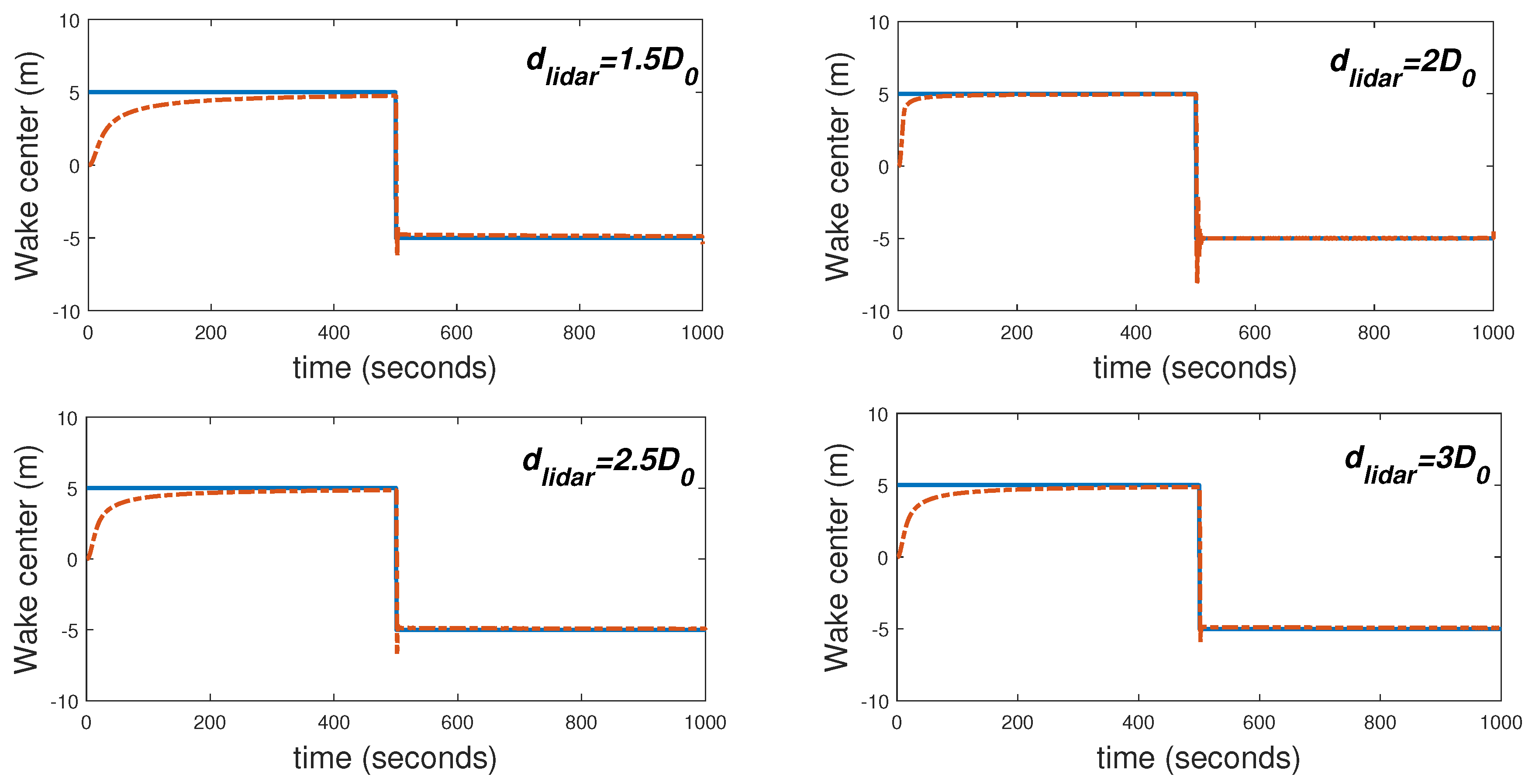
$W{T}_1$ and $W{T}_2$ are placed 400 meters apart with LiDAR at $W{T}_2$. In our simulation, the wake center trajectory at different scanning distances $d_{LiDAR}=1.5D_0,2D_0,2.5D_0$ and $3D_0$ is estimated. Based on each $d_{LiDAR}$, the wake center deflection is calculated and a transfer function is obtained for the same. The wake center calculated from different models is then allowed to track reference wake center for desired yaw angle of upwind turbine $W{T}_1$ using adaptive PI controller. Figure 12 illustrates the wake center deflection based on multi-model approach. Here the model uncertainty in form of $d_{LiDAR}$ is considered. For $d_{LiDAR}=2D_0$, the control action achieved is smooth and fast when compared to others.

Furthermore, wake center in case of multiple wake effect is estimated for wind farm layouts with 5 turbines as shown in Figure 13. The wake center is estimated for wind turbines $W{T}_4$ and $W{T}_5$ based on effective velocity deficit caused by the respective upwind turbines. Wind turbine $W{T}_4$ sees wake effect from $W{T}_1$ and $W{T}_2$. Similarly, wind turbine $W{T}_5$ experiences wake effect from $W{T}_1$, $W{T}_3$ and $W{T}_4$. The downstream distances for the upwind turbines are illustrated in terms of rotor diameter ($D_0$). The velocity deficit due to individual upwind turbine is calculated using (15) based on Gaussian deficit proposed by Bastankhah and Porté-Agel [33]. Furthermore, the deficit is determined for $W{T}_4$ and $W{T}_5$ considering upwind turbines in yawed condition, so as to deflect wake stream behind rotor.

Table 2. Wind turbine Parameters for $W{T}_4$ and $W{T}_5$.

Parameter	Value
Rotor diameter ($D_0$)	80 m
Wake growth factor (k)	0.0075
Model parameter ($k_d$)	0.15
Thrust coefficient ($C_T$)	0.888
${\gamma }_1$	[$-5^{\circ }$, $5^{\circ }$]
${\gamma }_2$	[$-{10}^{\circ }$, ${10}^{\circ }$]
${\gamma }_3$	[$-{25}^{\circ }$, ${25}^{\circ }$]
${\gamma }_4$	[$-{15}^{\circ }$, ${15}^{\circ }$]

highlights various parameters and their values used to compute effective velocity deficit with yaw angle ${\gamma }_j$ for $j\in [1,2,3,4]$.

The effective velocity deficit in yawed condition for $W{T}_4$ and $W{T}_5$ is calculated using (14) based on quadratic superposition principle. The transfer function model is built to estimate wake center deflection as shown in Figure 3. The system identification toolbox is used to estimate the overall transfer function with yaw angle being input and effective wake center calculated using (19) as the output. In Figure 3, N represents the total number of upwind turbines.

Figure 14 represents the wake center estimation for $W{T}_1$ and $W{T}_2$ which are upwind turbines for $W{T}_4$. The wake center for $W{T}_1$ and $W{T}_2$ is estimated and then controlled using adaptive PI-controller for desired yaw angle as listed in Table 2. In Figure 14, $y_{c1}^{ref},y_{c2}^{ref}$ refer to the reference wake centers for turbines $W{T}_1$ and $W{T}_2$ respectively. Similarly for $W{T}_5$, the wake center for upwind turbines $W{T}_1$, $W{T}_3$ and $W{T}_4$ is estimated and controlled using am adaptive PI-controller.

Figure 15 illustrates the reference and estimated wake centers for $W{T}_1$ and $W{T}_4$ based on transfer function model.

7. Conclusions

The LiDAR based closed-loop adaptive control for desired yaw angle is studied for a two turbine wind farm layout. Closed-loop adaptive control technique is based on identifying the transfer function for wind turbine model which gives an actual yaw angle as the output and wake center estimation model which determines the nominal wake center position. The transfer functions are obtained using system identification toolbox available in MATLAB/Simulink. The estimated wake center is computed at a distance of $1D_0$ and an Adaptive PI controller is applied in order to track a desired reference wake center. The yaw angle correction thus applied is then reflected on the wind farm power improvement by an increase of 7.552%. Furthermore, the effective air turbulence due to wake effect is studied and its was found that yaw angle adjustment reduces the turbulence on downwind turbine $W{T}_2$, with maximum turbulence occurring at $\gamma =0^{\circ }$. The study is further extended for multi-model approach where the different models pertaining to different LiDAR scanning distances are used and wake center is controlled using adaptive-PI controllers. Wake center is estimated and controlled further for a wind farm layout with 5 turbines based on transfer function model for effective velocity deficit to effective wake center. In future, the study can be extended for a wind farm operating in Ekman layer where the Coriolis force is dominant in turbulent wakes.

References

- Beyer, F.; Luhmann, B.; Raach, S.; Stuttgarter, P.W.C. Shadow Effects in an Offshore Wind Farm—Potential of Vortex Methods for Wake Modelling. In Proceedings of the Twelfth German Wind Energy Conference DEWEK, Bremen, Germany, 19–20 May 2015. [Google Scholar]
- Raach, S.; Schlipf, D.; Borisade, F.; Cheng, P.W. Wake redirecting using feedback control to improve the power output of wind farms. In Proceedings of the 2016 American Control Conference (ACC), Boston, MA, USA, 6–8 July 2016. [Google Scholar]
- Campagnolo, F.; Petrović, V.; Schreiber, J.; Nanos, E.M.; Croce, A.; Bottasso, C.L. Wind tunnel testing of a closed-loop wake deflection controller for wind farm power maximization. J. Phys. Conf. Ser. 2016, 753, 032006. [Google Scholar] [CrossRef] [Green Version]
- Howland, M.F.; Bossuyt, J.; Martínez-Tossas, L.A.; Meyers, J.; Meneveau, C. Wake structure in actuator disk models of wind turbines in yaw under uniform inflow conditions. J. Renew. Sustain. Energy 2016, 8, 043301. [Google Scholar] [CrossRef] [Green Version]
- Gebraad, P.M.O.; Teeuwisse, F.; van Wingerden, J.; Fleming, P.A.; Ruben, S.D.; Marden, J.R.; Pao, L.Y. A data-driven model for wind plant power optimization by yaw control. In Proceedings of the 2014 American Control Conference, Portland, OR, USA, 4–6 June 2014. [Google Scholar]
- Fleming, P.A.; Gebraad, P.M.; Lee, S.; van Wingerden, J.W.; Johnson, K.; Churchfield, M.; Michalakes, J.; Spalart, P.; Moriarty, P. Evaluating techniques for redirecting turbine wakes using SOWFA. Renew. Energy 2014, 70, 211–218. [Google Scholar] [CrossRef]
- Adaramola, M.; Krogstad, P.Å. Experimental investigation of wake effects on wind turbine performance. Renew. Energy 2011, 36, 2078–2086. [Google Scholar] [CrossRef]
- Maeda, T.; Yokota, T.; Shimizu, Y.; Adachi, K. Wind Tunnel Study of the Interaction between Two Horizontal Axis Wind Turbines. Wind Eng. 2004, 28, 197–212. [Google Scholar] [CrossRef]
- Dar, Z.; Kar, K.; Sahni, O.; Chow, J.H. Windfarm Power Optimization Using Yaw Angle Control. IEEE Trans. Sustain. Energy 2017, 8, 104–116. [Google Scholar] [CrossRef]
- Raach, S.; Schlipf, D.; Cheng, P.W. Lidar-based wake tracking for closed-loop wind farm control. J. Phys. Conf. Ser. 2016, 753, 052009. [Google Scholar] [CrossRef] [Green Version]
- Doubrawa, P.; Barthelmie, R.; Wang, H.; Pryor, S.; Churchfield, M. Wind Turbine Wake Characterization from Temporally Disjunct 3-D Measurements. Remote Sens. 2016, 8, 939. [Google Scholar] [CrossRef]
- Doubrawa, P.; Barthelmie, R.J.; Wang, H.; Churchfield, M.J. A stochastic wind turbine wake model based on new metrics for wake characterization. Wind Energy 2016, 20, 449–463. [Google Scholar] [CrossRef]
- Wang, H.; Barthelmie, R.J.; Doubrawa, P.; Pryor, S.C. Errors in radial velocity variance from Doppler wind LiDAR. Atmos. Meas. Tech. 2016, 9, 4123–4139. [Google Scholar] [CrossRef]
- Ioannou, P.A.; Sun, J. Robust Adaptive Control; Prentice-Hall, Inc.: Upper Saddle River, NJ, USA, 1995. [Google Scholar]
- Landau, I.D.; Lozano, R.; M’Saad, M.; Karimi, A. Adaptive Control; Springer: London, UK, 2011. [Google Scholar] [CrossRef]
- Nguyen, N.T. Model-Reference Adaptive Control; Springer International Publishing: Basel, Switzerland, 2018. [Google Scholar] [CrossRef]
- Chen, C.T. Direct Adaptive Control of Chemical Process Systems. Ind. Eng. Chem. Res. 2001, 40, 4121–4140. [Google Scholar] [CrossRef]
- Deb, D.; Tao, G.; Burkholder, J.; Smith, D. Adaptive Synthetic Jet Actuator Compensation for A Nonlinear Aircraft Model at Low Angles of Attack. IEEE Trans. Control Syst. Technol. 2008, 16, 983–995. [Google Scholar] [CrossRef]
- Deb, D.; Tao, G.; Burkholder, J.; Smith, D. An adaptive inverse control scheme for a synthetic jet actuator model. In Proceedings of the 2005 American Control Conference, Portland, Oregon, 8–10 June 2005. [Google Scholar]
- Nath, A.; Deb, D.; Dey, R.; Das, S. Blood glucose regulation in type 1 diabetic patients: An adaptive parametric compensation control-based approach. IET Syst. Biol. 2018, 12, 219–225. [Google Scholar] [CrossRef]
- Patel, R.; Deb, D. Parametrized control-oriented mathematical model and adaptive backstepping control of a single chamber single population microbial fuel cell. J. Power Sources 2018, 396, 599–605. [Google Scholar] [CrossRef]
- Vollmer, L.; Steinfeld, G.; Heinemann, D.; Kühn, M. Estimating the wake deflection downstream of a wind turbine in different atmospheric stabilities: An LES study. Wind Energy Sci. 2016, 1, 129–141. [Google Scholar] [CrossRef]
- Simley, E.; Pao, L.; Frehlich, R.; Jonkman, B.; Kelley, N. Analysis of Wind Speed Measurements using Continuous Wave LiDAR for Wind Turbine Control. In Proceedings of the 49th AIAA Aerospace Sciences Meeting including the New Horizons Forum and Aerospace Exposition. American Institute of Aeronautics and Astronautics, Orlando, FL, USA, 4–7 January 2011. [Google Scholar]
- Schlipf, D.; Schlipf, D.J.; Kühn, M. Nonlinear model predictive control of wind turbines using LiDAR. Wind Energy 2012, 16, 1107–1129. [Google Scholar] [CrossRef]
- Bianchi, F.D.; Mantz, R.J.; Battista, H.D. Wind Turbine Control Systems; Springer: London, UK, 2007. [Google Scholar]
- Fleming, P.; Annoni, J.; Shah, J.J.; Wang, L.; Ananthan, S.; Zhang, Z.; Hutchings, K.; Wang, P.; Chen, W.; Chen, L. Field test of wake steering at an offshore wind farm. Wind Energy Sci. 2017, 2, 229–239. [Google Scholar] [CrossRef] [Green Version]
- Jonkman, J.; Butterfield, S.; Musial, W.; Scott, G. Definition of a 5-MW Reference Wind Turbine for Offshore System Development; Technical report; National Renewable Energy Lab. (NREL): Golden, CO, USA, 2009. [Google Scholar]
- Qian, G.W.; Ishihara, T. A New Analytical Wake Model for Yawed Wind Turbines. Energies 2018, 11, 665. [Google Scholar] [CrossRef]
- Jiménez, Á.; Crespo, A.; Migoya, E. Application of a LES technique to characterize the wake deflection of a wind turbine in yaw. Wind Energy 2009, 13, 559–572. [Google Scholar] [CrossRef]
- Manwell, J.F.; McGowan, J.G.; Rogers, A.L. Wind Energy Explained; John Wiley & Sons, Ltd.: Hoboken, NJ, USA, 2009. [Google Scholar]
- Machefaux, E.; Larsen, G.C.; Troldborg, N.; Gaunaa, M.; Rettenmeier, A. Empirical modeling of single-wake advection and expansion using full-scale pulsed LiDAR-based measurements. Wind Energy 2014, 18, 2085–2103. [Google Scholar] [CrossRef]
- Larsen, G.; Larsen, T.; Chougule, A. Medium fidelity modelling of loads in wind farms under non-neutral ABL stability conditions—A full-scale validation study. J. Phys. Conf. Ser. 2017, 854, 012026. [Google Scholar] [CrossRef]
- Bastankhah, M.; Porté-Agel, F. A new analytical model for wind-turbine wakes. Renew. Energy 2014, 70, 116–123. [Google Scholar] [CrossRef]
- Katic, I.; Højstrup, J.; Jensen, N. A Simple Model for Cluster Efficiency. In Proceedings of the European Wind Energy Association Conference and Exhibition, Rome, Italy, 7–9 October 1986; Palz, W., Sesto, E., Eds.; A. Raguzzi: Rome, Italy, 1987; pp. 407–410. [Google Scholar]
- Chowdhury, S.; Zhang, J.; Messac, A.; Castillo, L. Unrestricted wind farm layout optimization (UWFLO): Investigating key factors influencing the maximum power generation. Renew. Energy 2012, 38, 16–30. [Google Scholar] [CrossRef]
- Thomsen, K.; Sørensen, P. Fatigue loads for wind turbines operating in wakes. J. Wind Eng. Ind. Aerodyn. 1999, 80, 121–136. [Google Scholar] [CrossRef]
- Scientific, C. Finance Grade Performance, ZephIR 300; Technical Report; Campbell Scientific, Inc.: Edmonton, AB, Canada, 2016. [Google Scholar]
Figure 1.
Wake center estimation for a single set of upwind and downwind turbines.
Figure 2.
Block diagram representation for wake center estimation.
Figure 3.
Wake center estimation based on transfer function in case of multiple wake scenario.
Figure 4.
Wake stream deflection caused by yaw angle misalignment.
Figure 5.
Closed loop transfer function.
Figure 6.
Modified block diagram of closed loop system.
Figure 7.
Estimated wake center and yaw angle alignment for model parameter .
Figure 8.
Wake center deflection and Wind farm power output.
Figure 9.
Yaw bearing moment and its power spectral density.
Figure 10.
Controller sensitivity for for single wake scenario.
Figure 11.
Variation of effective turbulence with yaw angle misalignment.
Figure 12.
Wake center deflection based on multi-model approach. Blue (solid) line represents reference wake center and orange (dotted) represents estimated wake center deflection.
Figure 13.
Schematic for 5 turbine wind farm layout in non-yawed and yawed condition.
Figure 14.
Wake center estimation for upwind turbines and .
Figure 15.