Performance and Design Optimization of a One-Axis Multiple Positions Sun-Tracked V-trough for Photovoltaic Applications

Abstract

In this article, the performance of an inclined north-south axis (INSA) multiple positions sun-tracked V-trough with restricted reflections for photovoltaic applications (MP-VPVs) is investigated theoretically based on the imaging principle of mirrors, solar geometry, vector algebra and three-dimensional radiation transfer. For such a V-trough photovoltaic module, all incident radiation within the angle ${\theta }_a$ arrives on solar cells after less than k reflections, and the azimuth angle of V-trough is daily adjusted M times about INSA to ensure incident solar rays always within ${\theta }_a$ in a day. Calculations and analysis show that two-dimensional sky diffuse radiation can’t reasonably estimate sky diffuse radiation collected by fixed inclined north-south V-trough, but can for MP-VPVs. Results indicate that, the annual power output (P_a) of MP-VPVs in a site is sensitive to the geometry of V-trough and wall reflectivity (ρ), hence given M, k and ρ, a set of optimal ${\theta }_a$ and $\phi$, the opening angle of V-trough, for maximizing P_a can be found. Calculation results show that the optimal ${\theta }_a$ is about 21°, 13.5° and 10° for 3P-, 5P- and 7P-VPV-k/${\theta }_a$ (k = 1 and 2), respectively, and the optimal $\phi$ for maximizing P_a is about 30° for k = 1 and 21° for k = 2when ρ > 0.8. As compared to similar fixed south-facing PV panels, the increase of annual electricity from MP-VPVs is even larger than the geometric concentration of V-trough for ρ > 0.8 in sites with abundant solar resources, thus attractive for water pumping due to stable power output in a day.

1. Introduction

Energy is essential for the daily life of human beings, but extensive use and exploitation has resulted in severe environmental and ecological consequences, hence direct use of solar energy for electricity and heat generation is becoming more attractive. In recent years, low temperature solar thermal techniques have been widely used for water and building heating, but applications of photovoltaic technology are limited due to the high cost of electricity from PV systems although the cost of solar cells has decreased dramatically in recent years [1,2,3]. Potential ways to reduce the cost of electricity from a PV system include the use of sun-tracking techniques and cheap optical concentrators. Continuous sun-tracking can increase the power output from PV systems, but sophisticated sun-tracking and control devices are required [4]. In recent years, low concentrators such as compound parabolic concentrators (CPCs) and V-trough concentrators have been widely tested for concentrating radiation on solar cells. Compared with similar PV panels, a low concentrated PV system could reduce cost of electricity by up to 40% [5]. Mallick et al. tested an asymmetric CPC ($\times$2.01)-based photovoltaic module for building integration, and an increase of 62% in maximum power point was observed as compared to similar non-concentrating solar panels [6,7]. A comparative study by Yousef et al. under hot and arid climatic conditions showed that, in comparison with similar solar panels, the electricity generated by a CPC (2.4$\times$)-based CPV system with and without cooling of solar cells was 52% and 33% higher, respectively [8]. To increase the geometric concentration and reduce the optical losses of reflective CPCs due to imperfect reflections, dielectric totally internally reflecting CPCs were tested and studied in recent years [9,10,11,12]. An experiment by Muhammad-Sukki et al. showed that the use of a mirror symmetrical dielectric CPC (4.9$\times$) increased the power output of solar cells by a factor of 4.2 [3]. Studies by Yu et al. [13] and Baig et al. [14] showed that, for low concentrating PV systems, uneven irradiation on solar cells did not have significant effects on the CPV power output, but the incidence angle (IA) on solar cells had an significant effect when the IA is larger than 45°.

Compared to CPCs, V-trough concentrators are extremely easy to fabricate, the solar irradiation on the base of V-trough is more uniform and the unused heat is more easily dissipated through the side walls, thus making them more suitable for concentrating radiation on commercially available solar cells. Experimental studies by Sangani and Solanki showed that a V-trough concentrator ($\times$2) increased power output by 44%, and the cost of electricity was reduced by 24% as compared to similar PV panels [15]. Solanki et al. tested a V-trough-based PV system (VPV) where the V-trough was fabricated from a single aluminum sheet, and found that the cell temperature was almost identical to that of a non-concentrated PV module [16].

Theoretical and experimental studies showed that an appropriately designed VPV was particularly adequate for water pumping due to the uniform irradiation on the solar cells [17]. A study by Bione et al. showed that the one-axis sun-tracked VPV ($\times$2.2) increased the annual volume of pumped water by a factor of 2.49 as compared to similar fixed solar panels [18], larger than the geometric concentration of the V-trough. With an array of 1.3 kWp, Bione et al. found that the VPV water pumping system was able to irrigate 2.11 ha of grapes, but a similar fixed photovoltaic array only irrigated 1.2 ha under the climatic conditions of Petrolina, Brazil [19].

A pump directly driven by the electricity from PV modules works only when the incident radiation is above the level required to start the pump, thus to make radiation on PV panels higher than the critical level, one of best solutions is to track the Sun [20]. However, continuous sun-tracking PV systems often suffer from mechanical failures. Huang and Sun first proposed the design of a one-axis three-position sun-tracking PV system [21], and their calculations showed that the annual power output increased about 37.5% as compared to fixed PV panels in an area with abundant solar resources [22,23]. A study by Zhong et al. indicated that the annual solar gain on 3-position sun-tracked solar panels was above 96% of that collected by 2-axis tracked PV panels [24]. These studies show that one-axis 3-position sun-tracking techniques can greatly increase the power output of PV systems.

The V-trough is not an ideal solar concentrator, thus the increase of power output from VPVs is limited because, with the increase of geometric concentration (C_g) of a V-trough, more radiation is lost due to imperfect multiple reflections of solar rays on their way to the absorber [25]. To improve the optical performance of V-troughs, the reflections of solar rays on way to solar cells should be restricted, and for such VPV module (VPV-k/θ_a), all radiation within the angle θ_a is required to arrive on solar cells after less than k reflections. Similar to trough-like CPCs, the optical performance of V-troughs is uniquely determined by the projected incidence angle (θ_p) of solar rays on the cross-section of the V-trough [26,27,28], thus two-dimensional radiation transfer, where radiation transfer on the cross-section is considered, can reasonably predict the optical performance [28]. However, the 2-D model can’t reasonably predict photovoltaic performance as the photovoltaic efficiency of solar cells is sensitive to the IA instead of θ_p [13].

In this work, a new design concept, the INSA multiple-position sun-tracked V-trough with restricted reflections (MP-VPV-k/θ_a), is proposed for potential photovoltaic water pumping applications. The design of MP-VPV-k/θ_a is that the V-trough is oriented in the north-south direction and inclined from the horizon. To ensure θ_p is always within θ_a in a day, the azimuth angle of the aperture is daily adjusted several times (M) from eastward in the morning to westward in the afternoon by rotating V-trough 2θ_a about INSA once when θ_p = θ_a. To theoretically investigate the performance of MP-VPV-k/θ_a, a mathematical procedure is suggested based on the imaging principles of mirrors, solar geometry, vector algebra and three-dimensional radiation transfer with the aim to find the optimal design of such VPV for maximizing its annual electricity generation.

2. Design of MP-VPV-k/θ_a

2.1. Geometry of VPV-k/θ_a

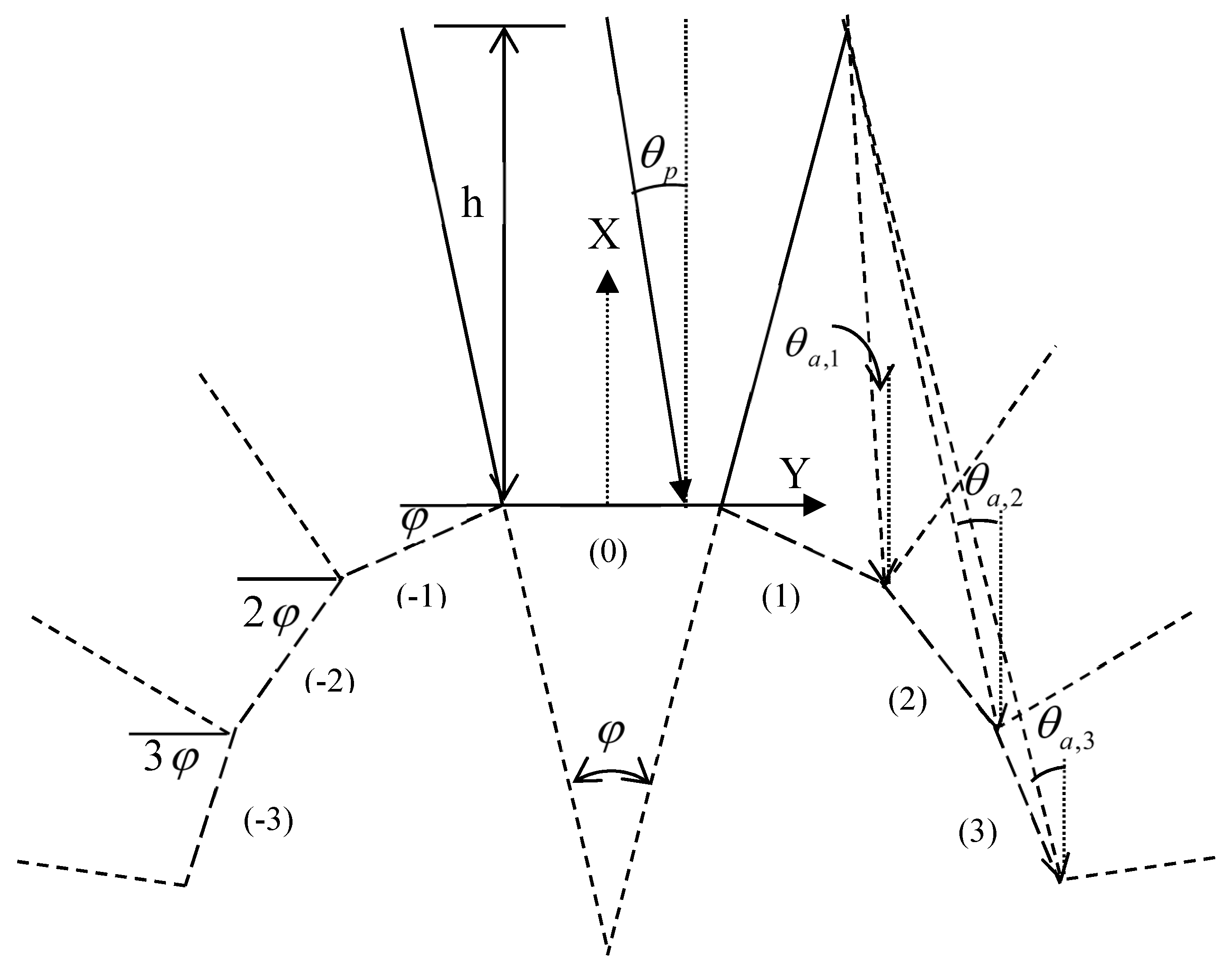
As shown in Figure 1, according to the imaging principle of mirrors, solar rays “irradiating“ on the ith left/right image of the base will arrive on the base after i reflections [25]. Therefore, when a beam of radiation is incident on the aperture of V-trough at θ_p ≤ θ_a,1, all radiation irradiating on right reflector arrives on the base after one reflection. Similarly, all radiation irradiating on the right reflector at θ_p ≤ θ_a,k (k = 1, 2, 3…) arrives on the base after less than k reflections. The geometry of VPV-k/${\theta }_a$ is subject to:

C_g = sin[(k + 0.5)φ + θ_a]/sin(0.5φ + θ_a)

(1)

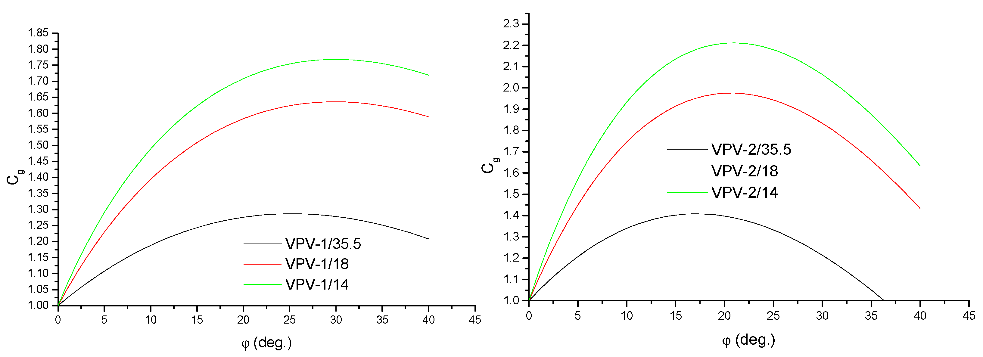
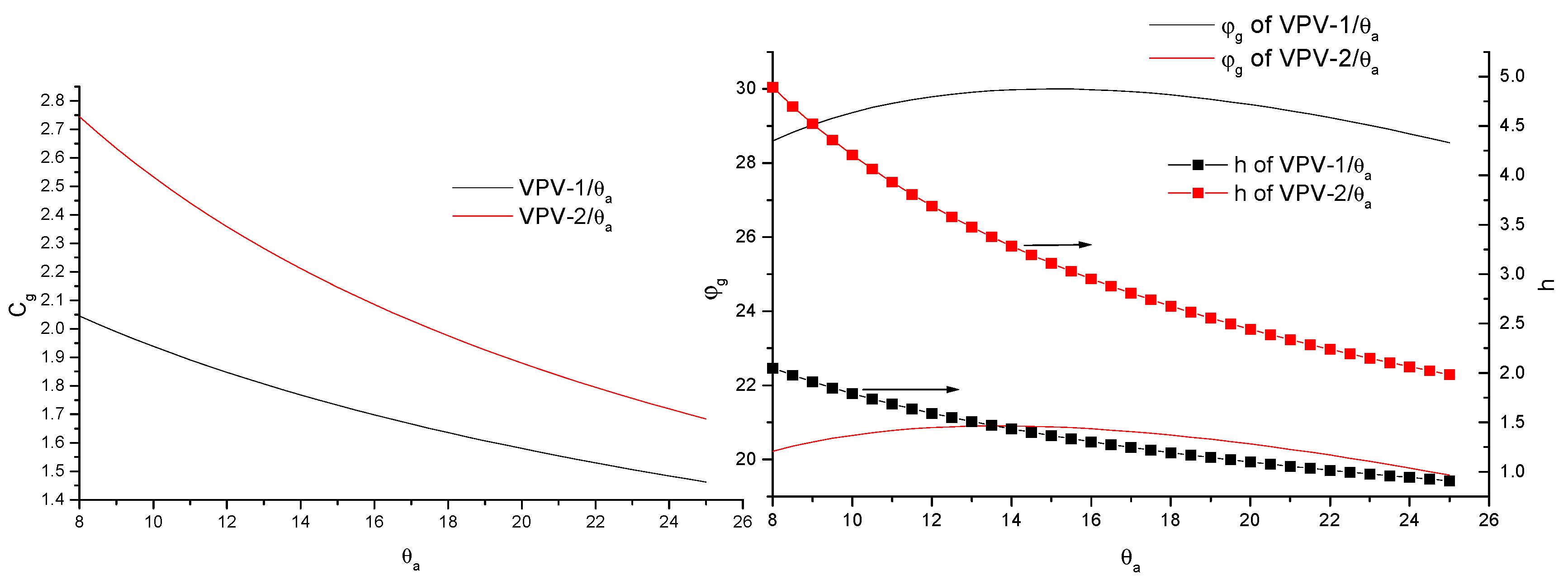
where $\phi$ is the opening angle of V-trough, and the height of V-trough is h = 0.5(C_g − 1)/tan(0.5$\phi$). It is known from Equation (1) that the geometric concentration C_g of VPV-k/${\theta }_a$ depends on k, ${\theta }_a$ and $\phi$, hence given k and ${\theta }_a$, ${\phi }_g$, the optimal $\phi$ for maximizing $C_g$, can be found. It is seen from Figure 2 that, given k, a different ${\theta }_a$ yields a different ${\phi }_g$ thus different optimal geometry of VPV-k/${\theta }_a$ for maximizing C_g. As shown in Figure 3, with the increase of ${\theta }_a$, C_g and h of VPV-k/${\theta }_a$ optimized for maximizing C_g decrease, and ${\phi }_g$ increases first then decreases. It is known from Figure 3 that the ${\phi }_g$ varies around 30° for k = 1 and 21° for k = 2 as 8° < ${\theta }_a$ < 25°.

2.2. Description of MP-VPV-k/θ_a

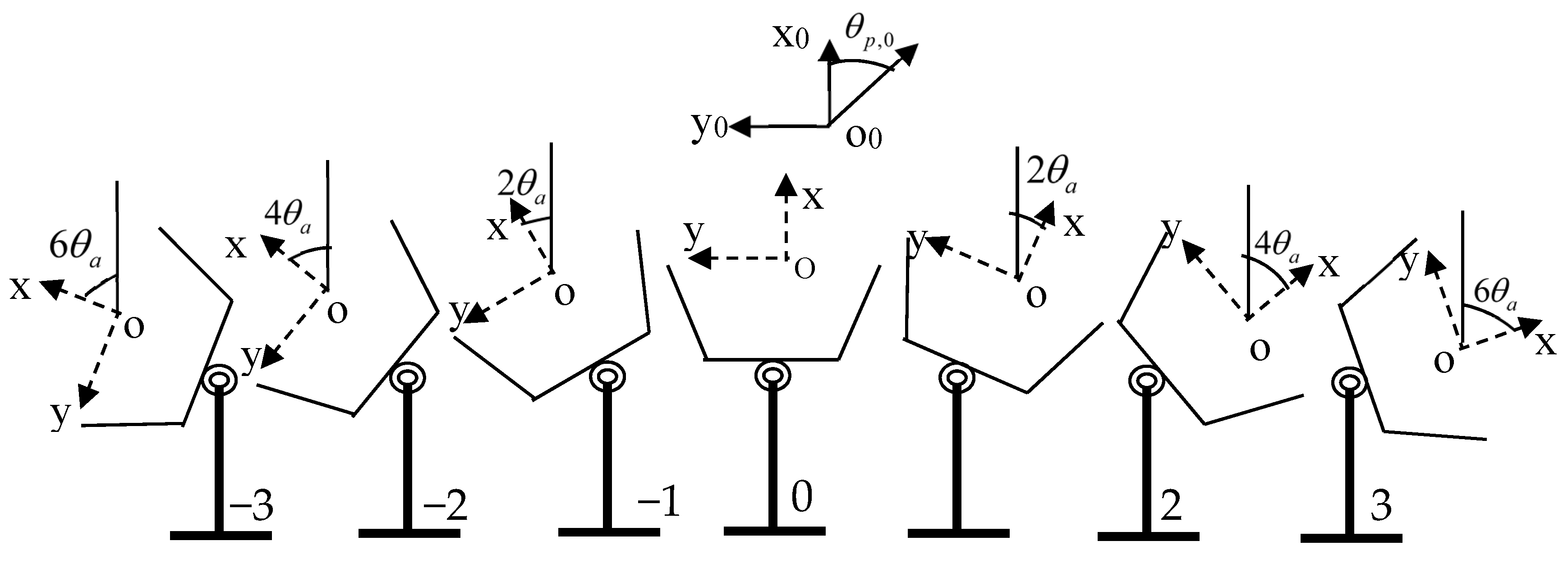
As shown in Figure 4, the VPV-k/θ_a is oriented in the north-south direction and inclined at β from the horizon. To make θ_p always be with θ_a in a day, a multiple-position Sun-tracking strategy is required. In the early morning, the aperture is adjusted eastward, $\gamma$ = (M − 1)${\theta }_a$ from due south, then the azimuth angle is successively adjusted once when θ_p = θ_a by rotating the V-trough 2${\theta }_a$ about INSA from east to west. The azimuth angle adjustment can be automatically conducted by a computerized mechanical device controlled by solar time or a photosensor.

3. Optical and Photovoltaic Efficiency of MP-VPV-k/θ_a

3.1. Coordinate Systems Used in This Work

To be convenient for the analysis, two coordinate systems, (x₀,y₀, z₀) and (x,y,z), are employed in this work. As shown in Figure 4, both coordinate systems are fixed on the aperture of the V-trough with the x₀/x-axis normal to the aperture, and the z₀/z-axis parallel to INSA and pointing to the northern sky dome. The (x₀,y₀,z₀) system is fixed on the aperture of the V-trough at the solar-noon Sun-tracking position, thus the y₀-axis always points due east; whereas the (x,y,z) system is fixed on the aperture of the sun-tracked V-trough, thus the direction of y-axis varies during a day. In the (x₀,y₀,z₀) coordinate system, the incident solar rays at any time of a day can be expressed by a unit vector from Earth to the Sun as follows [28,29]:

$$n_{s,0}=(n_{x0},n_{y0},n_{z0})$$

(2)

where:

$$\{\begin{array}{l}{n}_{x0}=\cos \delta \cos \omega \cos (\lambda -\beta )+\sin \delta \sin (\lambda -\beta )\hfill \\ n_{y0}=-\cos \delta \sin \omega \hfill \\ n_{z0}=-\cos \delta \cos \omega \sin (\lambda -\beta )+\sin \delta \cos (\lambda -\beta )\hfill \end{array}$$

(3)

where $\lambda$ is the site latitude, $\omega$ the solar hour angle, and $\delta$ the declination of the Sun and varies with the day number counting from first day of a year [29]. The projected angle of solar rays on the cross-section of V-trough relative to x₀-axis is given by:

$${\theta }_{p,0}=\{\begin{array}{ll}Atn\left|n_{y0}/n_{x0}\right|\hfill & (n_{x0}>0)\hfill \\ 0.5\pi \hfill & (n_{x0}=0)\hfill \\ 0.5\pi +Atn\left|n_{x0}/n_{y0}\right|\hfill & (n_{x0}<0)\hfill \end{array}$$

(4)

In the coordinate system (x, y, z), the unit vector from Earth to the Sun, $n_s$ = ($n_x$, $n_y$, $n_z$), is expressed by:

$$\{\begin{array}{l}{n}_x=n_{x0}\cos {\gamma }_i-n_{y0}\sin {\gamma }_i\hfill \\ n_y=n_{x0}\sin {\gamma }_i+n_{y0}\cos {\gamma }_i\hfill \\ n_z=n_{z0}\hfill \end{array}$$

(5)

as the coordinate system (x, y, z) is obtained by rotating the coordinate system (x₀,y₀,z₀)${\gamma }_i$ about z₀-axis. The ${\gamma }_i$ in Equation (5), the azimuth angle of V-trough at the i-th Sun-tracking position relative to x₀-axis, positive in the afternoon, is determined by M, ${\theta }_{p,0}$ and ${\theta }_a$. As an example, for 7P-VPV-k/${\theta }_a$, it is given by:

$${\gamma }_i=\{\begin{array}{cc}0& ({\theta }_{p,0}\le {\theta }_a)\\ 2{\theta }_a& ({\theta }_a<{\theta }_{p,0}\le 3{\theta }_a)\\ 4{\theta }_a& (3{\theta }_a<{\theta }_{p,0}\le 5{\theta }_a)\\ 6{\theta }_a& ({\theta }_{p,0}>5{\theta }_a)\end{array}$$

(6)

The optical and photovoltaic performance of VPVs for solar rays $n_s$ = ($n_x$, $\pm$$n_y$, $n_z$) are identical due to the symmetric geometry, hence $n_s$ = ($n_x$, −$\left|n_y\right|$, $n_z$) is used in this exercise for simplifying analysis, namely solar rays are always assumed to be incident onto the right reflector. The projected incident angle of solar rays on the aperture of V-trough is given by:

$$\tan {\theta }_p=\left|n_y/n_x\right|\mathrm{or}{\theta }_p=\left|{\theta }_{p,0}-{\gamma }_i\right|$$

(7)

The unit vector of normal to the horizon in the (x₀,y₀,z₀) system is expressed by:

$$n_{h,0}=(\cos \beta ,0,\sin \beta )$$

(8)

Also, in the (x, y, z) system, it is given based on Equation (5) as:

$$n_h=(\cos \beta \cos {\gamma }_i,\cos \beta \sin {\gamma }_i,\sin \beta )$$

(9)

3.2. Optical and Photovoltaic Efficiency of MP-VPV-k/θ_a

To simplify the analysis, it is assumed that the length of the V-trough is infinite as compared to the width (it is set to be 1), and side-walls are perfect specular and gray surfaces. When a beam of radiation is incident on the aperture at θ_p, a fraction of the radiation directly irradiates on the solar cells, and the remainder arrives on the solar cells after reflections from both walls. Therefore, the collectible radiation on solar cells at any time in a day includes three parts: radiation directly irradiating on the solar cells (I₁), and radiation incident on the right/left wall and arriving on solar cells after multiple reflections (I₂/I₃). Thus, the optical efficiency of the V-trough is expressed by:

$$f=(I_1+I_2+I_3)/I_{ap}=f_1+f_2+f_3$$

(10)

where I_ap is the radiation incident on the aperture, $f_1$, $f_2$ and $f_3$ are the energy fractions of radiation on the solar cells contributed by I₁, I₂ and I₃, respectively. Similarly, the photovoltaic efficiency of VPVs is given by:

$$\eta =(P_1+P_2+P_3)/I_{ap}={\eta }_1+{\eta }_2+{\eta }_3$$

(11)

where P_i (i = 1,2,3) is the electricity generated by I_i (i = 1,2,3), and ${\eta }_i$ is the photovoltaic efficiency contributed by P_i.

3.2.1. Calculation of f₁ and η₁

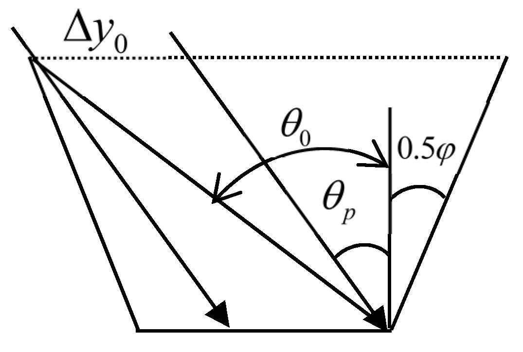
As shown in Figure 5, the base of the V-trough is fully irradiated as ${\theta }_p$ $\le$ 0.5$\phi$, partially irradiated as 0.5$\phi$ < ${\theta }_p$ < ${\theta }_0$, and fully shaded by the left wall as ${\theta }_p$ $\ge$ ${\theta }_0$. Hence, the energy fraction of radiation directly incident on the base is given by:

$$f_1=\frac{\Delta y_0}{A_{ap}}=\frac{\Delta y_0}{C_g}\{\begin{array}{ll}1/C_g\hfill & ({\theta }_p\le 0.5\phi )\hfill \\ h(\tan {\theta }_0-\tan {\theta }_p)\hfill & (0.5\phi <{\theta }_p\le {\theta }_0)\hfill \\ 0\hfill & ({\theta }_p>{\theta }_0)\hfill \end{array}$$

(12)

where A_ap = C_g is the width of the aperture, and ${\theta }_0$ (shown in Figure 5) is given by:

$$\tan {\theta }_0=0.5(1+C_g)/h$$

(13)

The IA of solar rays directly irradiating on solar cells, ${\theta }_{in,0}$, is given by:

$$\cos {\theta }_{in,0}=n_s·n_{base}=n_s·(1,0,0)=n_x$$

(14)

as the vector of normal to the base is $n_{base}$ = (1,0,0) in the system (x,y,z). Therefore, η₁ is given by:

$${\eta }_1=\Delta y_0{\eta }_{pv}({\theta }_{in,0})/C_g=f_1{\eta }_{pv}({\theta }_{in,0})$$

(15)

where ${\eta }_{pv}({\theta }_{in,0})$ is the photovoltaic efficiency of the solar cells as a function of ${\theta }_{in,0}$. The electricity from VPVs is commonly affected by many factors such as cell temperature, IA and solar flux distribution [14,30]. To investigate the effects of the geometry of the V-trough on power generation from VPVs, it is assumed that, except for IA, the effects of all other factors on the photovoltaic efficiency of VPVs with different geometry are identical, and the photovoltaic efficiency of solar cells is subjected to the correlation suggested by Yu et al., expressed as [13]:

$${\eta }_{pv}=\{\begin{array}{ll}15.5494+0.02325{\theta }_{in}-0.00301{\theta }_{in}^2+9.4685\times {10}^{-5}{\theta }_{in}^3-1.134\times {10}^{-6}{\theta }_{in}^4\hfill & (0<{\theta }_{in}<65°)\hfill \\ 41.52-0.4784{\theta }_{in}\hfill & (65°\le {\theta }_{in}<90°)\hfill \end{array}$$

(16)

3.2.2. Calculation of f₂ and η₂

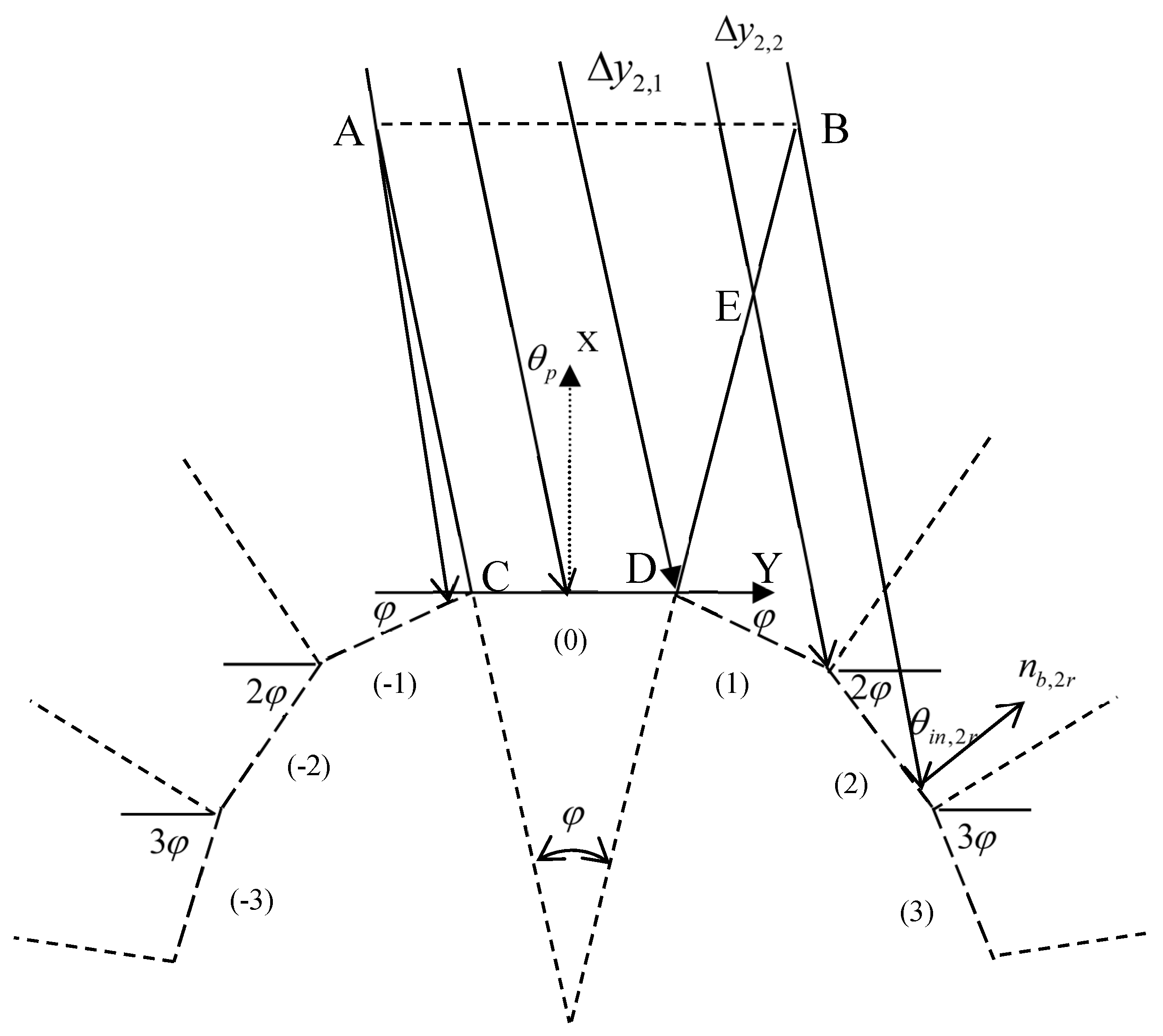
As shown in Figure 6, when solar rays are incident on the right wall of V-trough, the radiation incident on the lower part of reflector (DE) “irradiates” on the first image of base thus arrives on solar cells after one reflection, and radiation incident on the upper part of reflector (BE) “irradiates” on 2nd image hence arrives on solar cells after two reflections. Therefore, the energy fraction of radiation incident on right reflector and arriving on solar cells is given by:

$$f_2={\displaystyle \sum _{k=1}^n\Delta y_{2,k}}{\rho }^k/C_g$$

(17)

where n is the maximum reflection number of solar rays on way to solar cells, and is the integer of 90/$\phi$ or 90/$\phi$ − 1 when 90/$\phi$ is an integer [25], $\rho$ is the reflectivity of the side walls of the V-trough, and $\Delta y_{2,k}$ is the radiation “irradiating” on the kth right image and calculated based on the method given in Appendix A. The photovoltaic efficiency of VPVs due to the contribution of I₂ is calculated by:

$${\eta }_2={\displaystyle \sum _{k=1}^n\Delta y_{2,k}\eta ({\theta }_{in,kr})}{\rho }^k/C_g$$

(18)

where ${\theta }_{in,kr}$ is the IA of solar ray on the kth right image, and can be calculated by:

$$\cos {\theta }_{in,kr}=n_s·n_{b,kr}=n_x\cos k\phi +n_y\sin k\phi$$

(19)

as the vector of normal to kth right image is $n_{b,kr}$ = (cos$k\phi$, sin$k\phi$, 0) in the (x,y,z) system.

3.2.3. Calculation of f₃ and η₃

Similarly, the energy fraction of radiation incident on the left wall of the V-trough and arriving on solar cells after multiple reflections is calculated by:

$$f_3={\displaystyle \sum _{k=1}^n\Delta y_{3,k}}{\rho }^k/C_g$$

(20)

where $\Delta y_{3,k}$ is the radiation “irradiating” on the kth left image, calculated based on the method given in Appendix B. The photovoltaic efficiency of VPVs due to the contribution of I₃ is calculated by:

$${\eta }_3={\displaystyle \sum _{k=1}^n\Delta y_{3,k}\eta ({\theta }_{in,kl})}{\rho }^k/C_g$$

(21)

where ${\theta }_{in,kl}$ is the IA of solar rays on the kth left image, and calculated by:

$$\cos {\theta }_{in,kl}=n_s·n_{b,kl}=n_x\cos k\phi -n_y\sin k\phi$$

(22)

as the vector of normal to kth left image of base is $n_{b,kl}$ = (cosk$\phi$, −sink$\phi$, 0) in the (x,y,z) system.

The analysis above shows that the f of VPVs is uniquely determined by ${\theta }_p$, thus it is a function of ${\theta }_p$, but the $\eta$ is dependent on ${\theta }_p$ and the IA of solar rays on the aperture of the V-trough (${\theta }_{ap}$) since the ${\theta }_{ap}$ is given by cos${\theta }_{ap}$ = $n_s$ $·$ (1, 0, 0) = $n_x$.

3.3. Collectible Radiation and Power Generation of MP-VPV-k/θ_a

In the case radiation reflecting from the ground is neglected, the collectible radiation on a unit area of solar cells of MP-VPV-k/${\theta }_a$ at any time of a day is calculated by:

$$I_{base}=C_g{I}_{b}g({\theta }_{ap})f\cos {\theta }_{ap}+I_{base,d}=C_g{I}_{b}g({\theta }_{ap})n_{x}f+I_{base,d}$$

(23)

where I_b is the intensity of the beam radiation, and $g({\theta }_{ap})$ is a control function, being 1 for cos${\theta }_{ap}$ > 0 and otherwise zero. The electricity generated by unit area of solar cells is expressed by:

$$P=C_g{I}_{b}g({\theta }_{ap})cos{\theta }_{ap}\eta +P_d=C_g{I}_{b}g({\theta }_{ap})n_x\eta +P_d$$

(24)

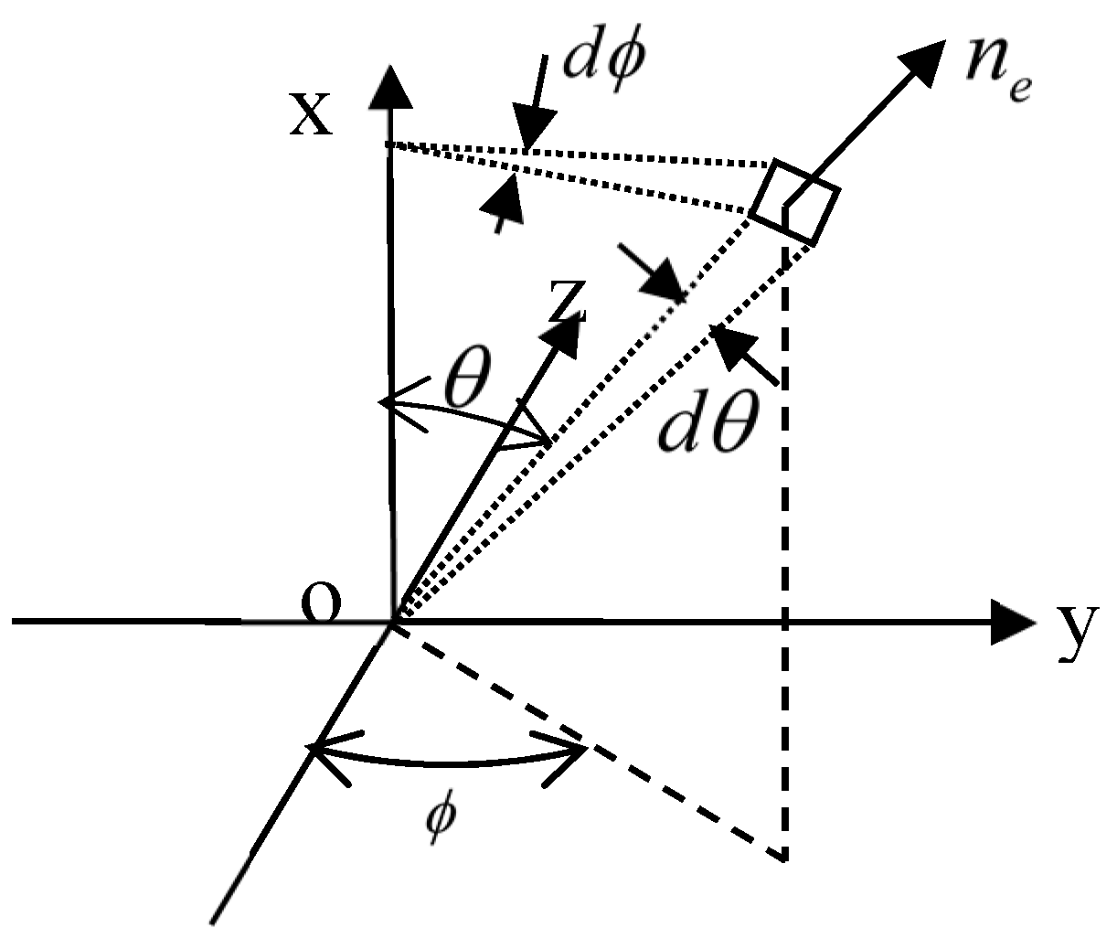
The term $I_{base,d}$ in Equation (23), the collectible sky diffuse radiation of the V-trough, is dependent on the sky dome “seen” from the aperture of MP-VPVs, and $P_d$ in Equation (24) is the electricity generated by $I_{base,d}$. To calculate $I_{base,d}$ and $P_d$, it is assumed that diffuse radiation from all directions of the sky dome is identical. In the coordinate system (x,y,z), the sky diffuse radiation on a unit area of solar cells from a finite element on the sky dome (see Figure 7) is:

$$d{I}_{base,d}=C_g{i}_d\cos \theta fg({\theta }_{e-h})d\Omega$$

(25)

and the power generated by $d{I}_{base,d}$ is expressed by:

$$d{P}_d=C_g{i}_d\cos \theta \eta g({\theta }_{e-h})d\Omega$$

(26)

where $d\Omega$ = sin$\theta$$d\theta$$d\varphi$ is the solid angle covered by the finite element; $i_d$, the directional intensity of the sky diffuse radiation, is equal to $I_d$/$\pi$ for isotopic sky diffuse radiation [28]; and $I_d$ is the sky diffuse radiation on the horizon. The ${\theta }_{e-h}$ is the IA on the horizon for sky diffuse radiation from element $d\Omega$, and $g({\theta }_{e-h})$ is a control function, being 1 for cos${\theta }_{e-h}$ > 0 and 0 for cos${\theta }_{e-h}$ < 0 because the sky element is below the ground level in this case. The vector of sky diffuse radiation from element $d\Omega$ (see Figure 7) is expressed by:

$$n_e=\left(\cos \theta , \sin \theta \sin \varphi , -\sin \theta \cos \varphi \right)$$

(27)

Thus, the ${\theta }_{e-h}$ can be calculated based on $n_e$ and $n_h$ (given by Equation (9)) as:

$$\cos {\theta }_{e-h}=n_e·n_h=\cos \theta \cos \beta \cos {\gamma }_i+\sin \theta \sin \varphi \cos \beta \sin {\gamma }_i-\sin \theta \cos \varphi \sin \beta$$

(28)

and the projected incident angle of sky diffuse radiation from $d\Omega$ is given by:

$$\tan {\theta }_p=\left|n_y/n_x\right|=\left|\tan \theta \sin \varphi \right|$$

(29)

Therefore, given the geometry of MP-VPV-k/${\theta }_a$, $\beta$ and ${\gamma }_i$, the $f$ and $\eta$ for sky diffuse radiation from finite element $d\Omega$ can be calculated, then $d{I}_{base,d}$ and $d{P}_d$ can be calculated. The $I_{base,d}$ and $P_d$ can be respectively calculated by integrating $d{I}_{base,d}$ and $d{P}_d$ over the sky dome above the aperture of the V-trough as:

$$I_{base,d}=C_g{i}_d\iint g({\theta }_{e-h})f\sin \theta \cos \theta d\theta d\phi =C_{d,i}{I}_d$$

(30)

$$I_{base,d}=C_g{i}_d\iint g({\theta }_{e-h})\eta \sin \theta \cos \theta d\theta d\varphi =C_{d,pv-i}{I}_d$$

(31)

where $C_{d,i}$ and $C_{d,pv-i}$ are respectively $C_d$ and $C_{d,pv}$ for MP-VPV-k/${\theta }_a$ at the $i$th Sun-tracking position and calculated by:

$$C_{d,i}=\frac{C_g}{\pi }{\int }_0^{2\pi }d\varphi {\int }_0^{0.5\pi }g({\theta }_{e-h})f\sin \theta \cos \theta d\theta$$

(32)

$$C_{d,pv-i}=\frac{C_g}{\pi }{\int }_0^{2\pi }d\varphi {\int }_0^{0.5\pi }g({\theta }_{e-h})\eta \sin \theta \cos \theta d\theta$$

(33)

Given the geometry of the V-trough, $\beta$ and ${\gamma }_i$, $C_{d,i}$ and $C_{d,pv-i}$ are constants and can be calculated by numerical calculations.

As aforementioned, the optical efficiency of linear concentrators is uniquely determined by ${\theta }_p$, thus to simplify calculations of collectible sky diffuse radiation, two-dimensional isotropic sky diffuse radiation is commonly used [25,28,31]. If a 2-D sky diffuse radiation model is used, $I_{base,d}$ is calculated by:

$$I_{base,d}=C_g{i}_p{\displaystyle \underset{-(0.5\pi -{\gamma }_i)}{\overset{0.5\pi }{\int }}f\cos {\theta }_{p}d{\theta }_p}=C_{d,i}{I}_d$$

(34)

as ${\theta }_p$ varies from −($0.5\pi$ − ${\gamma }_i$) to $0.5\pi$ for a V-trough with azimuth angle ${\gamma }_i$ (see Figure 5). The $i_p$ in Equation (34) is the directional intensity of sky diffuse radiation on the cross-section of the V-trough. For isotropic 2-D sky diffuse radiation, $i_p$ can be determined by:

$${\int }_{-\pi /2}^{\pi /2}{i}_p\cos \theta d\theta =I_{d\beta }$$

(35)

which leads to $i_p$ = 0.5$I_{d\beta }$, and $I_{d\beta }$ = 0.5(1 + cos$\beta$)I_d is the sky diffuse radiation on the aperture at the solar-noon Sun-tracking position. Thus $C_{d,i}$ in Equation (34) is given by:

$$C_{d,i}=0.25C_g(1+\cos \beta ){\displaystyle \underset{-(0.5\pi -{\gamma }_i)}{\overset{0.5\pi }{\int }}f\cos {\theta }_{p}d{\theta }_p}$$

(36)

The daily collectible radiation on solar cells of MP-VPV-k/${\theta }_a$ is estimated by integrating Equation (23) over the daytime as:

$$H_{base}=C_g{\displaystyle \underset{-t_0}{\overset{t_0}{\int }}{I}_{b}g({\theta }_{ap})n_{x}fdt}+{\displaystyle \underset{-t_0}{\overset{t_0}{\int }}{C}_{d,i}{I}_{d}dt}$$

(37)

Daily collectible radiation on the aperture of VPVs is calculated by:

$$H_{ap}={\displaystyle \underset{-t_0}{\overset{t_0}{\int }}{I}_{b}g({\theta }_{ap})n_{x}dt}+{\displaystyle \underset{-t_0}{\overset{t_0}{\int }}0.5(1+\cos \beta \cos {\gamma }_i)I_{d}dt}$$

(38)

as the apertures tilt angle of VPVs at the ith Sun-tracking position is given by cos${\beta }_i$ = $n_h$ $·$ (1,0,0) = cos$\beta$cos${\gamma }_i$. The daily electricity from MP-VPVs is calculated by integrating Equation (24) over the daytime as:

$$P_{day}=C_g{\displaystyle \underset{-t_0}{\overset{t_0}{\int }}{I}_{b}g({\theta }_{ap})n_x\eta dt}+{\displaystyle \underset{-t_0}{\overset{t_0}{\int }}{C}_{d,pv-i}{I}_{d}dt}$$

(39)

The daily power output from similar multiple-position Sun-tracked PV panel, P_day,ap, can be calculated based on Equations (33) and (39) by setting C_g = 1 and $\eta$ = $\eta ({\theta }_{ap})$, and daily power output from similar fixed south-facing PV panels (tilted at $\lambda$) is calculated by:

$$P_{day,0}={\displaystyle \underset{-t_0}{\overset{t_0}{\int }}{I}_{b}g({\theta }_{ap})n_{x,0}\eta ({\theta }_{ap})dt}+C_{d,pv-0}{H}_d$$

(40)

as the IA of solar rays on south-facing solar panels is given by cos${\theta }_{ap}$ = $n_{x,0}$. The $C_{d,pv-0}$ is calculated by:

$$C_{d,pv-0}=\frac{1}{\pi }{\int }_0^{2\pi }d\varphi {\int }_0^{0.5\pi }g({\theta }_{e-h})\eta (\theta )\sin \theta \cos \theta d\theta$$

(41a)

$$\cos {\theta }_{e-h}=n_e·n_{h,0}=\cos \theta \cos \lambda -\sin \theta \cos \varphi \sin \lambda$$

(41b)

The t₀ in Equations (37)–(40) is the sunset time on the horizon. At any time of a day, the position of the Sun in terms of $n_{s,0}$ can be determined, and then $f$ and $\eta$ can be calculated. Therefore, given time variations of I_b and I_d in a day, H_base, H_ap, P_day, P_day,ap and P_day,0 can be obtained by numerical calculations, then summing daily values in all days of a year gives the annual radiation on base (S_a) and aperture (S_a,ap) of the V-trough, annual power output from MP-VPVs (P_a) and similar multiple positions sun-tracked PV panels (P_a,ap) as well the annual electricity from similar fixed south-facing PV panels (P_a,0). Compared to similar multiple-position Sun-tracked PV panels, the annual collectible radiation and power output increase factors of MP-VPVs, C_s and C_p, are respectively calculated by:

$$C_s=\frac{S_a}{S_{a,ap}}=\frac{S_a}{S_{a,ap}{C}_g}{C}_g=f_a{C}_g$$

(42)

$$C_p=\frac{P_a}{P_{a,ap}}=\frac{P_a}{S_a}\times \frac{S_a}{S_{a,ap}}\times \frac{S_{a,ap}}{P_{a,ap}}=C_s{\eta }_a/{\eta }_{a,ap}=C_s=f_a{C}_{pv}{C}_g$$

(43)

where $f_a$ is the annual average optical efficiency of VPVs, ${\eta }_a$ = P_a/S_a and ${\eta }_{a,ap}$ = P_a,ap/S_a,ap are the annual average photovoltaic efficiency of solar cells for concentrated and non-concentrated radiation, respectively. The C_pv = ${\eta }_a$/${\eta }_{a,ap}$ represents the electric loss coefficient of VPVs due to increased IA on the solar cells after radiation concentration.

In the subsequent calculations, the monthly horizontal radiation averaged over many years in four sites with typical climatic conditions is used for the analysis (Beijing, $\lambda$ = 39.95°, a dry area with abundant solar resources; Lhasa, $\lambda$ = 29.72° in plateau with extremely abundant solar resources; Shanghai, $\lambda$ = 31.2°, in a humid region; Chongqing, $\lambda$ = 29.5°, poor in solar resources) [32]. The monthly average daily sky diffuse radiation on the horizon (H_d) and time variations of I_b and I_d in a day are estimated based on the correlations proposed by Collares-Pereira and Rabl [33]. The sunset time in a day is obtained based on declination of the Sun in the day. The steps of $\theta$ and $\varphi$ for calculating $C_{d,i}$ and $C_{d,pv-i}$ are taken to be 0.1°, the interval of $\phi$ and ${\theta }_a$ for finding optimal design of MP-VPVs is taken to be 0.2°, and the time step to calculate the daily radiation and daily power output is set to be 1 min. To fully investigate the optimal design of MP-VPVs for maximizing P_a, 3P-, 5P- and 7P-VPVs with the tilt angle of INSA being yearly fixed (1T-MP-VPVs) and yearly adjusted four times at three tilts (3T-MP-VPVs) are addressed. For 1T-MP-VPVs, the tilt-angle $\beta$ of INSA is set to be $\lambda$; whereas for 3T-MP-VPVs, $\beta$ is set to be $\lambda$ during periods of N days before and after both equinoxes, and adjusted to be $\lambda$ − $\alpha$ and $\lambda$ + $\alpha$ in summers and winters, respectively. Considering the fact that the height of VPV-k/${\theta }_a$ with k > 2 is too large and thus not practical in applications, hence the analysis in this exercise is limited to MP-VPV-k/${\theta }_a$ with k = 1 and 2.

4. Results and Discussion

4.1. Comparison of Annual Solar Gain Calculated Based on 2-D and 3-D Sky Diffuse Radiation

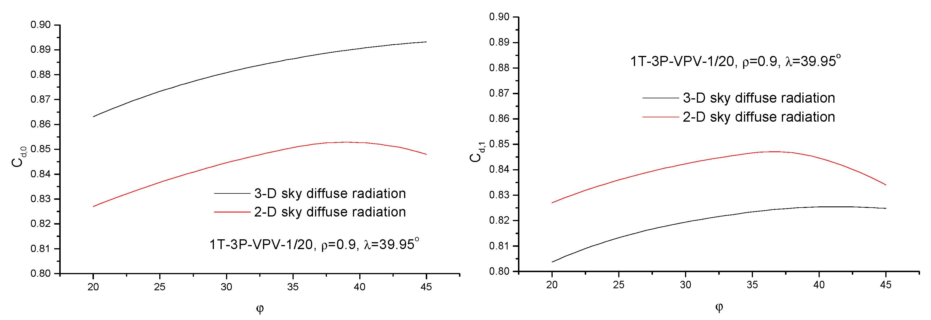
Figure 8 shows a comparison of C_d,0 and C_d,1 of 3P-VPV-1/20 calculated based on 2-D and 3-D sky diffuse radiation models. It shows that the 2-D model underestimates C_d,0 but overestimates C_d,1. This means that 2-D sky diffuse radiation can’t reasonably estimate the collectible sky diffuse radiation of a fixed inclined north-south V-trough. However, recent work of Tang et al. [28] indicates that the 2-D model can reasonably estimate sky diffuse radiation on solar cells of east-west CPV. This is because the directional intensity of sky diffuse radiation on the cross-section of a horizontal east-west CPV is really isotropic, but not for inclined north-south V-trough or CPCs, as explained in Appendix C.

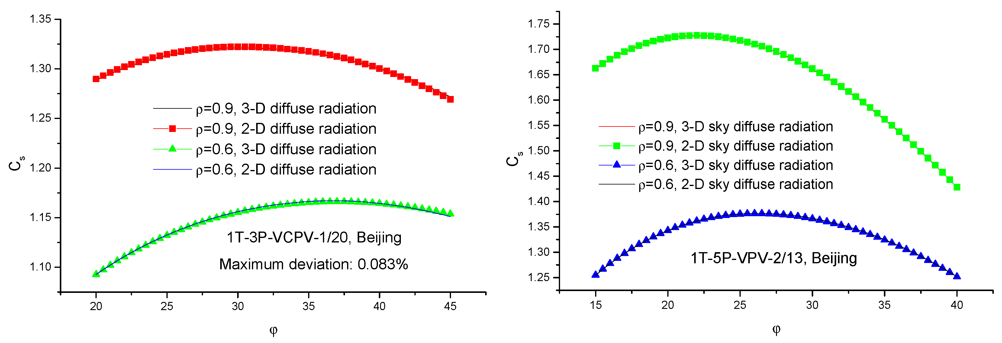
Comparisons of annual solar gain of 1T-MP-VPVs calculated based on 2-D and 3-D sky diffuse radiation are presented in Figure 9 in terms of C_s. It is found that the difference of annual solar gain calculated based on 2-D and 3-D sky diffuse radiation is less than 0.1%, indicating that 2-D sky diffuse radiation can reasonably predict the annual solar gain of MP-VPVs although it can’t predict the solar gain of fixed inclined north-south V-troughs. In the subsequent calculations, 3-D sky diffuse radiation is employed as 2-D sky diffuse radiation can’t predict the photovoltaic performance of linear concentrator-based PV systems [28].

4.2. Effects of Geometry of V-trough on the Performance of MP-VPV-k/θ_a

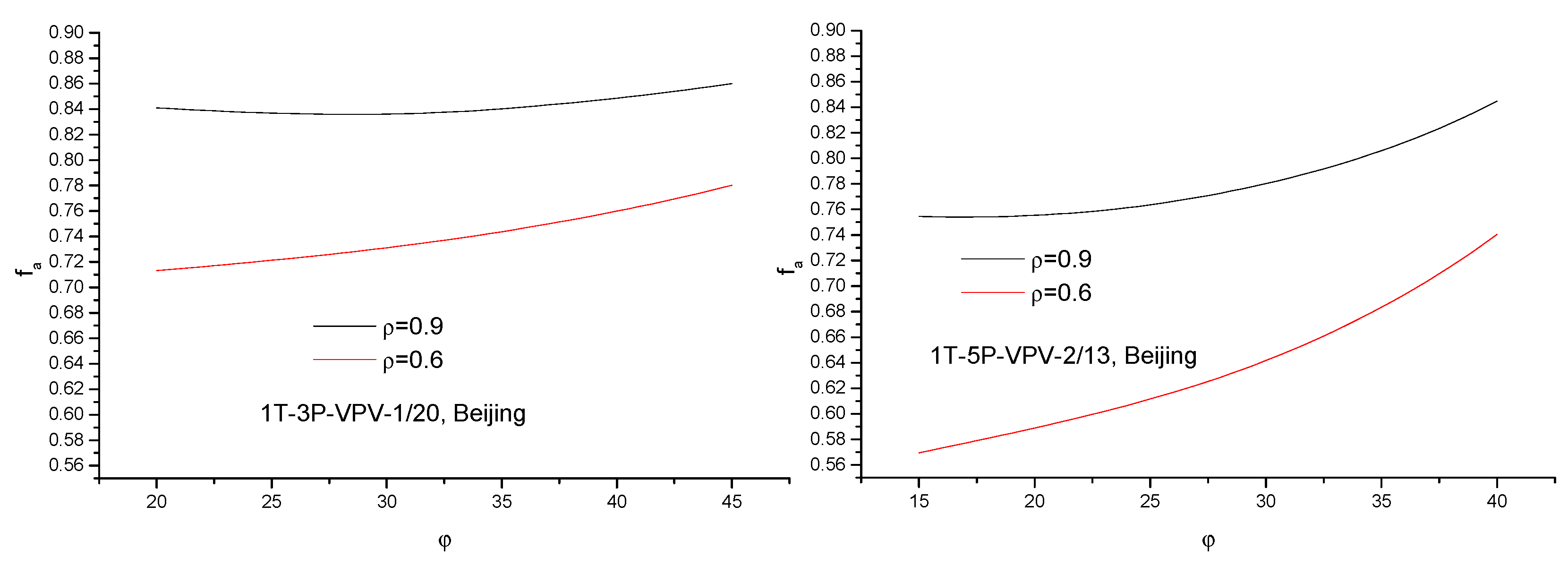
The analysis above shows that the annual power output of MP-VPV-k/${\theta }_a$ is sensitive to M and the geometry of VPVs at a site, therefore, given M, k and ${\theta }_a$, the performance of MP-VPV-k/${\theta }_a$ depends on $\phi$. As shown in Figure 10, the $f_a$ is highly dependent on $\rho$. For MP-VPVs with k = 2, the $f_a$ increases with the increase of $\phi$ as more radiation directly irradiates on the solar cells; whereas for MP-VPVs with k = 1 and high $\rho$, the $f_a$ is weakly sensitive to $\phi$ because, with the increase of $\phi$, more radiation directly irradiates on solar cells on the one hand, but in the other hand, more fraction of radiation incident on walls of the V-trough arrives on solar cells after more than one reflection.

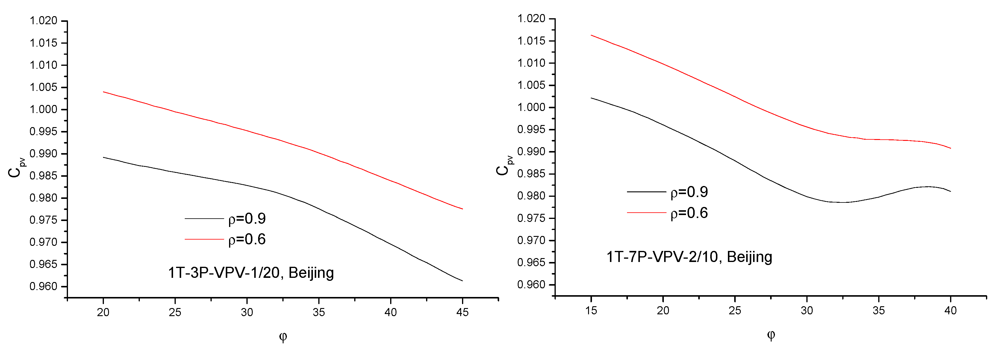
Figure 11 presents effects of $\phi$ on the photovoltaic efficiency of solar cells for radiation concentrated by MP-VPV-k/${\theta }_a$. It is seen that, for MP-VPV-k/${\theta }_a$ with k = 1, the C_pv decreases with the increase of $\phi$ as the IA of solar rays on solar cells also increases, thus the photovoltaic efficiency decreases; whereas for MP-VPV-k/${\theta }_a$ with k = 2, there is a swing because, with the increase of $\phi$, the IA on solar cells increases on the one hand, but in the other hand, more radiation directly irradiates on the solar cells. Therefore there is a trade-off between increased optical efficiency due to more radiation directly incident on the solar cells and decreased photovoltaic efficiency of the solar cells due to increased IA. Anyway, it is seen that C_pv is above 0.96 for 15° <$\phi$ < 40°, indicating that the electric loss of MP-VPV-k/${\theta }_a$ due to increased IA on solar cells after radiation concentration is insignificant.

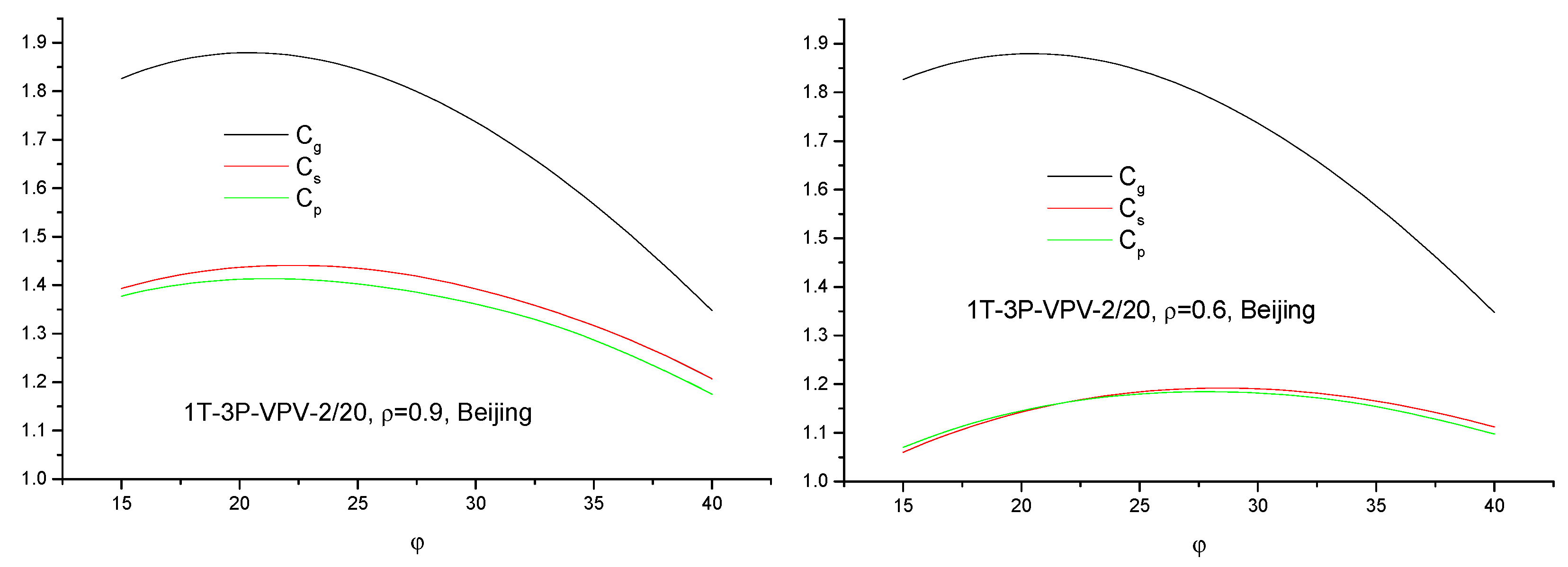
Effects of $\phi$ on the annual collectible radiation and electricity generation of MP-VPV-k/${\theta }_a$ are presented in Figure 12 and Figure 13. It is seen that C_s and C_p are sensitive to $\phi$, and ${\phi }_s$, the optimal $\phi$ for maximizing S_a is commonly larger than ${\phi }_p$, the optimal $\phi$ for maximizing P_a. It is also found that, as compared to similar multiple positions Sun-tracked PV panels, the increase factors of annual solar gain (C_s) and power output (C_p) of MP-VPV-k/${\theta }_a$ are similar but much lower than the geometric concentration since C_p = C_pvC_s and C_pv$\approx$1.

These results indicate that the power increase (C_p) of MP-VPV-k/${\theta }_a$ being much less than C_g is mainly attributed to the optical loss due to imperfect reflections, and the electric loss due to increased IA after radiation concentration is insignificant. Results shown in Figure 12 and Figure 13 indicate that a 3° deviation of $\phi$ from ${\phi }_p$ results in reduction of P_a less than 0.5%. The analysis above shows that, for a given MP-VPV-k/${\theta }_a$, an optimal $\phi$ for maximizing P_a can be found, hence different ${\theta }_a$ yields different ${\phi }_p$ thus different optimal geometry of MP-VPVs for maximizing P_a. As shown in Figure 14, given a Sun-tracking strategy (M), the maximum annual power output in terms of C_p,0, the ratio of P_a to P_a,0, is sensitive to ${\theta }_a$, hence an optimal ${\theta }_a$ for maximizing P_a of MP-VPV-k/${\theta }_a$ can be found. It is seen that, as compared to similar fixed south-facing PV panels, the annual power output increase C_p,0 of MP-VPV-k/${\theta }_a$ is even larger than C_g,p, the C_g of VPVs optimized for maximizing P_a, in sites with abundant solar resources such as Beijing, but in sites with poor solar resources such as Chongqing, C_p,0 is always less than C_g,p. This implies that MP-VPV-k/${\theta }_a$ is suitable to be used in sites with abundant solar resources. Calculations also indicate that 1° deviation of ${\theta }_a$ from the optimal value results in reduction of P_a less than 0.3%.

4.3. Optimal Design of MP-VPV-k/θ_a for Maximizing Annual Power Output

4.3.1. Optimal Design of 1T-MP-VPV-k/θ_a

In this case, the tilt angle of INSA is fixed yearly at $\lambda$. Hence, given M, $\rho$ and k, the P_a is dependent on ${\theta }_a$ and $\phi$, thus a set of optimal ${\theta }_a$ and $\phi$ for maximizing P_a in a site can be found by two-loop iterative calculations. As shown in

Table 1. Optimal design of 1T-3P-VPV-k/${\theta }_a$ for maximizing annual power output.

Site	ρ	1T-3P-VPV-1/${\mathit{\theta }}_{\mathit{a}}$						1T-3P-VPV-2/${\mathit{\theta }}_{\mathit{a}}$
		${\mathit{\theta }}_{\mathit{a}}$	${\mathit{\phi }}_{\mathit{g}}$	${\mathit{\phi }}_{\mathit{g}}$	Cg,p	Cp	Cp,0	${\mathit{\theta }}_{\mathit{a}}$	${\mathit{\phi }}_{\mathit{g}}$	${\mathit{\phi }}_{\mathit{p}}$	Cg,p	Cp	Cp,0
Beijing	0.9	20.4	29.5	28.6	1.569	1.298	1.624	19.8	20.4	21.3	1.888	1.414	1.766
	0.8	20.8	29.4	30.3	1.559	1.247	1.562	20.4	20.4	23.2	1.849	1.328	1.661
	0.7	21.4	29.3	31.6	1.542	1.198	1.503	21	20.3	25.2	1.797	1.252	1.568
	0.6	22	29.2	33.2	1.523	1.152	1.447	21.8	20.2	27.3	1.724	1.183	1.484
Shanghai	0.9	20	29.6	29	1.58	1.269	1.513	19.4	20.5	21.7	1.905	1.368	1.63
	0.8	20.4	29.5	30.6	1.569	1.22	1.455	20.2	20.4	23.8	1.852	1.286	1.534
	0.7	21	29.4	32.4	1.55	1.173	1.401	21	20.3	26	1.784	1.214	1.449
	0.6	21.4	29.3	34.5	1.532	1.13	1.349	21.4	20.2	28.3	1.719	1.15	1.373
Lhasa	0.9	21.8	29.3	28.1	1.534	1.311	1.716	21.4	20.2	21.1	1.818	1.427	1.865
	0.8	22.2	29.2	29.5	1.525	1.261	1.652	22	20.1	22.8	1.783	1.343	1.758
	0.7	22.6	29.1	30.8	1.514	1.214	1.591	22.6	20	24.8	1.736	1.267	1.662
	0.6	23.2	29	32.2	1.497	1.168	1.532	23.2	19.9	26.6	1.681	1.2	1.575
Chongqing	0.9	19	29.7	29.6	1.607	1.237	1.415	18.4	20.6	22	1.952	1.324	1.513
	0.8	19.4	29.7	31.8	1.594	1.189	1.36	19.4	20.5	24.6	1.879	1.244	1.423
	0.7	20.2	29.6	33.8	1.567	1.145	1.309	20.2	20.4	27.2	1.797	1.175	1.344
	0.6	21	29.4	36.2	1.534	1.104	1.262	20.8	20.3	29.6	1.712	1.116	1.276

, the optimal design of 1T-3P-VPV-k/${\theta }_a$ is dependent on $\rho$ and the climatic conditions in a site. For a given site, the optimal ${\theta }_a$ slightly increases with the decrease of $\rho$. It is seen that, for k = 1, the optimal ${\theta }_a$ varies from 20.5° to 22° as $\rho$ decreases from 0.9 to 0.6 except Lhasa (a site with extremely abundant solar resources) where it varies from 21.8° to 23.2° and Chongqing (a site poor in solar resources) where it varies from 19° to 21°; whereas for k = 2, the optimal ${\theta }_a$ is about 0.5° lower than that of similar 3P-VPV with k = 1.

Results in Table 1 show that, for $\rho$ > 0.8, ${\phi }_p$ is close to ${\phi }_g$, the optimal $\phi$ for maximizing C_g; whereas for $\rho$ < 0.8, ${\phi }_p$ is about 3–5° larger than ${\phi }_g$. As aforementioned, 1° deviation of ${\theta }_a$ from the optimal value and 2–3° deviation of $\phi$ from ${\phi }_p$ results in the reduction of P_a by less than 0.5%. Therefore, for 1T-3P-VPV-k/${\theta }_a$ (k = 1 and 2), ${\theta }_a$ = 21° as the optimal value is advisable except sites with extremely abundant solar resources where ${\theta }_a$ = 22° is recommended and sites poor in solar resources where ${\theta }_a$ = 20° is suggested.

Also, it is seen that, for ρ > 0.8, ${\phi }_p$ = ${\phi }_g$ is advisable, and for ρ < 0.8, ${\phi }_p$ = ${\phi }_g$ + 4° is recommended. Results listed Table 1 also indicate that, as compared to similar fixed PV panels, the annual power increase (C_p,0) of 3P-VPVs is higher than C_g,_p of an optimized V-trough in the sites with abundant solar resources for ρ > 0.8.

Optimal designs of 1T-5P-VPV-k/${\theta }_a$ are presented in

Table 2. Optimal designs of 1T-5P-VPV-k/${\theta }_a$ for maximizing annual power output.

Site	ρ	1T-5P-VPV-1/${\mathit{\theta }}_{\mathit{a}}$						1T-5P-VPV-2/${\mathit{\theta }}_{\mathit{a}}$
		${\mathit{\theta }}_{\mathit{a}}$	${\mathit{\phi }}_{\mathit{g}}$	${\mathit{\phi }}_{\mathit{p}}$	Cg,p	Cp	Cp,0	${\mathit{\theta }}_{\mathit{a}}$	${\mathit{\phi }}_{\mathit{g}}$	${\mathit{\phi }}_{\mathit{p}}$	Cg,p	Cp	Cp,0
Beijing	0.9	13.4	29.9	28.8	1.79	1.474	1.897	13	20.9	21	2.282	1.708	2.196
	0.8	13.8	30	29.6	1.775	1.405	1.81	13.4	20.9	22.2	2.25	1.59	2.046
	0.7	14	30	30.8	1.768	1.339	1.725	13.8	20.9	23.4	2.213	1.48	1.906
	0.6	14.4	30	32	1.751	1.274	1.643	14.4	20.9	24.8	2.156	1.377	1.776
Shanghai	0.9	13	29.6	28.8	1.806	1.428	1.739	13	20.9	21.2	2.282	1.633	1.987
	0.8	13.4	29.9	30.2	1.791	1.362	1.659	13.4	20.9	22.6	2.247	1.52	1.851
	0.7	13.8	30	31.6	1.774	1.298	1.581	13.8	20.9	24	2.206	1.416	1.725
	0.6	14	30	33	1.763	1.236	1.506	14.2	20.9	25.6	2.156	1.32	1.608
Lhasa	0.9	13.8	30	28.4	1.774	1.51	2.032	14	20.9	20.8	2.211	1.753	2.362
	0.8	14.2	30	29.2	1.76	1.44	1.941	14.2	20.9	22	2.196	1.635	2.204
	0.7	14.4	30	30.2	1.753	1.373	1.851	14.6	20.9	23.2	2.161	1.524	2.056
	0.6	14.8	30	31	1.739	1.306	1.763	14.8	20.9	24.6	2.133	1.421	1.918
Chongqing	0.9	12.8	29.9	29.2	1.814	1.375	1.596	12.6	20.9	21.4	2.311	1.551	1.8
	0.8	13	29.9	31	1.806	1.312	1.523	13	20.9	23	2.273	1.443	1.676
	0.7	13.4	29.9	32.8	1.786	1.251	1.452	13.4	20.9	24.8	2.223	1.345	1.562
	0.6	13.8	30	34.6	1.764	1.193	1.385	14	20.9	26.6	2.15	1.255	1.457

. It is seen that the optimal ${\theta }_a$ in this case for k = 1 and 2 are almost identical, and varies from about 13° to 14.5° as ρ decreases from 0.9 to 0.6, except at Lhasa where it varies from 13.8° to 14.8°. Therefore, ${\theta }_a$ = 13.5° is advisable as the optimal value except for Lhasa where ${\theta }_a$ = 14.5° is recommended. It is seen from Table 2 that for k = 1, ${\phi }_p$ is close to ${\phi }_g$, except at Chongqing in the case of $\rho$ = 0.6, hence ${\phi }_p$ = ${\phi }_g$ is recommended; whereas for k = 2, ${\phi }_p$ = ${\phi }_g$ and ${\phi }_p$ = ${\phi }_g$ + 3° are advisable for ρ > 0.8 and ρ < 0.8, respectively. Similarly, it is found that, C_p,0 is also larger than C_g,p in sites abundant in solar resources for ρ > 0.8.

Table 3. Optimal design of 1T-7P-VPV-k/${\theta }_a$ for maximizing annual power output.

Site	ρ	1T-7P-VPV-1/${\mathit{\theta }}_{\mathit{a}}$						1T-7P-VPV-2/${\mathit{\theta }}_{\mathit{a}}$
		${\mathit{\theta }}_{\mathit{a}}$	${\mathit{\phi }}_{\mathit{g}}$	${\mathit{\phi }}_{\mathit{p}}$	Cg,p	Cp	Cp,0	${\mathit{\theta }}_{\mathit{a}}$	${\mathit{\phi }}_{\mathit{g}}$	${\mathit{\phi }}_{\mathit{p}}$	Cg,p	Cp	Cp,0
Beijing	0.9	10	29.4	28.2	1.938	1.588	2.061	9.8	20.6	20.4	2.552	1.912	2.48
	0.8	10.2	29.4	29.2	1.929	1.507	1.957	10.2	20.7	21.4	2.513	1.768	2.296
	0.7	10.4	29.5	30.2	1.919	1.427	1.855	10.4	20.7	22.4	2.489	1.633	2.122
	0.6	10.8	29.6	31.2	1.899	1.349	1.754	10.8	20.8	23.4	2.444	1.506	1.959
Shanghai	0.9	9.8	29.3	28.8	1.948	1.53	1.874	9.8	20.6	20.6	2.552	1.816	2.224
	0.8	10	29.4	29.6	1.938	1.452	1.779	10.2	20.7	21.6	2.512	1.679	2.058
	0.7	10.2	29.4	30.8	1.928	1.376	1.686	10.4	20.7	22.8	2.486	1.552	1.902
	0.6	10.4	29.5	32.2	1.915	1.302	1.595	10.6	20.7	24.2	2.452	1.432	1.755
Lhasa	0.9	10.2	29.4	28	1.928	1.635	2.222	10.4	20.7	20.4	2.495	1.979	2.691
	0.8	10.4	29.5	28.8	1.919	1.552	2.11	10.6	20.7	21.2	2.477	1.834	2.494
	0.7	10.6	29.5	29.6	1.91	1.47	2.001	10.8	20.8	22	2.456	1.696	2.309
	0.6	10.8	29.6	30.4	1.9	1.39	1.892	11	20.8	23	2.431	1.566	2.132
Chongqing	0.9	9.6	29.2	28.6	1.958	1.464	1.707	9.6	20.6	20.8	2.572	1.709	1.993
	0.8	9.8	29.3	30.2	1.948	1.389	1.62	10	20.7	22.2	2.528	1.58	1.842
	0.7	10	29.4	32	1.934	1.318	1.536	10.2	20.7	23.6	2.495	1.461	1.703
	0.6	10.2	29.4	33.8	1.918	1.248	1.455	10.6	20.7	25.2	2.435	1.349	1.573

shows the optimal design of 1T-7P-VPV-k/${\theta }_a$. It is seen that, for k = 1, the optimal ${\theta }_a$ varies around 10° except for Lhasa where it varies around 10.5°, and ${\phi }_p$ varies around ${\phi }_g$ for 0.6 < ρ < 0.9; whereas for k = 2, the optimal ${\theta }_a$ varies around 10.5° and ${\phi }_p$ varies near ${\phi }_g$ for 0.6 < ρ < 0.9 except for Chongqing where ${\theta }_a$ = 10° and ${\phi }_p$ = ${\phi }_g$ + 3° is recommended. To be convenient for applications, optimal designs of MP-VPV-k/${\theta }_a$ recommended in this work are summarized in

Table 4. Recommended optimal design of MP-VPV-k/${\theta }_a$ for maximizing annual power output.

VPV	ρ	VPV-1/${\mathit{\theta }}_{\mathit{a}}$					VPV-2/${\mathit{\theta }}_{\mathit{a}}$
		${\mathit{\theta }}_{\mathit{a}}$	${\mathit{\phi }}_{\mathit{g}}$	${\mathit{\phi }}_{\mathit{p}}$	Cg,p	h	${\mathit{\theta }}_{\mathit{a}}$	${\mathit{\phi }}_{\mathit{g}}$	${\mathit{\phi }}_{\mathit{p}}$	Cg,p	h
1T-3P-	>0.8	21	29.4	29.5	1.554	1.053	21	20.3	20.5	1.836	2.311
	<0.8			33.5	1.547	0.908			24.5	1.807	1.859
1T-5P-	>0.8	13.5	29.6	29.5	1.787	1.494	13.5	20.9	21	2.246	3.362
	<0.8			29.5	1.787	1.494			24	2.227	2.887
1T-7P-	>0.8	10	29.4	29.5	1.939	1.782	10	20.7	21	2.533	4.135
	<0.8			29.5	1.939	1.782			24	2.508	3.548
3T-3P-	>0.8	20	29.6	29.5	1.581	1.102	20	20.4	20.5	1.86	2.432
	<0.8			32.5	1.576	0.988			24.5	1.852	1.963
3T-5P-	>0.8	13	29.9	30	1.806	1.505	13	20.9	21	2.282	3.459
	<0.8			30	1.806	1.505			23	2.273	3.129
3T-7P-	>0.8	9.5	29.2	29.5	1.964	1.83	10	20.7	21	2.533	4.136
	<0.8			29.5	1.964	1.83			24	2.508	3.548

.

4.3.2. Optimal Design of 3T-MP-VPV-k/θ_a

In this case, the tilt-angle of INSA is adjusted yearly four times at three tilts. Therefore, given M, ρ and k, the P_a is dependent on date (N) when a tilt-angle adjustment is made, tilt-angle adjustment ($\alpha$) from site latitude for each adjustment, ${\theta }_a$ and $\phi$, thus a set of optimal N, $\alpha$, ${\theta }_a$ and $\phi$ for maximizing P_a in a site can be found by multiple-loop iterative calculations. As seen from

Table 5. Optimal design of 3T-3P-VPV-1/${\theta }_a$ for maximizing annual power output.

Sites	ρ	N	$\mathit{\alpha }$	${\mathit{\theta }}_{\mathit{a}}$	${\mathit{\phi }}_{\mathit{p}}$	Cg,p	Cp	Cp,0	Pa	Cp,3T-1T	Pa,r
Beijing	0.9	22	24.8	19.2	29	1.602	1.322	1.727	1478.5	1.063	1477.6
	0.8	22	24.8	19.8	30.4	1.585	1.269	1.66	1421	1.063	1420.7
	0.7	22	25	20.4	31.8	1.567	1.219	1.595	1366	1.062	1365.6
	0.6	22	25	21	33.4	1.547	1.171	1.534	1313.6	1.06	1312
Shanghai	0.9	22	23	19	29.2	1.607	1.292	1.595	1096.8	1.054	1095.9
	0.8	22	23	19.6	30.8	1.59	1.241	1.533	1054.1	1.054	1053.7
	0.7	22	23.2	20.2	32.6	1.571	1.193	1.474	1013.6	1.053	1013.6
	0.6	22	23	20.6	34.2	1.554	1.148	1.418	975.1	1.051	974
Lhasa	0.9	22	25	20.4	28.6	1.569	1.341	1.823	2381.4	1.063	2380
	0.8	22	24.8	21	29.8	1.554	1.289	1.754	2290.6	1.061	2290.4
	0.7	22	24.6	21.4	31	1.543	1.238	1.687	2202.9	1.06	2201.8
	0.6	22	24.6	21.8	32.2	1.531	1.19	1.622	2118.4	1.059	2117.3
Chongqing	0.9	22	22	18.6	29.8	1.619	1.256	1.482	765	1.047	763.9
	0.8	22	22.4	19.2	31.8	1.6	1.207	1.424	735.4	1.047	734.5
	0.7	21	22.2	19.8	33.6	1.578	1.161	1.37	707.5	1.046	707.4
	0.6	21	22	20.2	35.8	1.557	1.119	1.32	681.4	1.045	680.6

and

Table 6. Optimal design of 3T-3P-VPV-2/${\theta }_a$ for maximizing annual power output.

Sites	ρ	N	$\mathit{\alpha }$	${\mathit{\theta }}_{\mathit{a}}$	${\mathit{\phi }}_{\mathit{p}}$	Cg,p	Cp	Cp,0	Pa	Cp,3T-1T	Pa,r
Beijing	0.9	22	24.2	18.8	21.4	1.935	1.449	1.891	1618.9	1.07	1615.7
	0.8	22	24.6	19.4	23.2	1.895	1.359	1.776	1520.8	1.069	1513.5
	0.7	22	24.8	20.4	25.2	1.824	1.278	1.673	1432.4	1.067	1432.1
	0.6	22	25	20.8	27.2	1.77	1.207	1.58	1353.3	1.065	1346.6
Shanghai	0.9	22	23.4	18.6	21.6	1.944	1.403	1.73	1189.6	1.061	1186.9
	0.8	22	23.2	19.4	23.6	1.891	1.317	1.626	1117.7	1.06	1111
	0.7	22	23.4	20	25.8	1.833	1.241	1.533	1053.8	1.058	1052.7
	0.6	22	23.2	20.6	28.2	1.756	1.174	1.45	997	1.056	989.4
Lhasa	0.9	22	25.2	20	21	1.879	1.471	1.998	2608.7	1.071	2605.6
	0.8	22	25.2	20.8	22.8	1.834	1.381	1.879	2454.3	1.069	2444.1
	0.7	22	25.2	21.4	24.6	1.788	1.301	1.773	2314.9	1.067	2314.1
	0.6	22	25.2	21.8	26.6	1.738	1.23	1.676	2189	1.064	2179.3
Chongqing	0.9	22	22.2	18	22	1.973	1.35	1.592	822	1.052	820.5
	0.8	22	22.2	18.8	24.4	1.911	1.258	1.496	772.3	1.051	766.5
	0.7	22	22.2	19.6	26.8	1.833	1.196	1.411	728.7	1.05	727.8
	0.6	22	22.6	20.4	29.4	1.735	1.134	1.338	690.8	1.048	684.4

, the optimal N is 21–22 days from equinoxes for all cases; whereas the optimal $\alpha$, strongly sensitive to climatic conditions in the site and slightly to $\rho$, M and k, varies from 22° to 25°. Calculations show that, for a given 3T-MP-VPV-k/${\theta }_a$, one day of N from the optimal value and 2° of $\alpha$ from its optimal value results in reduction of P_a less than 0.1%. Hence, N = 22 days and $\alpha$ = 23.5° are recommended as optimal N and $\alpha$, respectively. It is seen from Table 5 and Table 6 that, as compared to 1T-MP-VPVs, the annual power output of 3T-MP-VPVs is about 5% higher (see the columns of C_p,3T-1T) in sites with poor solar resources and 6% in sites with abundant solar resources.

Table 5 shows that the optimal ${\theta }_a$ of 3T-3P-VPV-1/${\theta }_a$ varies from 19° to 21° as ρ decreases from 0.9 to 0.6 except for Lhasa, where it varies from 20.4 to 21.8°_, and Chongqing, where it does so from 18.6 to 20.4°, hence, ${\theta }_a$ = 20° is recommend as the optimal value. It is also seen that the ${\phi }_p$ is about ${\phi }_g$ for ρ > 0.8 and ${\phi }_g$ + 3 for ρ < 0.8, thus ${\phi }_p$ = ${\phi }_g$ and ${\phi }_p$ = ${\phi }_g$ + 3 are recommended for ρ > 0.8 and ρ < 0.8, respectively. As seen from Table 5, the annual power output, P_a,r, estimated based on N = 22 days, $\alpha$ = 23.5° as well optimal ${\theta }_a$ and ${\phi }_p$ suggested in Table 4 are almost identical to P_a of optimal 3T-3P-VPV-1/${\theta }_a$ with the maximum deviation of less than 0.1%.

Optimal designs of 3T-3P-VPV-2/${\theta }_a$ are given in Table 6. It indicates that, except for Lhasa and Chongqing, the optimal ${\theta }_a$ varies from 18.6° to 21.2°, ${\phi }_p$ is about ${\phi }_g$ for ρ > 0.8 and ${\phi }_g$ + 4 for ρ < 0.8. Hence, ${\theta }_a$ = 20° as the optimal value is advisable, and ${\phi }_p$ = ${\phi }_g$ and ${\phi }_p$ = ${\phi }_g$ + 4 are recommended for ρ > 0.8 and ρ < 0.8, respectively. It is also seen that, the annual power output, P_a,r, calculated based on recommended optimal values of N, $\alpha$, ${\theta }_a$ and ${\phi }_p$ are almost identical to those (P_a) of optimal 3T-3P-VPV-2/${\theta }_a$.

To save space, optimal designs of 3T-5P-VPV- k/${\theta }_a$ and 3T-7P-VPV-k/${\theta }_a$ are not presented in details, and their recommended optimal designs are presented in Table 4. It is seen from Table 4 that, with the increase of M, the ${\theta }_a$ decreases, but C_g and h of VPVs optimized for maximizing P_a increase. For MP-VPVs with k = 1, the C_g,p is less than 2, and h < 1.83; whereas for k = 2, 1.8 < C_g,p < 2.53 and 1.8 < h < 4.1. In practical applications, one should select ${\theta }_a$ and M based on the requirement of C_g first, then determine ${\phi }_p$ based on ρ and ${\phi }_g$, which is close to 30° for k = 1 and 21° for k = 2 as 8° < ${\theta }_a$ < 25°. Considering the fact that V-trough with h > 2 is not practical, therefore, 5P-, and 7P-VPV-2/${\theta }_a$ are not advisable for applications.

5. Conclusions

Calculations and analysis show that the directional intensity of sky diffuse radiation on the cross-section of a linear concentrators is not isotropic except when the cross-section is parallel or perpendicular to the horizon, hence 2-D sky diffuse radiation can’t reasonably predict collectible sky diffuse radiation of fixed inclined north-south V-troughs, but can for MP-VPVs.

Analysis shows that, at a specific site, the annual collectible radiation and power output of MP-VPV-k/${\theta }_a$ is dependent on M and the geometry of VPVs. Calculations show that ${\phi }_s$, the optimal $\phi$ for maximizing S_a, is commonly larger than ${\phi }_p$, the optimal $\phi$ for maximizing P_a. It is also found that, as compared to similar multiple positions Sun-tracked PV panels, the increases of S_a and P_a of MP-VPV-k/${\theta }_a$ are similar but much lower than C_g. Analysis shows that the power increase factor, C_p, being much less than C_g is mainly attributed to the optical loss due to imperfect reflections, and the electric loss due to increased IA of solar rays on solar cells after radiation concentration is insignificant.

Results show that, the optimal design of 1T-MP-VPV-k/${\theta }_a$ for maximizing P_a is dependent on M, climatic conditions in sites and reflectivity of the side walls (ρ). The optimal ${\theta }_a$ is about 21°, 13.5° and 10° for 3P-, 5P- and 7P-VPVs (k = 1 and 2), respectively; whereas ${\phi }_p$ is about ${\phi }_g$ for ρ > 0.8 and about 3–4° larger than ${\phi }_g$ for ρ < 0.8. As compared to similar fixed south-facing PV panels, the increase of annual electricity from MP-VPV-k/${\theta }_a$ is even larger than the C_g,p of optimized MP-VPV-k/${\theta }_a$ for ρ > 0.8 in sites with abundant solar resources.

Calculations indicate that, for 3T-MP-VPV-k/${\theta }_a$, the optimal date (N) when tilt-angle adjustment is made is about 22 days from equinoxes, and the optimal tilt adjustment from site latitude (α) for each adjustment is about 23.5°. It is found that the optimal ${\theta }_a$ of 3T-MP-VPV-k/${\theta }_a$ is about 0.5° less than that of similar 1T-MP-VPV-k/${\theta }_a$, and ${\phi }_p$ is almost identical to that of similar 1T-MP-VPV-k/${\theta }_a$. As compared to similar 1T- MP-VPV-k/${\theta }_a$, the annual electricity generation from 3T-MP-VPV-k/${\theta }_a$ is about 5–7% higher.

In practical applications, one should select ${\theta }_a$ and M based on the requirement of C_g first, then determines ${\phi }_p$ based on ρ and ${\phi }_g$, which is about 30° for k = 1 and 21° for k = 2 as 8° < ${\theta }_a$ < 25°. However 5P-, and 7P-VPV-2/${\theta }_a$ are not advisable as the height of the V-trough is more than twice the width of the base.

References

- Xia, C.; Luo, H.; Tang, R.; Zhong, H. Solar thermal utilization in China. Renew. Energy 2004, 29, 1549–1556. [Google Scholar] [CrossRef]
- Tang, R.; Yang, Y. Nocturnal reverse flow in water-in-glass evacuated tube solar water heaters. Energy Convers. Manag. 2014, 80, 173–177. [Google Scholar] [CrossRef]
- Muhammad-Sukki, F.; Abu-Bakar, S.H.; Ramirez-Iniguez, R.; McMeekin, S.G.; Stewart, B.G.; Munir, A.B.; Yasin, S.H.M.; Rahim, R.A. Performance analysis of a mirror symmetrical dielectric totally internally reflecting concentrator for building integrated photovoltaic systems. Appl. Energy 2013, 111, 288–299. [Google Scholar] [Green Version]
- Nsengiyumva, W.; Chen, S.; Hu, L.; Chen, X. Recent advancements and challenges in Solar Tracking Systems (STS): A review. Renew. Sustain. Energy Rev. 2018, 81, 250–279. [Google Scholar] [CrossRef]
- Mallick, T.K.; Eames, P.C. Design and fabrication of low concentrating second generation PRIDE concentrator. Sol. Energy Mater. Sol. Cells 2007, 91, 597–608. [Google Scholar] [CrossRef]
- Mallick, T.K.; Eames, P.C.; Hyde, T.J.; Norton, B. The design and experimental characterization of an asymmetric compound parabolic photovoltaic concentrator for building façade integration in the UK. Sol. Energy 2004, 77, 319–327. [Google Scholar] [CrossRef]
- Mallick, T.K.; Eames, P.C.; Norton, B. Non-concentrating and asymmetric compound parabolic concentrating building façade integrated photovoltaic: An experimental comparison. Sol. Energy 2006, 80, 834–849. [Google Scholar] [CrossRef]
- Yousef, M.S.; Rahman, A.K.A.; Ookawara, S. Performance investigation of low—Concentration photovoltaic systems under hot and arid conditions: Experimental and numerical results. Energy Convers. Manag. 2016, 128, 82–94. [Google Scholar] [CrossRef]
- Su, Y.; Pei, G.; Saffa, B.R.; Huang, H. A novel lens-walled compound parabolic concentrator for photovoltaic applications. J. Sol. Energy Eng. 2012, 134, 021010. [Google Scholar] [CrossRef]
- Li, G.; Pei, G.; Su, Y.; Ji, J.; Saffa, B.R. Experiment and simulation study on the flux distribution of lens-walled compound parabolic concentrator compared with mirror compound parabolic concentrator. Energy 2013, 58, 398–403. [Google Scholar]
- Li, G.; Tang, J.; Tang, R. A note on design of dielectric compound parabolic concentrator. Sol. Energy 2018, 171, 500–507. [Google Scholar] [CrossRef]
- Li, G.; Tang, J.; Tang, R. A theoretical study on performance and design optimization of linear dielectric compound parabolic concentrating photovoltaic systems. Energies 2018, 11, 2454. [Google Scholar] [CrossRef]
- Yu, Y.; Liu, N.; Li, G.; Tang, R. Performance comparison of CPCs with and without exit angle restriction for concentrating radiation on solar cells. Appl. Energy 2015, 155, 284–293. [Google Scholar] [CrossRef]
- Baig, H.; Sarmah, N.; Chemisana, D.; Rosell, J.; Mallick, T.K. Enhancing performance of a linear dielectric based concentrating photovoltaic system using a reflective film along the edgy. Energy 2014, 73, 177–191. [Google Scholar] [CrossRef]
- Sangani, C.S.; Soanki, C.S. Experimental evaluation of V-trough (2 suns) PV concentrator system using commercial PV modules. Sol. Energy Mater. Sol. Cells 2007, 91, 453–459. [Google Scholar] [CrossRef]
- Solanki, C.S.; Sangani, C.S.; Gunasheka, D.; Antony, G. Enhanced heat dissipation of v-trough PV modules for better performance. Sol. Energy Mater. Sol. Cells 2008, 92, 1634–1638. [Google Scholar] [CrossRef]
- Vilela, O.C.; Fraidenraich, N.; Bione, J. Long term performance of water pumping systems driven by photovoltaic V-trough generators. In Proceedings of the ISES Solar World Congress 2003, Gotemborg, Sweden, 14–19 June 2003. [Google Scholar]
- Bione, J.; Vilela, O.C.; Fraidenraich, N. Comparison of the performance of PV water pumping systems driven by fixed, tracking and V-trough generators. Sol. Energy 2004, 76, 703–711. [Google Scholar] [CrossRef]
- Bione, J.; Vilela, O.C.; Fraidenraich, N. Simulation of grape culture irrigation with photovoltaic V-trough pumping systems. Renew. Energy 2004, 29, 1697–1705. [Google Scholar]
- Fraidenraich, N.; Vilela, O.C. Performance of solar systems with nonlinear behavior calculated by the utilizability method. Application to PV solar pumps. Sol. Energy 2000, 69, 131–137. [Google Scholar] [CrossRef]
- Huang, B.J.; Sun, F.S. Feasibility study of one axis three positions tracking solar PV with low concentration ratio reflector. Energy Convers. Manag. 2007, 48, 1273–1280. [Google Scholar] [CrossRef]
- Huang, B.J.; Ding, W.L.; Huang, Y.C. Long-term test of solar PV power generation using one-axis 3-position sun tracker. Sol. Energy 2011, 85, 1935–1944. [Google Scholar] [CrossRef]
- Gomez-Gila, F.J.; Wang, X.T.; Barnett, A. Energy production of photovoltaic systems: Fixed, tracking, and concentrating. Renew. Sustain. Energy Rev. 2012, 16, 306–313. [Google Scholar] [CrossRef]
- Zhong, H.; Li, G.; Tang, R.; Dong, W. Optical performance of inclined south-north axis three positions tracked solar panels. Energy 2011, 36, 1171–1179. [Google Scholar] [CrossRef]
- Tang, R.; Liu, X. Optical performance and design optimization of V-trough concentrators for photovoltaic applications. Sol. Energy 2011, 85, 2154–2166. [Google Scholar] [CrossRef]
- Rabl, A. Comparison of solar concentrators. Sol. Energy 1976, 18, 93–111. [Google Scholar] [CrossRef]
- Tang, R.; Wu, M.; Yu, Y.; Li, M. Optical performance of fixed east-west aligned CPCs used in China. Renew. Energy 2010, 35, 1837–1841. [Google Scholar] [CrossRef]
- Tang, J.; Yu, Y.; Tang, R. A three-dimensional radiation transfer model to evaluate performance of compound parabolic concentrator-based photovoltaic systems. Energies 2018, 11, 896. [Google Scholar] [CrossRef]
- Rabl, A. Active Solar Collectors and Their Applications; Oxford University Press: Oxford, UK, 1985. [Google Scholar]
- Li, W.; Pau, M.C.; Sellami, N.; Sweet, T.; Montecucco, A.; Siviter, J.; Baig, H. Six-parameter electrical model for photovoltaic cell/module with compound concentrator. Sol. Energy 2016, 137, 551–563. [Google Scholar] [CrossRef]
- Tang, R.; Wang, J. A note on multiple reflections of radiation within CPCs and its effect on calculations of energy collection. Renew. Energy 2013, 57, 490–496. [Google Scholar] [CrossRef]
- Chen, Z.Y. The Climatic Summarization of Yunnan; Weather Publishing House: Beijing, China, 2001. [Google Scholar]
- Collares-Pereira, M.; Rabl, A. The average distribution of solar radiation: Correlations between diffuse and hemispherical and between hourly and daily insolation values. Sol. Energy 1979, 22, 155–164. [Google Scholar] [CrossRef]
Figure 1.
Consecutive images of VPV-k/.
Figure 2.
Effects of on Cg of VPV-k/.
Figure 3.
Effect of θa on Cg and ϕg of VPV-k/θa optimized for maximizing Cg.
Figure 4.
Back view of 7P-VPV-k/.
Figure 5.
Radiation () directly irradiating on base of V-trough.
Figure 6.
Radiation “irradiating” on kth right image of base ().
Figure 7.
Vector of sky diffuse radiation from an element on the sky dome in the (x,y,z) coordinate system.
Figure 8.
Comparison of Cd,0 and Cd,1 of 1T-3P-VPV-1/20 calculated based on 2-D and 3-D sky diffuse radiation.
Figure 9.
Comparison of annual solar gain of 1T-MP-VPVs calculated by 2-D and 3-D sky diffuse radiation.
Figure 10.
Effects of on annual average optical efficiency of 1T-MP-VPVs.
Figure 11.
Effects of on photovoltaic efficiency of solar cells within 1T-MP-VPVs.
Figure 12.
Effects of on annual solar gain and power output of 1T-3P-VPV-2/20.
Figure 13.
The same as in Figure 12 but for 1T-7P-VPV-1/10.
Figure 14.
Effects of on maximum annual power output of 1T-3P-VPV-1/ in terms of Cp,0.