A Novel Photovoltaic Array Outlier Cleaning Algorithm Based on Sliding Standard Deviation Mutation


1
State Key Laboratory of Alternate Electrical Power System with Renewable Energy Sources, North China Electric Power University, Beijing 102206, China
2
School of Renewable Energy, North China Electric Power University, Beijing 102206, China
3
State Grid HeNan Electric Power Company Research Institute, Zhengzhou 450000, China
4
Beijing Advanced Innovation Center for Soft Matter Science and Engineering, Beijing University of Chemical Technology, Beijing 100029, China
*
Author to whom correspondence should be addressed.
Energies 2019, 12(22), 4316; https://doi.org/10.3390/en12224316
Submission received: 9 October 2019
/
Revised: 7 November 2019
/
Accepted: 11 November 2019
/
Published: 13 November 2019
(This article belongs to the Special Issue Photovoltaic Modules)
Abstract
:There is a large number of outliers in the operation data of photovoltaic (PV) array, which is caused by array abnormalities and faults, communication issues, sensor failure, and array shutdown during PV power plant operation. The outlier will reduce the accuracy of PV system performance analysis and modeling, and make it difficult for fault diagnosis of PV power plant. The conventional data cleaning method is affected by the outlier data distribution. In order to solve the above problems, this paper presents a method for identifying PV array outliers based on sliding standard deviation mutation. Considering the PV array output characteristics under actual environmental conditions, the distribution of array outliers is analyzed. Then, an outlier identification method is established based on sliding standard deviation calculation. This method can identify outliers by analyzing the degree of dispersion of the operational data. The verification part is illustrated by case study and algorithm comparison. In the case study, multiple sets of actual operating data of different inverters are cleaned, which is selected from a large grid-connected power station. The cleaning results illustrate the availability of the algorithm. Then, the comparison against the quantile-algorithm-based outlier identification method explains the effectiveness of the proposed algorithm.
1. Introduction
Rapid growth in photovoltaic (PV) capacity requires continuous improvement of smart operation and maintenance of PV systems. The smart operation and maintenance platform for PV systems include core functions such as performance analysis, state evaluation, fault diagnosis, and predictive maintenance [1]. The implementation of such functions depends on high-quality and reliable data. The actual operation of the PV system, however, produces an abundance of outliers due to data propagation signal noise, sensor failure, communication and measurement equipment failure, maximum power tracking abnormalities, array shutdown, and power limitation, among other issues [2]. Outliers can seriously affect the quality of the original data and affect the implementation of intelligent operation and maintenance functions [3]. Data cleaning is the basis of intelligent PV operation and is of great significance in practical engineering applications.
Many researchers have been exploring outlier identification and data cleaning in new energy power generation systems. The global probability statistical method and the intelligent clustering method are commonly used for these purposes. Chen et al. [4], for example, proposed a method for automatically cleaning corrupted and lost load curve data based on B-spline smoothing and kernel-based smoothing techniques. Wang et al. [5] proposed a Copula-based joint probability model for eliminating wind power curve outliers. This model can capture complex nonlinear multivariate relationships among parameters based on the univariate marginal distribution. Shen [6] used the change point grouping algorithm and the quartile algorithm to remove outliers in wind curves. Ye [7] et al. introduced an outlier identification methodology based on a probabilistic wind farm power curve and typical outlier distribution characteristics; this methodology combines the time-series power data and spatial correlation between adjacent wind farms and can identify outliers effectively. Such a method is based on the probability and statistics theory, and a statistical model can be established using historical sample data. In short, statistical methods require prior knowledge of statistical characteristics of outliers for direct application.
Zheng [8] proposed an empirical clustering method to calculate the outliers in a wind database via local outlier factor (LOF) algorithm, where outliers are then used to evaluate the clustering performance. Yesibudak [9] proposed three levels of outlier data detection methods based on wind power curves, including K-means clustering based on the Euclidean distance, contour coefficient evaluation, and a partition clustering method based on the Mahalanobis distance. Schlechtingen et al. [10] compared fuzzy logic, neural network, and nearest neighbor models for data mining of wind turbine power curves. Three models were tested under different wind speed and temperature conditions, then were compared by the respective average absolute error, root mean square error, and average absolute percentage of the data samples. Intelligent methods have been widely used, however they have two main shortcomings. First, it is difficult to obtain sample data in the training process and the generalization ability of intelligent methods is difficult to be applied in the case of large fluctuations of PV output [11]. Second, the physical meaning of the results for intelligent clustering algorithm is difficult to explain [12].
Scholars have attempted to mitigate the above disadvantages by combining intelligent clustering methods with probabilistic methods. Zhao Y. [13] proposed a data-driven outlier elimination method, which combined four-dimensional and the density-based clustering methods. Sparse outliers are first eliminated by the quartile method, then a spatial noise clustering method based on density noise is applied to eliminate outliers in the stack.
Considering the random fluctuation characteristic of PV power output, some researchers have studied the outlier identification and data cleaning of PV power systems. Zhang et al. [14] proposed a method for the data cleaning of radiation data. He used the short-circuit current Isc as a self-reference parameter to obtain statistical distributions based on different performance descriptors with a confidence level of 0.99. The relationship between Isc and irradiance is good in linearity, but Isc cannot be obtained in the actual operation process. Yu [15] proposed a least-squares-based data cleaning method for PV historical operation data. However, this method did not consider the output characteristics of the photovoltaic array so that the distortion of the distributed parameters caused by the outliers cannot be eliminated. There are clear-cut relationships among the PV system output, electrical parameter distribution, and the external environment [16,17]. Such relationships can be exploited to optimize the PV array data cleaning design [18].
Considering the distribution characteristics of PV array outliers, this paper proposes an algorithm for PV array outlier identification based on sliding standard deviation mutation. In this study, the irradiance and power data are collected by a SCADA system. The raw data are grouped according to the irradiation. Then, the variance of the data in different groups is used to determine the outlier. The rest of this paper is organized as follows. Section 2 outlines the establishment of the curve between PV irradiation quantity and power as well as the source distribution characteristics of PV array outliers during actual system operation. Section 3 defines the sliding standard deviation mutation algorithm and its step-wise solution process. Section 4 compares the data cleaning performance of this algorithm with the quantile algorithm. Section 5 provides a brief summary and conclusion.
2. PV Array Electrical Characteristics and the Outlier Distribution
2.1. PV Array Electrical Characteristics
The relationship between the PV array power, current, voltage, and external environmental parameters must be established to further investigate the actual operational data distribution of the array. The current I and voltage V under the theoretical condition of PV module can be calculated by Formulas (1)–(2) [19]. The theoretical output power calculation formula of the PV array is shown in Formulas (3)–(5) [20].
Gref = 1000 W/m2 is the reference solar radiation intensity, Tref = 25 °C is the reference temperature, e is the base of the natural logarithm (about 2.71828), the compensation coefficients a, b, c are constant, Voc-ref and Vm-ref are the open circuit voltage and the optimal operating point voltage of the PV module under standard conditions, and Isc-ref and Im-ref are the short-circuit current and the optimal operating point current of the PV module under standard conditions. For a PV array, the theoretical output power is calculated as follows:
where G is the irradiance, is the solar cell transmittance of the outer layer, is the conversion efficiency of the solar cell, is the value of thermal coefficient of max power for crystalline silicon and , A is the surface area of the PV module receiving surface, and Tc is the operating temperature of the solar cell.
The cell operating temperature is not easy to get in actual cases, so TNOCT is adopted for calculating the cell conversion efficiency:
where TNOCT is the temperature at normal operating cell temperature (NOCT) conditions and GNOCT is the irradiance at NOCT conditions.
The output power of the module is:
where Ta is the ambient temperature.
According to Formulas (1)–(5), combined with the Simulink model, the theoretical curves of the operating current I, and the irradiance G, the power P and the irradiance G are established, as shown in Figure 1.
As shown in Figure 1, theoretically, the two curves of the PV array’s operating current I and irradiance G, the PV array’s output power P and irradiance G approximate a linear relationship. The relationship between PV array operational data and environmental variables is the foundation for analyzing the source of outliers.
2.2. Source and Distribution of the Outlier
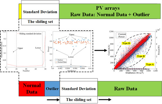
The data collected from the actual operation of the PV array usually contain a large number of outliers. The causes of outliers in photovoltaic systems mainly include hardware failure, signal noise, photovoltaic power limitation, and so on [21,22]. Moreover, outliers generated by various causes show different characteristics in the electrical parameter curve. Based on the relationship between irradiance and output power, this paper analyzes the distribution characteristics of abnormal data and classifies the types of outliers. Figure 2a shows the PV array monitoring structure. Figure 2b shows the distribution and source of PV array outliers.
According to Figure 2, the relationship between the distribution of outliers and the source is as follows.
- 1
- Type A outliers are “bottom stacked outliers”. They are typically caused by a fault or abnormality that cannot be recovered immediately. These faults or anomalies cause the system to continuously generate outliers within a short period of time. The feature of type A outlier is that the output of the array remains zero while the irradiance is normal, and such outliers are caused by:
- (1)
- PV arrays or inverter failure;
- (2)
- Communication equipment or sensor failure;
- (3)
- Power unit shutdown.
In these cases, the output power measurement of the PV array is zero or close to zero. The distribution features are stacked at the bottom of the curve.
- 2
- B-type outliers are “around scattered outliers”. They are irregular scattering points near the power curve and are typically caused by faults or abnormalities that can be recovered in a short period of time, including:
- (1)
- Communication equipment or sensor signal propagation noise;
- (2)
- Random volatility of external inputs;
- (3)
- The inaccuracy of MPPT (maximum power point tracking).
The outlier caused by random factors fluctuate randomly around normal data; such outliers will be randomly distributed outside the boundaries of the output curve.
3. Sliding Standard Deviation Mutation Algorithm
3.1. Sliding Standard Deviation Mutation Algorithm Principle
In this paper, as mentioned above, the distribution characteristics of PV array outliers form the basis for determining outliers. When outliers emerge in the operational data, data characteristics such as the rate of change, mean value, variance, standard deviation, and variance rate will change, so the appropriate mutation index can be selected to accurately identify the outliers. The standard deviation can objectively and accurately reflect the degree of dispersion of the dataset and is most commonly used in probability statistics as a measure of the degree of statistical distribution [23]. Therefore, the standard deviation is chosen as a suitable indicator of mutation. However, the standard deviation between different groups of the same sample is discrete, which has a negative impact on the accuracy of the final evaluation results. Therefore, this paper introduces the sliding standard deviation. The advantage of the sliding standard deviation is that the design of the sliding window can be used to maintain the continuity of the standard deviation of the data between different groups and to increase the sensitivity of the mutation index [24].
The known set U is divided into m mutually independent subsets Y, where U= {Y1, Y2, ⋯, Ym}, m is the number of Y. Let X = {Xs, X1} be the target set. Xs represents the data subset with normal array power generation performance, X 1 represents the data subset with abnormal array power generation performance, and X meets Xs ∩ X1= ∅, Xs ∪ X1=U.
Set the sliding set to Zj = {(x1, y1), (x2, y2), ⋯, (xa, ya)}, where Zj indicates that the sliding set in a subset slides to the jth position, j= 1, 2 ⋯ n-a+1, i=1, 2…n. a is the total number of data points in the sliding set and 1 < a < n, where n is the total number of subset data points. The known subset Ym= {(x1,y1), (x2,y2), ⋯, (xn,yn)∣yi<yi-1, i∈(2,n)}, where x represents irradiance, y represents power, and n is the total number of subset data points. The sliding standard deviation within the group is calculated as follows [25]:
where σm,j is the jth standard deviation value in the subset Ym, a is the total number of data points in the sliding set, and μ is the average value of yi in the sliding set.
Then, the change-point analysis is made for the calculation result of the sliding standard deviation, and the standard deviation threshold H is set based on the analysis result:
where i represents the ith point in the subset Ym within the standard deviation threshold, imin is the first point, and imax is the last point. After getting the normal point within the threshold of each subset, there is:
where Xs is the normal data subset of the sample set U and X1 is the outlier subset of the sample set U.
3.2. Algorithm Steps in Detail
The measured irradiance and power data of a PV array are chosen to illustrate the steps of the sliding standard deviation algorithm in detail. Figure 3 shows the flow chart of the algorithm.
The detailed steps of the algorithm are as follows (the solar irradiance and power of PV array have been normalized).
- (1)
- Select raw data U. The selected data contain the measured solar irradiance and power data of the PV array of one year.
- (2)
- Divide U into subsets Ym. The maximum value of irradiance data in the sample data is 1100 W/m2 and the minimum value is 0 W/m2, so the range of irradiance is 0–1100 W/m2. The data are divided into several subsets according to the irradiance interval. According to the rule of the algorithm, the data of each subset must meet the requirement of minimum data size. This restriction can be adjusted according to the total amount of sample data. The minimum data size of the selected data is 60. Therefore, when the data points in the subset are less than 60, the subset is merged with the previous subset until the data size requirements are met. The irradiance interval is set as T = 10 W/m2, and the sample data are divided into 110 subsets Ym that meet the rule. The calculation process of each subset is similar, so the 90th subset is taken as an example, of which the irradiance range is 900–910 W/m2.
- (3)
- Sort the subset data in descending order. There are 110 power points in the 90th subset, and the data points are arranged in descending order to satisfy yi<yi-1, i∈(2,110). The 90th subset is Y90 = {(x1,y1), (x2,y2),⋯,(x110,y110)}, where xi is the irradiance and yi is the power of the ith data point (xi, yi).
- (4)
- Calculate the sliding standard deviation. Set the data capacity of the sliding to a = 30. The subset data are brought into the sliding set Zj where j = 1, 2, ⋯, 81, as shown in Figure 4. Calculate sliding standard deviations of 81 sliding sets. The 81 sliding standard deviations and other specific data are shown in Table 1.
- (5)
- Set the threshold to identify outliers. First, set the threshold based on the distribution of sliding standard deviations. Calculate the deviation of 110 subsets Ym and divide the 110-subset deviation data into 11 groups according to the irradiance interval (100 W/m2). Then, number the 11 groups by Roman numerals (I for the 0–100 W/m2 irradiance interval, II for the 100–200 W/m2 irradiance interval, and so on).
The box diagram is shown in Figure 5. The statistical distribution of the 110 subsets’ sliding standard deviations shows that most of the normal values are concentrated between 0.015 and 0.025.
After the threshold is set to 0.02, the sliding standard deviation curve of the subset Y90 is shown in Figure 6a. The curve on the left side of the 20th value and the right side of the 73rd value is significantly upturned with no tendency to stabilize. The steady trend in the middle of the curve indicates that the sliding standard deviation of this part is similar and that the data fluctuation range is small, which are the normal data. By combining the threshold and formula (7), the 20th data point of the subset Y90 and the 103th data point are determined as the mutation points. Therefore, the first 19 data points (“Upper” area in Figure 6a) and last 8 data points (“Lower” area in Figure 6a) are identified as the outliers. The cleaning result is shown in Figure 6b.
4. Verification
In order to further verify the effectiveness of the outlier cleaning method proposed in this paper, the operational data of a PV array combiner box are chosen for the verification. The operational data are selected from a large grid-connected photovoltaic power station in China. All irradiance data and power data have been normalized.
4.1. Case Study
The total installed capacity of the grid-connected PV power station is 39.3 MW, and there are 74 centralized inverters installed, each of which is connected to six array combiner boxes. Sixteen PV branches are connected to each array combiner, and each branch has 16 PV modules connected in series. The model number of the module is CEC6-72-300P. The actual operation data of the two array combiner boxes in 2017 are selected as cleaning sample data (numbered 4A, 37A). The data resolution is 10 min.
Threshold settings directly influence data cleaning results, and different threshold setting schemes alter the data cleaning results. The threshold setting range is presented in Section 3. The data of the 37A array combiner box are taken as an example here to illustrate the cleaning effect of the sliding standard deviation mutation algorithm of different threshold settings. There is a linear relationship between power and irradiance, so the linear correlation coefficient is introduced as the evaluation index. The calculation results are shown in Table 2.
As shown in Table 2, the threshold setting affects the data deletion rate and linear correlation coefficient of the cleaning result. Within the designed threshold range, the linear correlation coefficient is stable above 99% and increases slightly as the threshold decreases. At the same time, the data deletion rate markedly increases as the threshold decreases. A smaller threshold setting causes a denser normal data distribution (Figure 8) and a larger threshold setting causes a more dispersed normal data distribution.
The threshold settings need to be adjusted to the actual application scenario. For example, for the modeling a PV system, the data must be prioritized over a smaller threshold. In this case, the data threshold range for 37A can be set to 0–0.01 to delete some of the discrete, correct data for higher quality and for more densely distributed normal data. In this case study, we aimed at prevent misidentification to the greatest extent possible by analyzing the threshold settings. Table 3 and Figure 8 together show that a smaller threshold setting results in a slight increase in the linear correlation, but the corresponding data deletion amount significantly increases to the point that certain normal points are incorrectly identified as outliers. A larger threshold setting results in less data deletion, and the smaller the linear correlation coefficient, but more outliers are not recognized. The optimal threshold setting range for the 37A data is 0.02 to 0.025. Under the same principle, the optimal threshold setting range for the other two sets of data is 0.02–0.025.
Two arrays of data of 4A and 37A are cleaned by the proposed method, and thresholds of the two sets of data are all set to 0.02. The data cleaning results are shown in Figure 9. The outliers of 4A and 37A’s data can been effectively identified by the algorithm. The data marked in red in Figure 9 are identified as normal data, which are close to the theoretical PV power curve. The results of the two groups also prove that the bottom-curve stacked and around-curve scattered outliers are effectively identified by the proposed algorithm, which make it feasible and effective for data cleaning in large grid-connected PV arrays.
4.2. Comparison with Other Algorithms
In order to illustrate the performance of the proposed method, it is compared with the quantile method, which is the most common used in data cleaning. In this section, the quantile is set to quartile. The original operation data of 4A and 37A array in the above example are used as data samples for the quantile method and the sliding standard deviation mutation algorithm. Two kinds of methods are used to clean the sample data under different outlier distributions. Then, the cleaning effect, data deletion rate, and linear correlation coefficient are compared.
Three kinds of data conditions (outlier accumulation at the bottom, outlier around the top, and normal outlier distribution) are designed to assess the cleaning effect of the two methods. The cleaning results under different outlier distributions are shown in Figure 10, Figure 11 and Figure 12.
Figure 10, Figure 11 and Figure 12 show that in the case of bottom outlier accumulation and outlier around the top, the data identified as normal data by the quartile algorithm are offset to the accumulation side of the outlier due to the distribution of outliers. Some data are misjudged, which means some normal data are identified as outliers and some outliers are identified as normal data. The sliding standard deviation algorithm proposed in the paper has not been affected by the outlier distribution, which means that the algorithm can still classify the outliers from the operation data.
To analyze the performance of the proposed method, the raw operation data of the 4A, 37A, and another array numbered 17B is cleaned by the quartile method and the sliding standard deviation mutation algorithm, respectively.
Figure 13 shows the data cleaning results for 37A by the two methods. Both methods can identify bottom-stacked outliers, overall. The normal data identified by the quartile method are shifted downwards. The outlier in 37A is stacked in the lower part of the scatter, which influences the quartile method’s cleaning effect, resulting in a deviation of normal data recognition. The sliding standard deviation algorithm will not be affected by the distribution of outliers.
Table 3 shows the cleaning results by the two methods. The two methods show different cleaning results of the outlier around the normal data. The two methods’ linear correlation coefficient of the cleaned data can reach 99%. The data deletion rate of the quartile method for three arrays is 45.43%, 37.24%, and 32.14%, respectively, which is much larger than the 16.38%, 19.87%, and 12.96% data deletion rates of the sliding standard deviation mutation algorithm. Figure 10, Figure 11, Figure 12 and Figure 13 show that the quartile method identifies some normal data as outliers, so the quartile method has a higher normal data loss rate than the proposed method.
In summary, the data cleaning method based on the sliding standard deviation mutation algorithm can effectively identify bottom-stacked and around-curve scatter data in the array power-irradiance curve of different PV arrays. Although the outliers distort the distribution of the data, the proposed method can still effectively identify the outliers.
5. Conclusions
In order to effectively clean the outlier existing in the PV array, this paper presents the cleaning method based on the sliding standard deviation. The main work of the thesis includes: The distribution characteristics and sources of outliers in the actual operating data of PV arrays are analyzed and summarized. A method based on sliding standard deviation mutation is proposed for identifying PV array outliers. In the case study, the different actual operational data are selected as the cleaning sample. The results prove the availability of the algorithm, and the performance comparison with the quartile algorithm shows the effectiveness of the proposed algorithm. Based on the above works, the highlights of the paper can be summarized as follows:
- (1)
- The typical source and distribution features of PV array outliers are revealed. This study finds that the outliers of PV arrays can be sorted into two categories (bottom-stacked data and around-curve scatter data), and then summarizes the source and distribution of these two types outliers.
- (2)
- The linear relationship between PV array operational data and environmental variables is used as the foundation of the cleaning method. The proposed method is consistent with the output characteristic of PV array, which can improve the recognition rate. The cleaning results are consistent with the theoretical relationship between irradiance and output power.
- (3)
- The outlier data distribution will affect the effect of classical data cleaning algorithm and lead to misidentification. In this paper, it is found that the classical quantile method will be affected by different distributions of the outlier, and such influence will lead to misidentification of the outliers and reduce the accuracy. The method of this paper can avoid the negative effects of outlier distribution by the algorithm design of sliding groups.
The proposed method can be used to preprocess the original operational data of the PV array. By cleaning out irrelevant outliers, high-quality data samples are provided for subsequent work of the operation and maintenance of the power plant.
Author Contributions
Conceptualization, A.H.; methodology, A.H.; software, A.H. and Q.S.; investigation, A.H., Q.S., H.L., and Z.T.; data curation, H.L. and N.Z.; writing—original draft preparation, A.H. and H.Z.; supervision, H.Z.
Funding
This research was funded by the Research Funds from State Grid Corporation of China “SGHADK00PJJS1800072”.
Acknowledgments
The authors would like to acknowledge the financial support of the Research Funds from State Grid Corporation of China “SGHADK00PJJS1800072”.
Conflicts of Interest
The authors declare no conflict of interest.
Nomenclature
| G | Irradiance (W/m2) |
| I | Current (A) |
| V | Voltage (V) |
| P | Power (W) |
| T | Temperature (°C) |
| e | The base of the natural logarithm |
| a, b, c | Constant |
| A | Surface area of the PV module receiving surface (m2) |
| Cell conversion efficiency | |
| Solar cell transmittance of the outer layer | |
| Isc | Short-circuit current (A) |
| Isc-ref | Short-circuit current under standard conditions (A) |
| Im-ref | Optimal operating point current under standard conditions (A) |
| Vm-ref | Optimal operating point voltage under standard conditions (V) |
| Voc-ref | Reference open-circuit voltage (V) |
| Iref | Reference current (A) |
| Vref | Reference voltage (V) |
| Gref | Reference irradiance (W/m2) |
| Tref | Reference temperature (°C) |
| Conversion efficiency at reference temperature conditions | |
| Thermal coefficient of max power for crystalline silicon | |
| Tc | Operating temperature of the solar cell (°C) |
| Ta | Ambient temperature (°C) |
| GNOCT | Irradiance at normal operating cell temperature conditions (W/m2) |
| TNOCT | Temperature at normal operating cell temperature conditions (°C) |
References
- Zhao, X.; Wang, Z. Technology, cost, economic performance of distributed photovoltaic industry in China. Renew. Sustain. Energy Rev. 2019, 110, 53–64. [Google Scholar]
- Vikrant, S.; Chandel, S.S. Performance and degradation analysis for long term reliability of solar photovoltaic systems: A review. Renew. Sustain. Energy Rev. 2013, 27, 753–767. [Google Scholar]
- Sotiris, N.K.; Theocharis, T. Assessment of the safe operation and maintenance of photovoltaic systems. Energy 2015, 93, 1633–1638. [Google Scholar]
- Chen, J.; Li, W.; Lau, A.; Cao, J.; Wang, K. Automated load curve data cleaning in power systems. IEEE Trans. Smart Grid 2010, 1, 213–221. [Google Scholar] [CrossRef]
- Wang, Y.; Infield, D.G.; Stephen, B.; Galloway, S.J. Copula-based model for wind turbine power curve outlier rejection. Wind Energy 2010, 17, 1677–1688. [Google Scholar] [CrossRef]
- Shen, X.; Fu, X.; Zhou, C. A combined algorithm for cleaning abnormal data of wind turbine power curve based on change point grouping algorithm and quartile algorithm. IEEE Trans. Sustain. Energy 2018, 10, 46–54. [Google Scholar] [CrossRef]
- Ye, X.; Lu, Z.; Qiao, Y.; Min, Y.; O’Malley, M. Identification and correction of outliers in wind farm time series power data. IEEE Trans. Power Syst. 2016, 31, 4197–4205. [Google Scholar] [CrossRef]
- Zheng, L.; Hu, W.; Min, Y. Raw wind data preprocessing: A data-mining approach. IEEE Trans. Sustain. Energy 2015, 6, 11–19. [Google Scholar] [CrossRef]
- Yesilbudak, M. Partitional clustering-based outlier detection for power curve optimization of wind turbines. In Proceedings of the 2016 IEEE International Conference on Renewable Energy Research and Applications (ICRERA), Birmingham, UK, 20–23 November 2016. [Google Scholar]
- Schlechtingen, M.; Santos, I.F.; Achiche, S. Using data-mining approaches for wind turbine power curve monitoring: A comparative study. IEEE Trans. Sustain. Energy 2013, 4, 671–679. [Google Scholar] [CrossRef]
- Ji, F.; Cai, X.; Wang, J. Wind power correlation analysis based on hybrid copula. Autom. Electr. Power Syst. 2014, 38, 1–5, 32. [Google Scholar]
- Long, H.; Sang, L.; Wu, Z.; Gu, W. Image-based Abnormal Data Detection and Cleaning Algorithm via Wind Power Curve. IEEE Trans. Sustain. Energy 2019, 1, 1. [Google Scholar] [CrossRef]
- Zhao, Y.; Ye, L.; Wang, W.; Sun, H.; Tang, Y.; Ju, Y. Data-driven correction approach to refine power curve of wind farm under wind curtailment. IEEE Trans. Sustain. Energy 2017, 9, 95–105. [Google Scholar] [CrossRef]
- Zhang, J.; Zhang, S.; Liang, J.; Tian, B.; Hou, Z.; Liu, B.Z. Photovoltaic generation data cleaning method based on approximately periodic time series. In Proceedings of the 2017 International Conference on Environmental and Energy Engineering (IC3E 2017), Suzhou, China, 22–24 March 2017. [Google Scholar]
- Yu, L.; Wang, H.; Che, J.; Lu, J.; Zheng, X. Outliers screening for photovoltaic electric power based on the least square method. In Proceedings of the 2016 Chinese Control and Decision Conference, Yinchuan, China, 28–30 May 2016. [Google Scholar]
- Kumar, R.; Sinha, S.K.; Pandey, K. Effect of temperature, irradiation, humidity and wind on ideal/double diode PV system performance. In Proceedings of the 2016 IEEE 1st International Conference on Power Electronics, Intelligent Control and Energy Systems (ICPEICES), Delhi, India, 4–6 July 2016. [Google Scholar]
- Bengir, A.S.M.; Mohammad, A.C.; Shameem, A.; Mohammod, A.K. Prediction of solar irradiation and performance evaluation of grid connected solar 80 KWp PV plant in Bangladesh. Energy Rep. 2019, 5, 714–722. [Google Scholar]
- Gong, Y.; Lu, Z.; Qiao, Y.; Wang, Q.; Cao, X. Copula theory based machine identification algorithm of high proportion of outliers in photovoltaic power data. Autom. Electr. Power Syst. 2016, 40, 16–22. [Google Scholar]
- Zhang, X.L.; Liu, Q.H.; Li, B.; Ma, H.M. Analysis of output characteristics of photovoltaic system. Adv. Mater. Res. 2012, 512–515, 17–22. [Google Scholar] [CrossRef]
- Skoplaki, E.; Palyvos, J.A. On the temperature dependence of photovoltaic module electrical performance: A review of efficiency/power correlations. Sol. Energy 2009, 83, 614–624. [Google Scholar] [CrossRef]
- Asma, T.L.; Afef, B.B.A.; Ilhem, S.B. Fault detection and monitoring systems for photovoltaic installations: A review. Renew. Sustain. Energy Rev. 2018, 82, 2680–2692. [Google Scholar]
- Wen, C.; Kaile, Z.; Shanlin, Y.; Cheng, W. Data quality of electricity consumption data in a smart grid environment. Renew. Sustain. Energy Rev. 2017, 75, 98–105. [Google Scholar]
- Rajiv, K.; Rashmi, G.; Le, H.S.; Sudan, J.; Raghvendra, K. Boosting performance of power quality event identification with KL Divergence measure and standard deviation. Measurement 2018, 126, 134–142. [Google Scholar]
- He, Z.; Chen, Y.; Shang, Z.; Li, C.; Li, L.; Xu, M. A novel wind speed forecasting model based on moving window and multi-objective particle swarm optimization algorithm. Appl. Math. Model. 2019, 76, 717–740. [Google Scholar] [CrossRef]
- Lou, J.; Xu, J.; Lu, H.; Qu, Z.; Li, S.; Liu, R. Wind turbine data-cleaning algorithm based on power curve. Autom. Electr. Power Syst. 2016, 40, 116–121. [Google Scholar]
Figure 1.
Output characteristic of photovoltaic (PV) module.

Figure 2.
PV array monitoring structure and source of outlier: (a) PV array monitoring structure; (b) the distribution and source of PV array outliers.
Figure 2.
PV array monitoring structure and source of outlier: (a) PV array monitoring structure; (b) the distribution and source of PV array outliers.


Figure 3.
Sliding standard deviation mutation algorithm flow chart.

Figure 4.
Sliding set diagram.

Figure 5.
Box diagram of 110 subsets’ sliding standard deviations.

Figure 6.
Cleaning result: (a) Curve of sliding standard deviation of the 90th subset; (b) cleaning result of 90th subset.
Figure 6.
Cleaning result: (a) Curve of sliding standard deviation of the 90th subset; (b) cleaning result of 90th subset.

Figure 7.
PV array data cleaning results.

Figure 8.
Data cleaning results of different thresholds. (a)The cleaning results from 2D perspective; (b) The cleaning results from 3D perspective.
Figure 8.
Data cleaning results of different thresholds. (a)The cleaning results from 2D perspective; (b) The cleaning results from 3D perspective.

Figure 9.
Cleaning results of two arrays: (a) Cleaning result of 4A; (b) cleaning result of 37A.

Figure 10.
The cleaning result of outlier accumulation at the bottom: (a) The cleaning result of the quantile method; (b) the cleaning result of the proposed method.
Figure 10.
The cleaning result of outlier accumulation at the bottom: (a) The cleaning result of the quantile method; (b) the cleaning result of the proposed method.

Figure 11.
The cleaning result of outlier around the top: (a) The cleaning result of the quantile method; (b) the cleaning result of the proposed method.
Figure 11.
The cleaning result of outlier around the top: (a) The cleaning result of the quantile method; (b) the cleaning result of the proposed method.

Figure 12.
The cleaning result of two kinds of normal data distribution: (a–b) The cleaning result of the quantile method; (c–d) the cleaning result of the proposed method.
Figure 12.
The cleaning result of two kinds of normal data distribution: (a–b) The cleaning result of the quantile method; (c–d) the cleaning result of the proposed method.

Figure 13.
Cleaning results of two algorithms for 37A data: (a) Quantile method; (b) the proposed method.
Figure 13.
Cleaning results of two algorithms for 37A data: (a) Quantile method; (b) the proposed method.


Table 1.
The 90th subset’s sliding standard deviations and other data.
| Sliding Set | Date | Power (W) | Ambient Temperature (°C) | Irradiance (W/m2) | Module Temperature (°C) | Normalized Power | Sliding Standard Deviation |
|---|---|---|---|---|---|---|---|
| Z1 | 17/4/24 11:39 | 497,520.1 | 21.15 | 909.99 | 40.71 | 0.816 | 0.023 |
| Z2 | 17/6/25 13:39 | 444,015.9 | 29.69 | 909.97 | 46.69 | 0.728 | 0.021 |
| ⋮ | ⋮ | ⋮ | ⋮ | ⋮ | ⋮ | ⋮ | |
| Z80 | 17/5/16 10:49 | 459,500 | 26.35 | 902.87 | 47.36 | 0.754 | 0.185 |
| Z81 | 17/5/28 12:20 | 459,062.6 | 34.87 | 902.73 | 54.34 | 0.753 | 0.221 |
Table 2.
Data cleaning results of different threshold.
| Threshold Value | Raw Data Volume | Residual Data Volume | Data Deletion Rate | Linearly Dependent Coefficient |
|---|---|---|---|---|
| 0 | 22,151 | 14,336 | 35.28% | 99.78% |
| 0.01 | 22,151 | 17,605 | 20.52% | 99.69% |
| 0.015 | 22,151 | 18,604 | 16.01% | 99.65% |
| 0.02 | 22,151 | 19,281 | 12.96% | 99.62% |
| 0.025 | 22,151 | 19,590 | 11.56% | 99.60% |
| 0.03 | 22,151 | 19,984 | 9.78% | 99.42% |
| 0.04 | 22,151 | 20,697 | 6.56% | 99.25% |
Table 3.
Data cleaning results of two different algorithms.
| Raw Data | Linear Correlation Coefficient Before Cleaning | Method | Data Deletion Rate | Linear Correlation Coefficient after Cleaning |
|---|---|---|---|---|
| 4A | 95.46% | Quantile algorithm | 45.43% | 99.81% |
| Proposed algorithm | 16.38% | 99.46% | ||
| 17B | 94.48% | Quantile algorithm | 37.24% | 99.75% |
| Proposed algorithm | 19.87% | 99.56% | ||
| 37A | 96.60% | Quantile algorithm | 32.14% | 99.71% |
| Proposed algorithm | 12.96% | 99.62% |
© 2019 by the authors. Licensee MDPI, Basel, Switzerland. This article is an open access article distributed under the terms and conditions of the Creative Commons Attribution (CC BY) license (http://creativecommons.org/licenses/by/4.0/).
Share and Cite
MDPI and ACS Style
Hu, A.; Sun, Q.; Liu, H.; Zhou, N.; Tan, Z.; Zhu, H. A Novel Photovoltaic Array Outlier Cleaning Algorithm Based on Sliding Standard Deviation Mutation. Energies 2019, 12, 4316. https://doi.org/10.3390/en12224316
AMA Style
Hu A, Sun Q, Liu H, Zhou N, Tan Z, Zhu H. A Novel Photovoltaic Array Outlier Cleaning Algorithm Based on Sliding Standard Deviation Mutation. Energies. 2019; 12(22):4316. https://doi.org/10.3390/en12224316
Chicago/Turabian StyleHu, Aoyu, Qian Sun, Hao Liu, Ning Zhou, Zhan’ao Tan, and Honglu Zhu. 2019. "A Novel Photovoltaic Array Outlier Cleaning Algorithm Based on Sliding Standard Deviation Mutation" Energies 12, no. 22: 4316. https://doi.org/10.3390/en12224316
Note that from the first issue of 2016, this journal uses article numbers instead of page numbers. See further details here.