Rotor Eddy Current Loss Calculation of a 2DoF Direct-Drive Induction Motor

Abstract

A two-degree-of-freedom direct-drive induction motor (2DoFDDIM), whose solid rotor is coated with a copper layer, is capable of linear, rotary, and helical motions and has widespread applications. For solid-rotor motors, the calculation and analysis of rotor total eddy current loss (TECL) are crucial in studying the factors causing such a loss and possible loss reduction methods. In this study, a new nonlinear analytical method considering the saturation of the rotor core is proposed to solve the fundamental magnetic field. The new method divides the time period into segments. The magnetic field distribution at any time is obtained using Maxwell equations. The eddy current losses in the copper layer and rotor core caused by the fundamental magnetic field are calculated. The surface eddy current losses in the copper layer and rotor core caused by harmonics are calculated using a 2D analytical method. TECL is determined by the sum of eddy current and surface eddy current losses. Coefficients are utilized to consider eddy, saturation, and end-region effects when calculating the rotor core TECL. The new method is verified using 3D FEM, and the results show the proposed method has higher accuracy than the original method. The errors of the rotor core and copper layer TECLs are less than $6\%$ and $7.3\%$, respectively.

1. Introduction

A two-degree-of-freedom direct-drive induction motor (2DoFDDIM) [1,2,3,4] that produces rotary, linear, and helical motions has widespread applications in special industrial products, such as industrial robot arms, drill presses, and carving machines. A copper-coated solid rotor is applied to 2DoFDDIM to improve the motor output torque. This solid-rotor induction motor has a simple structure, high reliability, high mechanical strength, and low maintenance cost. However, it has inherent disadvantages, such as large rotor eddy current loss that leads to a serious temperature increase, which considerably affects the safety of operation and service life of motors. Thus, analysis and calculation of rotor eddy current loss are crucial.

The eddy current during solid-rotor induction motor operation is induced by fundamental and high-harmonic magnetic fields. Studies on the literature [5,6] used a 3D-space harmonic analytical model to investigate the air gap flux and secondary losses of a single-side linear induction motor with a solid and laminated back iron. The model considered skin, end, and edge effects. In reference [7], a 2D analytical method was established to compute the magnetic field distribution, eddy current, and steady-state performance of solid-rotor induction motors. In references [8,9], an analytical model based on Maxwell’s equations was proposed to calculate the surface eddy current losses. In another study [10], the surface eddy losses in the solid rotor of an induction motor were computed using a 2D analysis method and the Poynting theorem. However, the influence of rotor core saturation, which is an important factor, was disregarded in the above-mentioned analytical methods. Thus, this study proposes a new analytical method that considers the saturation effect of the rotor core to calculate the rotor eddy current loss. This consideration improves the accuracy of loss calculation.

In this study, a 2DoFDDIM is transformed into two single-degree-of-freedom motors, wherein the coupling effect is disregarded [11,12]. The rotary part is selected as a research object to calculate the rotor loss. The rotor total eddy current loss (TECL) consists of TECLs in the copper layer and rotor core. TECL in the copper layer includes eddy current loss caused by the fundamental field and surface eddy current loss caused by harmonic magnetic fields. The eddy current loss in the copper layer (ECLCL) is computed using an original linear analytical method and a new nonlinear analytical method that considers the nonlinearity of the rotor core. The surface eddy current losses in the copper layer (SECLCL) are computed using a 2D analytical method. TECL in the copper layer is determined by the sum of ECLCL and SECLCL. The eddy current loss and surface eddy current losses in the rotor core (ECLRC and SECLRC, respectively) are calculated using the new method and a 2D analytical method, respectively, and various coefficients are utilized to consider eddy, saturation, and end-region effects. The corrected analysis results are compared with those derived by the 3D finite element method (FEM), and the results show that the errors of the rotor core and copper layer TECLs are less than $6\%$ and $7.3\%$, respectively. The accuracy of the new nonlinear analysis method is verified.

2. Structure and Parameters

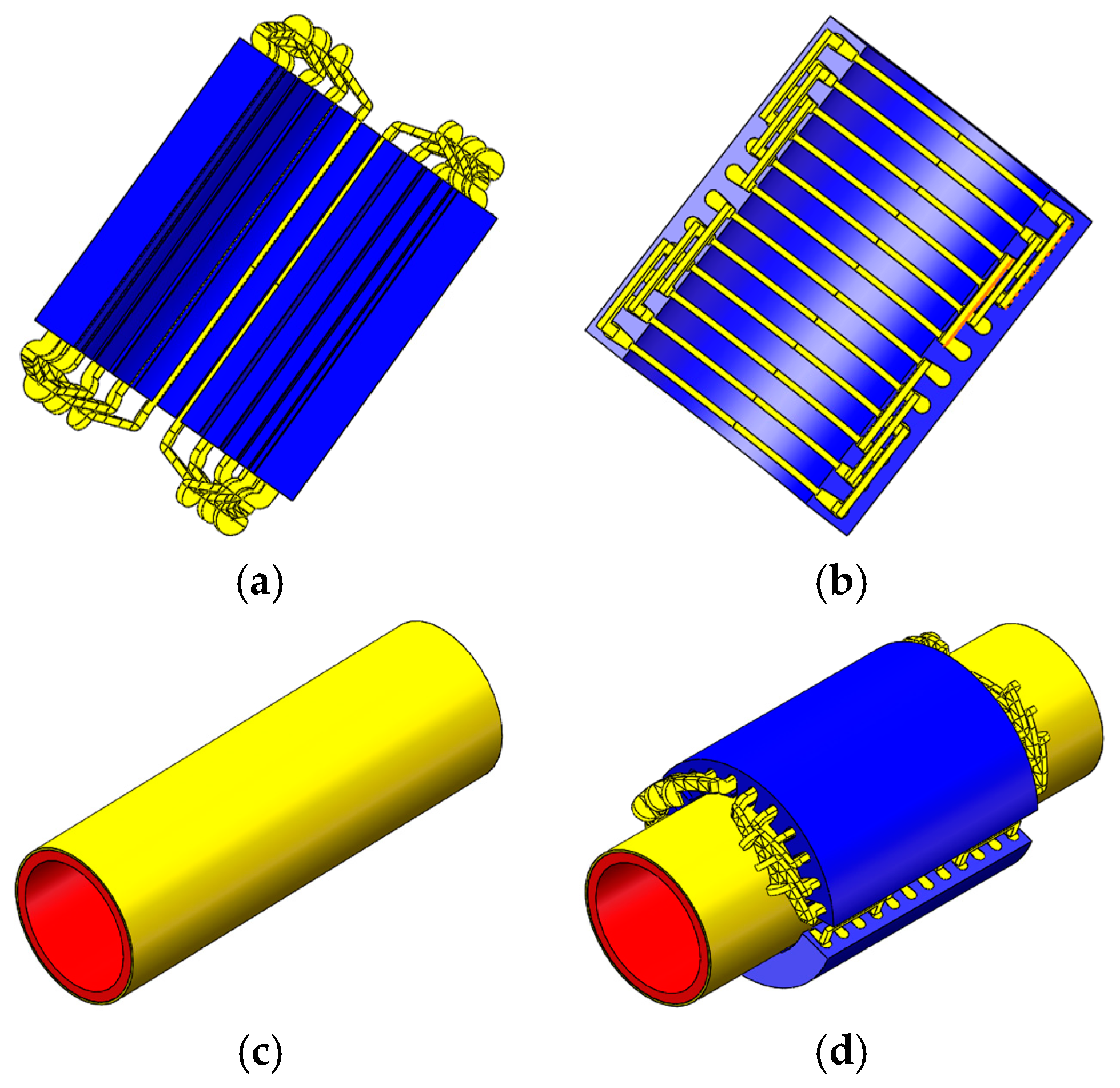
The 2DoFDDIM consists of two arc-shaped stators in the rotary and linear parts and a solid rotor coated with a copper layer, as shown in Figure 1.

The 2DoFDDIM can be transformed into two independent arc-shape linear induction motors if the coupling effect is ignored [2]. The rotary part is selected as the study object, and the main parameters are listed in

Table 1. Main parameters of the rotary part.

Item	Parameter
rated voltage	220 V (Y)
stator outer diameter	155 mm
stator inter diameter	98 mm
stator axial length	156 mm
slot number	12
phase	3
pole pair	2
thickness of air gap	1 mm
thickness of copper layer	1.5 mm
frequency	50 Hz

.

3. Rotor Calculation

The rotor TECL consists of the copper layer and rotor core TECLs, which are induced by fundamental and high-harmonic magnetic fields. Therefore, rotor TECL $P_r$ can be obtained as

$$\{\begin{array}{c}{P}_r=P_{Cu}{+P}_{Fe}\\ P_{Cu}=P_{Cu-eddy}{+P}_{Cuv}\\ P_{Fe}=P_{Fe-eddy}{+P}_{Fev}\end{array}$$

(1)

where $P_{Cu}$ and $P_{Fe}$ are TECLs in the copper layer and rotor core, respectively; $P_{Cu-eddy}$ and $P_{Fe-eddy}$ are eddy current losses in the copper layer and rotor core (ECLCL and ECLRC) caused by the fundamental magnetic field, respectively; $P_{Cuv}$ and $P_{Fev}$ are surface eddy current loss in the copper layer and rotor core (SECLCL and SECLRC) caused by harmonics, respectively.

3.1. Linear Analytical Method of ECLCL and ECLRC

3.1.1. Magnetic Field Analysis

The following assumptions are proposed to simplify the magnetic field analysis.

(1)

The curvature effect is disregarded. The rotor and stator are expanded into a semi-infinite flat model [13].

(2)

The phenomenon wherein the no-load speed exceeds the synchronous speed caused by the longitudinal edge effect is disregarded [14]. The synchronous speed is $n_1={60f}_1/p.$

(3)

The primary core has infinite permeability, and the conductivity is zero.

(4)

The end, hysteresis, and saturation effects are ignored. The rotor material is isotropic, and permeability and conductivity are constant.

(5)

The displacement current and influence of asymmetric three-phase current are ignored. The inducted current in the rotor only includes the z-component.

(6)

Each field includes a fundamental component, and the time variations of each field are sinusoidal.

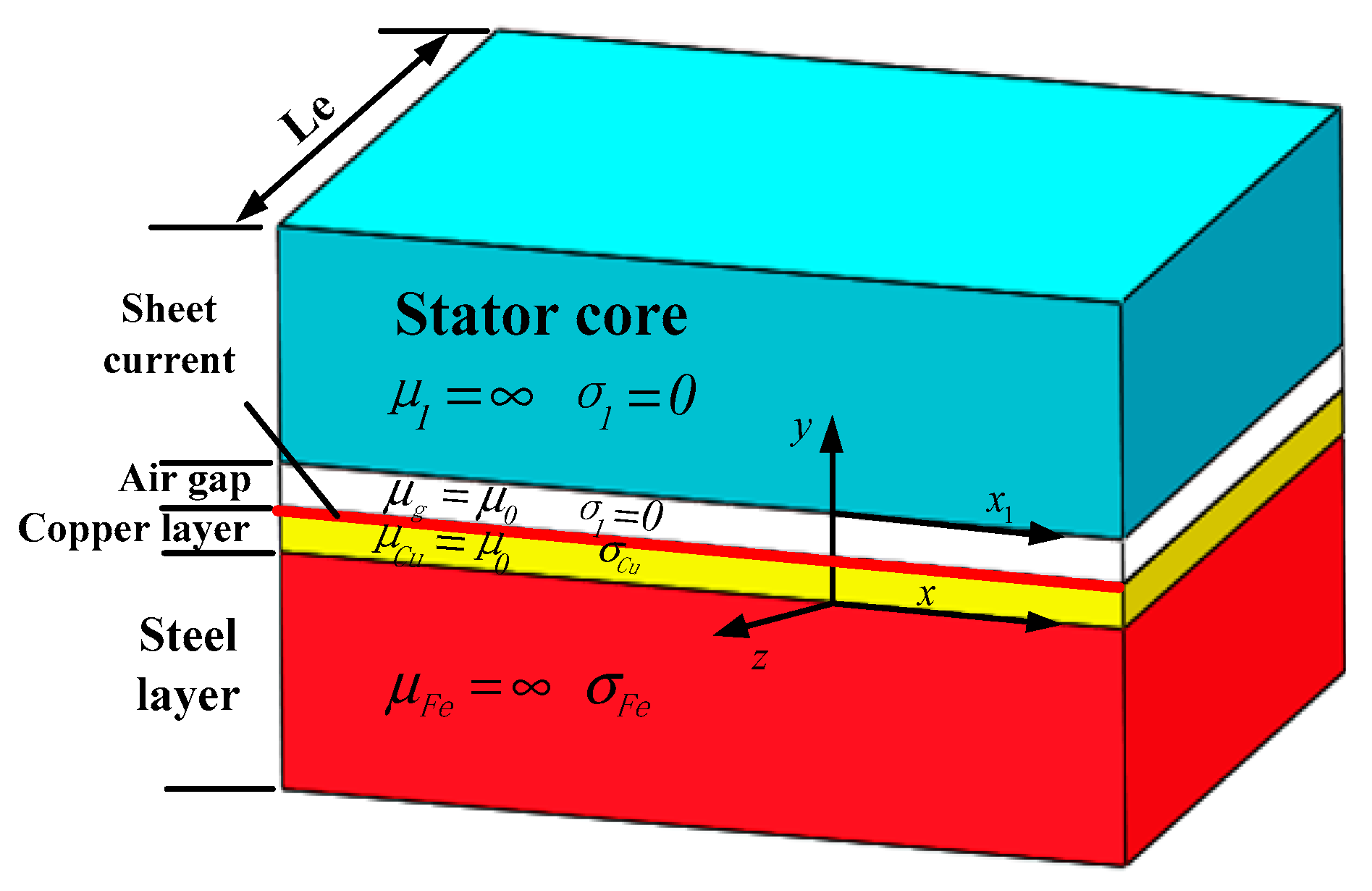
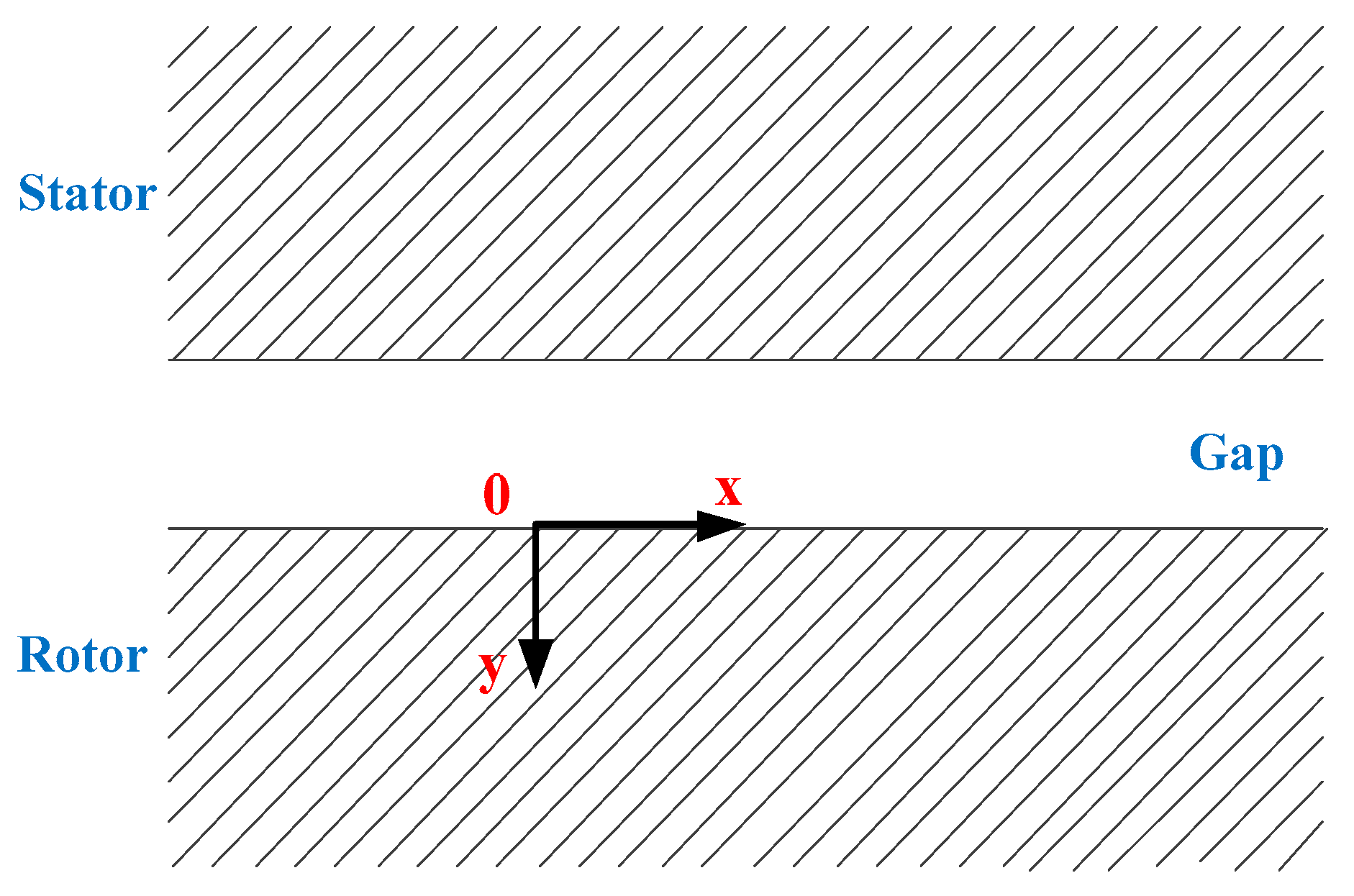
Two sets of the coordinate system are established to analyze the magnetic field distributions in the rotary part of the motor. Figure 2 shows an expanded plate model of the rotary part [15]. One set of the rectangular coordinate system (x, y, z) is fixed on the rotor, and another set (x₁, y, z) is fixed on the stator, in which the origins of the coordinates are taken at the center of the rotor. Here, x, y, and z express the circumferential, radial, and axial directions of the motor, respectively. The relationship between x₁ and x is ${\omega }_1{t-ax}_1{ = s\omega }_{1}t-ax$, where s indicates the slip, ${\omega }_1$ denotes the primary angular frequency, t is time, $a = \pi /\tau$, and $\tau$ is the pole pitch.

The stator winding current is equivalent to the sheet current at the junction of the stator and air gap, as shown in Figure 2. Sheet current density $\dot{{\mathit{J}}_{sz}}$ is sinusoidal and moves with a synchronous speed along the x-axis. The axial amplitude of $\dot{{\mathit{J}}_{sz}}$ is constant, and $\dot{{\mathit{J}}_{sz}}$ can be represented as a Fourier series with periodic 2L_e as follows [16]:

$$\dot{{\mathit{J}}_{sz}}{\displaystyle \sum }_n\frac{4}{\pi }{J}_0{e}^{j\left({\omega }_1{t-ax}_1\right)}\frac{1}{n}\sin \frac{n\pi }{L_e}z$$

(2)

where ${\sum }_n={\sum }_{n = 1,3,5,\cdots }$, $J_0=\sqrt{2}{m}_1{K}_{dp}{N}_1{I}_1/p\tau$ refers to the magnitude of the stator surface current density, $m_1$ is the number of the phases, K_dp represents the coefficient of fundamental winding, N₁ indicates the armature winding number, I₁ denotes the root mean square (RMS) of the stator phase current, $m_1$ is the number of the phases; $-L_e/2\le z\le L_e/2$, and L_e is the stator axial length.

The current density only has the z-component according to Assumption (5), i.e., $\dot{J}=\overrightarrow{k}{J}_z$, $J_x{=J}_y=0$. Thus, the vector magnetic potential is $\dot{A}=\overrightarrow{k}{A}_z$, $A_x{=A}_y=0$. The magnetic field differential equations of the air gap, rotor copper layer, and rotor core are as follows:

$$\frac{{\partial }^2\dot{{\mathit{A}}_{gz}}}{\partial x_1^2}+\frac{{\partial }^2\dot{{\mathit{A}}_{gz}}}{\partial y^2}+\frac{{\partial }^2\dot{{\mathit{A}}_{gz}}}{\partial z^2}=0$$

(3)

$$\frac{\partial \dot{{\mathit{A}}_{cz}}}{\partial x^2}+\frac{\partial \dot{{\mathit{A}}_{cz}}}{\partial y^2}+\frac{\partial \dot{{\mathit{A}}_{cz}}}{\partial z^2}{=js\omega }_1{\mu }_{Cu}{\sigma }_{Cu}\dot{{\mathit{A}}_{cz}}$$

(4)

$$\frac{\partial \dot{{\mathit{A}}_{iz}}}{\partial x^2}+\frac{\partial \dot{{\mathit{A}}_{iz}}}{\partial y^2}+\frac{\partial \dot{{\mathit{A}}_{iz}}}{\partial z^2}{=js\omega }_1{\mu }_{Fe}{\sigma }_{Fe}\dot{{\mathit{A}}_{iz}}$$

(5)

where $\dot{{\mathit{A}}_{gz}}$, $\dot{{\mathit{A}}_{cz}}$, and $\dot{{\mathit{A}}_{iz}}$ indicate the axial components of the vector magnetic potential of the air gap, rotor copper layer, and rotor core, respectively. Equations (1) to (4) are solved according to the boundary condition $\dot{{\mathit{A}}_{iz}}|{ }_{y=-\infty }=0$, and the vector magnetic potentials are obtained as follows:

$$\dot{{\mathit{A}}_{gz}}={\displaystyle \sum }_n{C}_{gn}{(\mathrm{ch}\lambda }_n{y+D}_n{\mathrm{sh}\lambda }_n{y)e}^{{j(\omega }_1{t-ax}_1)}\frac{1}{n}\sin \frac{n\pi }{L_e}z$$

(6)

$$\dot{{\mathit{A}}_{gz}}={\displaystyle \sum }_n{C}_{gn}{(\mathrm{ch}\lambda }_n{y+D}_n{\mathrm{sh}\lambda }_n{y)e}^{{j(\omega }_1{t-ax}_1)}\frac{1}{n}\sin \frac{n\pi }{L_e}z$$

(7)

$$\dot{{\mathit{A}}_{iz}}={\displaystyle \sum }_n{C}_{in}{e}^{{\alpha }_{n}y}{e}^{{j(s\omega }_{1}t-ax)}\frac{1}{n}\sin \frac{n\pi }{L_e}z$$

(8)

where ${\lambda }_v={[{\alpha }^2+{\left(n\pi /L_e\right)}^2]}^{\frac{1}{2}}$, ${\alpha }_{cn}={\left[{\lambda }_n^2{+js\omega }_1{\mu }_{Cu}{\sigma }_{Cu}\right]}^{\frac{1}{2}}$, and ${\alpha }_n={\left[{\lambda }^2{+js\omega }_1{\mu }_{Fe}{\sigma }_{Fe}\right]}^{\frac{1}{2}}$. C_gn, D_n, C_cn, D_cn and C_2n are undetermined coefficients.

The following boundary conditions are proposed:

$$\frac{1}{{\mu }_g}\frac{\partial \dot{{\mathit{A}}_{gz}}}{\partial y}|\begin{array}{c} \\ \\ { }_{y=g}\end{array}=\dot{{\mathit{J}}_{sz}}$$

(9)

$$\dot{{\mathit{A}}_{cz}}|\begin{array}{c} \\ { }_{y=-d}\end{array}=\dot{{\mathit{A}}_{iz}}|\begin{array}{c} \\ { }_{y=-d}\end{array}$$

(10)

$$\dot{{\mathit{A}}_{gz}}|\begin{array}{c} \\ { }_{y=0}\end{array}=\dot{{\mathit{A}}_{cz}}|\begin{array}{c} \\ { }_{y=0}\end{array}$$

(11)

$$\frac{1}{{\mu }_{Cu}}\frac{\partial \dot{A_{cz}}}{\partial y}|\begin{array}{c} \\ \\ { }_{{u=-d}_{Cu}}\end{array}=\frac{1}{{\mu }_{Fe}}\frac{\partial \dot{A_{iz}}}{\partial y}|\begin{array}{c} \\ \\ { }_{{u=-d}_{Cu}}\end{array}$$

(12)

$$\frac{1}{{\mu }_g}\frac{\partial \dot{A_{gz}}}{\partial y}|\begin{array}{c} \\ \\ { }_{y=0}\end{array}=\frac{1}{{\mu }_{Cu}}\frac{\partial \dot{A_{cz}}}{\partial y}|\begin{array}{c} \\ \\ { }_{y=0}\end{array}$$

(13)

On the basis of the boundary conditions (9)–(13), the above-mentioned undetermined coefficients are obtained:

$$\{\begin{array}{c}{C}_{gn}{=C}_{cn}=\frac{{4\mu }_g{J}_0}{{\pi \lambda }_n{(\mathrm{sh}\lambda }_n\delta {+\alpha }_{cn}{D}_{cn}{\mathrm{ch}\lambda }_n\delta /{\lambda }_n)}\\ D_{cn}=\frac{{\mu }_r{\alpha }_{cn}\mathrm{th}\left({-\alpha }_{cn}d\right){-\alpha }_n}{{\alpha }_n\mathrm{th}\left({-\alpha }_{cn}d\right){-\mu }_r{\alpha }_{cn}}\\ D_n=\frac{{\alpha }_{cn}}{{\lambda }_n}{D}_{cn}\\ C_{in}=\frac{{4\mu }_g{J}_0{e}^{{\alpha }_{n}d}\left[\mathrm{ch}\left({-\alpha }_{cn}d\right){+D}_{cn}{\mathrm{sh}(-\alpha }_{cn}d)\right]}{{\pi \lambda }_n{(\mathrm{sh}\lambda }_n\delta {+\alpha }_{cn}{D}_{cn}{\mathrm{ch}\lambda }_n\delta /{\lambda }_n)}\end{array}$$

(14)

where ${\mu }_r{=\mu }_{Fe}/{\mu }_0$ represents the relative permeability of the rotor core, ${\mu }_{Fe}$ and ${\mu }_0$ refer to the permeability of the rotor core and air, respectively, δ denotes the air gap thickness, and d expresses the copper layer thickness. The expressions of the vector magnetic potentials ($\dot{{\mathit{A}}_{gz}}$, $\dot{{\mathit{A}}_{cz}}$, and $\dot{{\mathit{A}}_{iz}}$) are determined by substituting Equation (14) into Equations (6) to (8), and other quantities are obtained.

3.1.2. Mathematical Model of ECLCL

The electric field strength of the rotor consists of the inducted part caused by $\partial \dot{\mathit{B}}/\partial t$ and the motional part caused by $(\dot{v}\times \dot{\mathit{B}})$ [17]. The expressions of the induced current densities in the copper layer are obtained according to $\dot{\mathit{B}}=\mathrm{rot}\dot{\mathit{A}}$, $\dot{\mathit{J}}=\sigma \dot{\mathit{E}}$, and $A_x{=A}_y=0$ [18,19,20].

$$\{\begin{array}{c}\dot{j_{cx}}=0\\ \dot{j_{cy}}=0\\ \dot{\dot{j_{cz}}{=-\sigma }_{Cu}(\frac{\partial \dot{A_{cz}}}{\partial t}{-v}_2\frac{\partial \dot{A_{cz}}}{\partial x})}\end{array}$$

(15)

where v₂ expresses the linear velocity of the rotor relative to the fundamental magnetic field.

ECLCL is calculated by the following equation [6]:

$$P_{Cu-eddy}=\frac{1}{2T}{{\displaystyle \int }}_0^T{{\displaystyle \int }}_V\frac{j_{cz}{j}_{cz}^{\ast }}{{\sigma }_{Cu}}dVdt$$

(16)

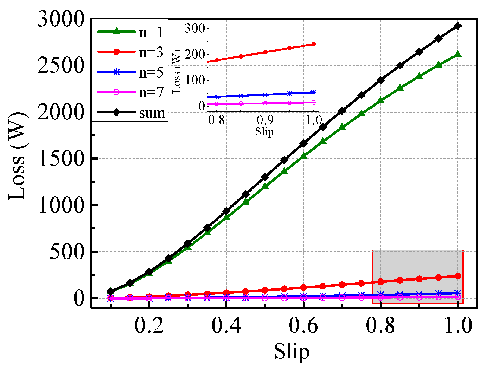
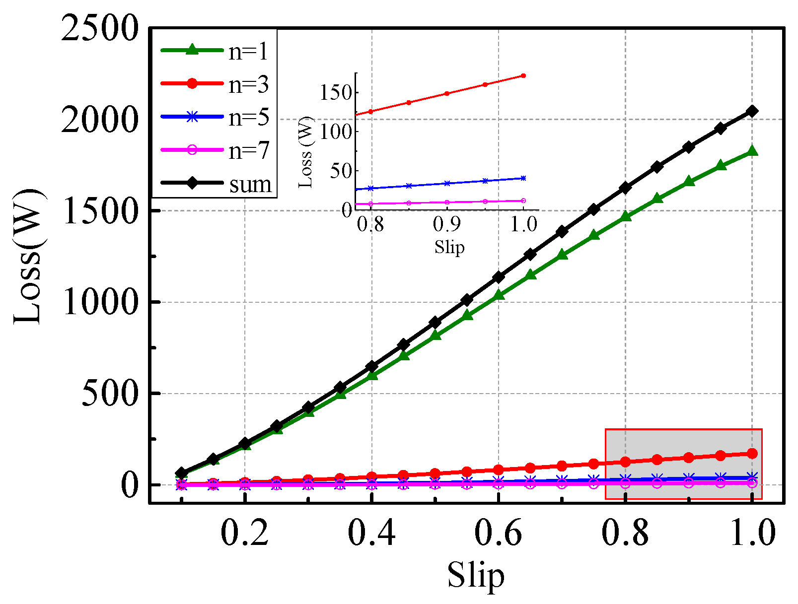
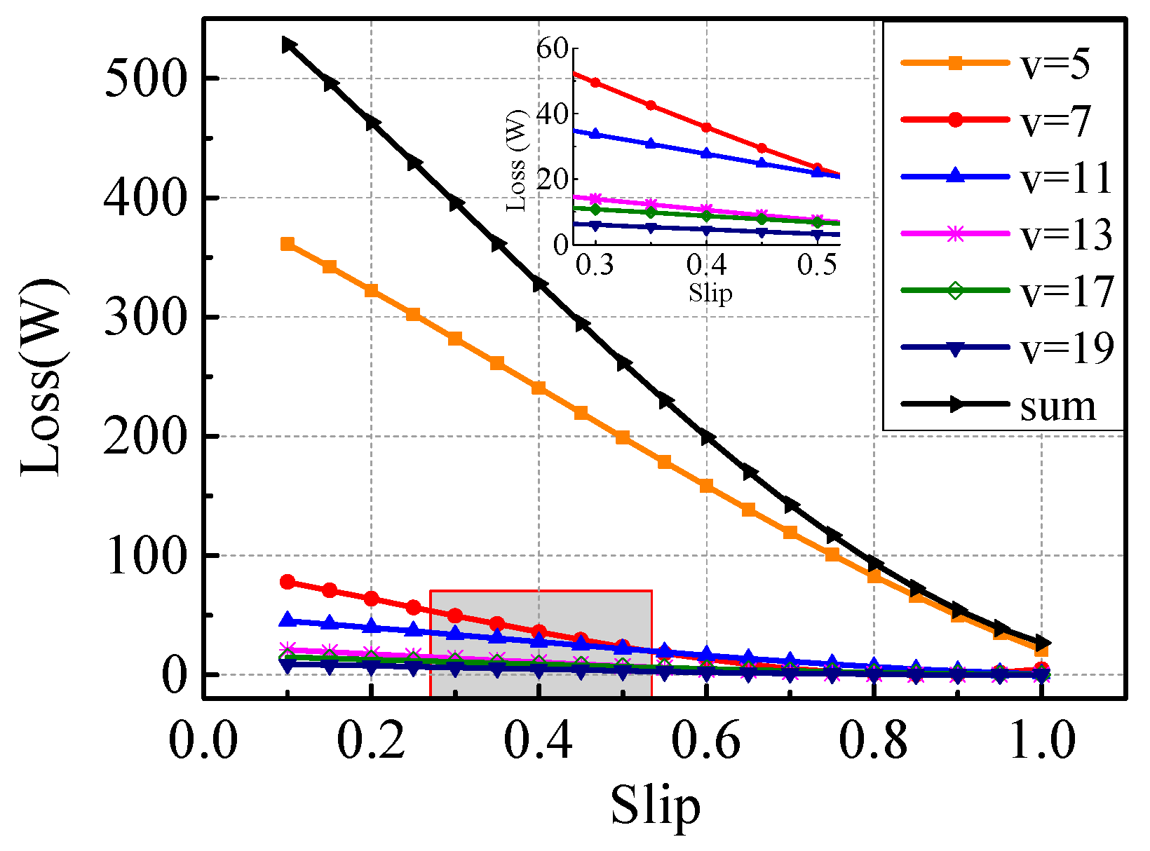
When n = 1, 3, 5, 7, the results of ECLCL and the sum of every component are calculated in different slips, as shown in Figure 3.

Figure 3 shows that all curves increase with the increase of the slip. When the slip is constant, the loss decreases with the increase in n. This phenomenon can be explained by Equations (7), (15), and (16) simultaneously. The vector magnetic potential $\dot{A_{cz}}$ is positively correlated with $\raisebox{1ex}{$1$}\!\left/ \!\raisebox{-1ex}{$n$}\right.$. Thus, $\dot{A_{cz}}$ and the induced current density $j_{cz}$ decrease with increasing n. The fundamental component is the main part of the sum, and the seventh component is close to 0. Thus, the high-order components can be ignored.

3.1.3. Mathematical Model of ECLRC

For the rotor core, the inducted current density is obtained by substitutions in Equations (15) and (16), such as $\dot{A_{cz}}\to \dot{A_{iz}}$, ${\sigma }_{Cu}\to {\sigma }_{Fe}$. The expressions of the inducted current density and ECLRC are as follows [6]:

$$\{\begin{array}{c}\dot{j_{ix}}=0\\ \dot{j_{iy}}=0\\ \dot{\dot{j_{iz}}{=-\sigma }_{Fe}(\frac{\partial \dot{A_{iz}}}{\partial t}{-v}_2\frac{\partial \dot{A_{iz}}}{\partial x})}\\ P_{Fe-eddy}=\frac{1}{2T}{{\displaystyle \int }}_0^T{{\displaystyle \int }}_V\frac{j_{iz}{j}_{iz}^{\ast }}{{\sigma }_{Fe}}dVdt\end{array}$$

(17)

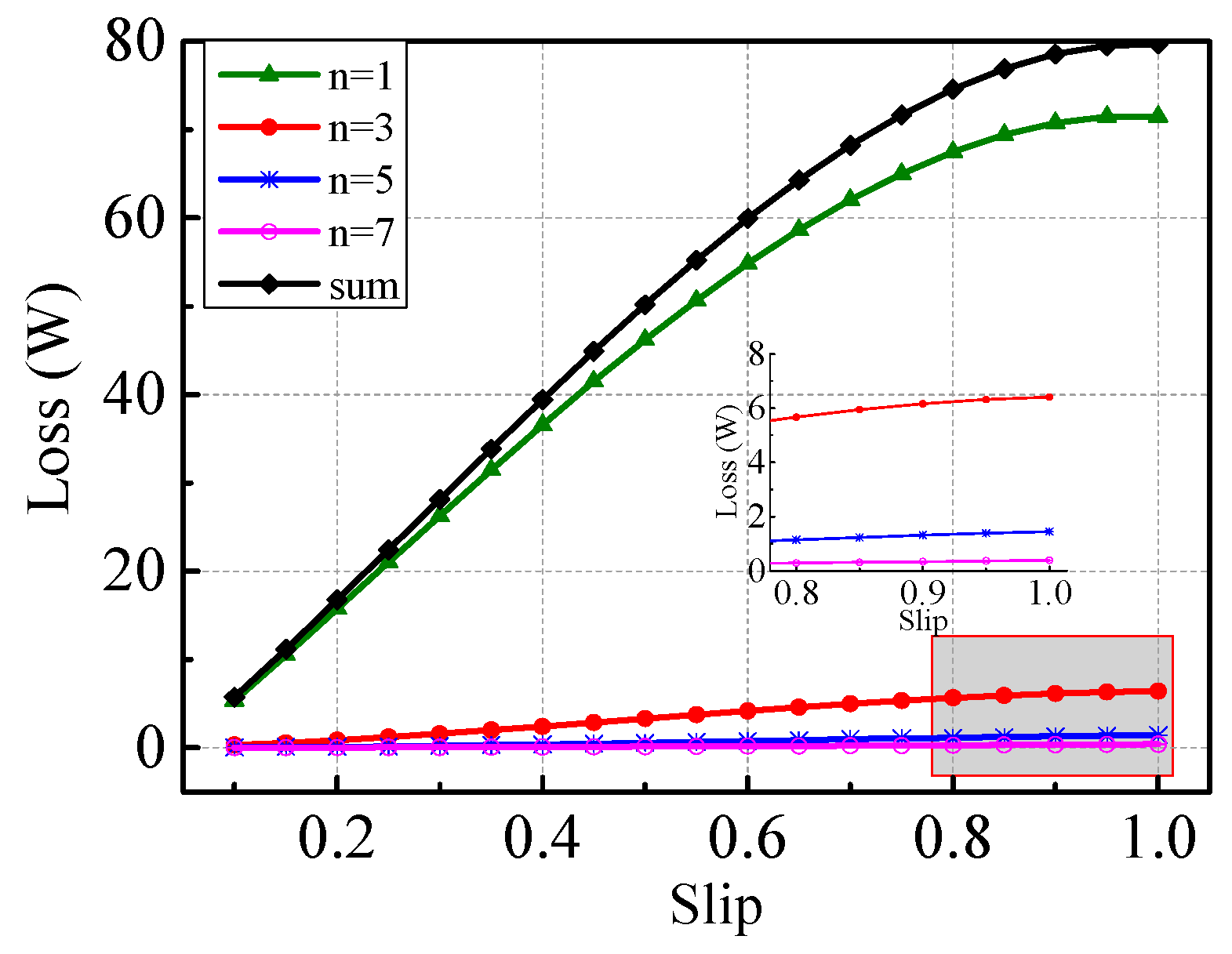
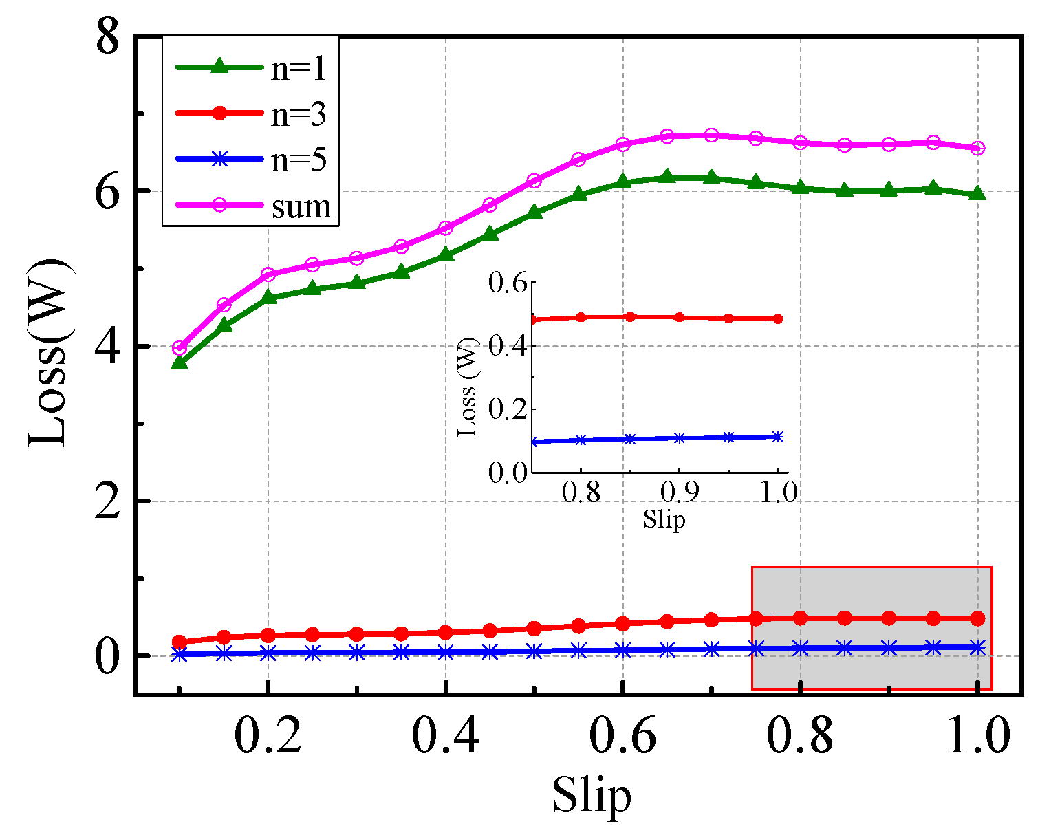
The calculation results of ECLRC and the sum of different slips when n = 1, 3, 5, 7 are shown in Figure 4. Similar to ECLCL, all curves of ECLRC increase with the increase of the slip. When the slip is constant, the loss decreases with the increase in n.

3.2. Nonlinear Analytical Method of ECLCL and ECLRC

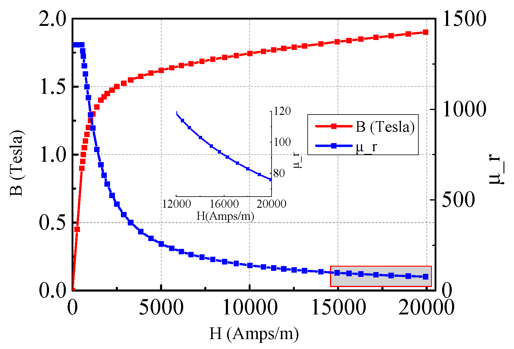
The material of the 2DoFDDIM rotor core is steel, and the saturation effect of the rotor core is ignored, as indicated in Section 3.1. The magnetization (B–H) and relative permeability curves of steel are shown in Figure 5.

Figure 5 shows that the relative permeability is large when the magnetic field strength (H) is small. However, the relative permeability decreases as the magnetic field strength increases, and the relative permeability is small when H is large.

Equation (14) shows that the relative permeability of the rotor core, (${\mu }_r{=\mu }_{Fe}/{\mu }_0$), is an important factor that affects the motor vector magnetic potentials. Thus, when the saturation increases, the influence of a small relative permeability must be considered for an accurate calculation of loss.

According to Equation (2), $\dot{{\mathit{J}}_{sz}}$ is sinusoidal and moves at a synchronous speed along the x-axis. Any point of the stator is selected as a calculating point. Then, the copper layer and rotor core loss powers in the radial direction of this point can be calculated. The computed results multiplied by the corresponding volumes are the ECLCL and ECLRC.

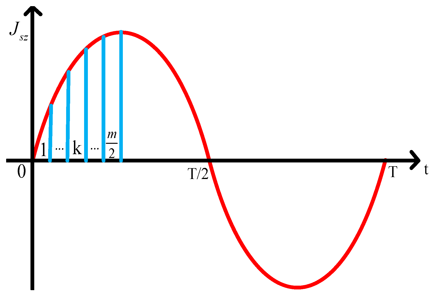
For the calculating point, the saturation differs at different times. In this work, the time period of $\dot{{\mathit{J}}_{sz}}$ is divided into 2m segments (shown in Figure 6) to determine the magnetic field distribution at any time.

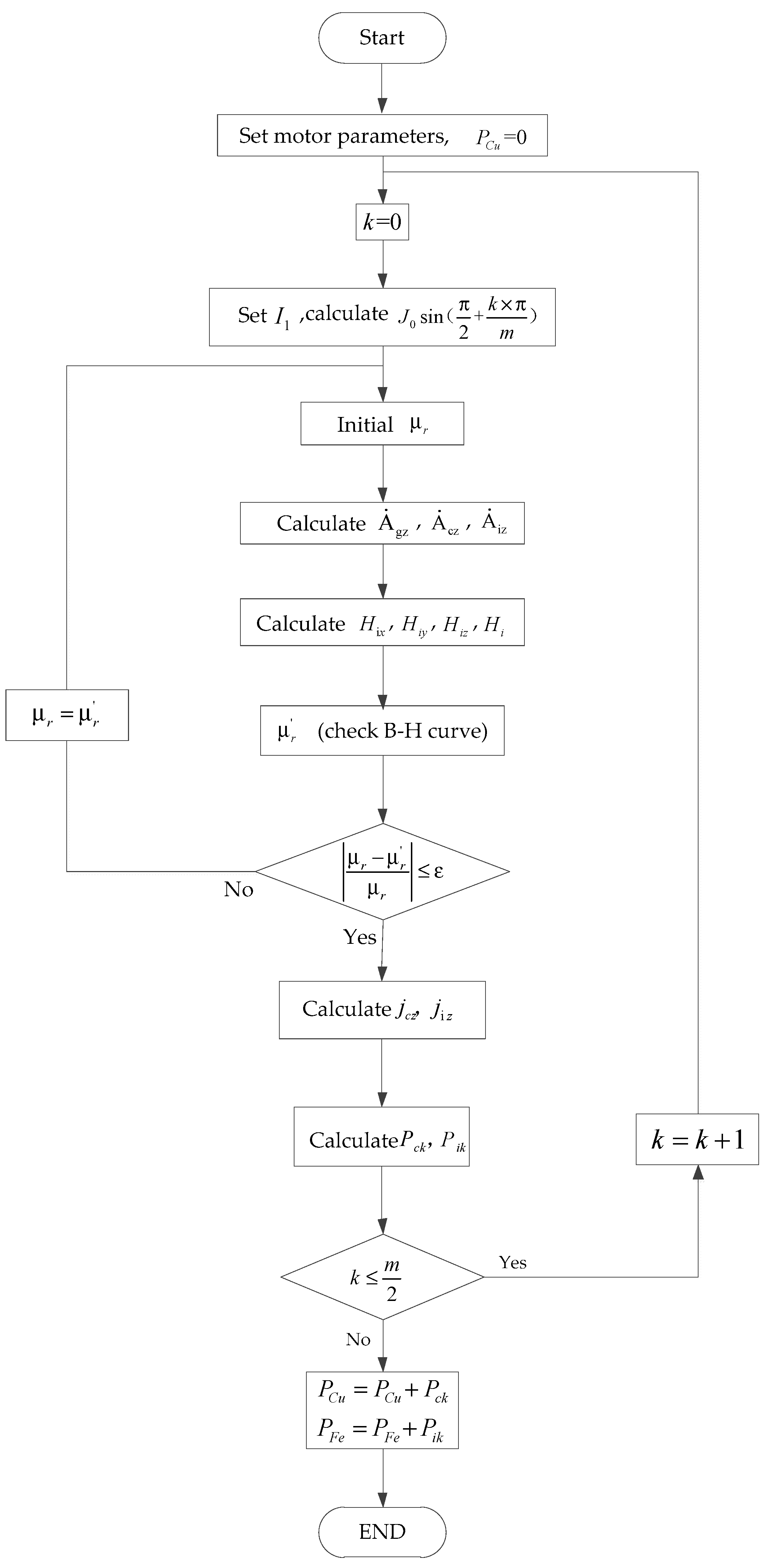
The process of solving magnetic fields while considering saturation is listed below, and Figure 7 shows the computational program diagram of ECLCL.

(1)

Select the calculating point and divide the time period into 2m segments. Owing to the symmetry and parity of $\dot{{\mathit{J}}_{sz}}$, calculating ECLCL and ECLRC in a quarter of the period is sufficient.

(2)

Use ${J=J}_0\sin (\frac{(m-2k)\pi }{2m})$ as an amplitude to establish the expression of $\dot{{\mathit{J}}_{sz}}$, $\dot{{\mathit{J}}_{sz}}={\sum }_n\frac{4}{\pi }{Je}^{{j(\omega }_1{t-ax}_1)}\frac{1}{n}\sin \frac{n\pi }{L_e}z$, $0\le k\le \frac{m}{2}$ (when m is even), $0\le k\le \frac{m-1}{2}$ (when m is odd); k is an integer.

(3)

Assume the initial relative permeability of the calculating point ${\mu }_r$.

(4)

Count the vector magnetic potentials by using ${\mu }_r$.

(5)

On the basis of the relationship between vector magnetic potential and magnetic field strength ($\dot{\mathit{H}}=\frac{1}{\mu }\mathrm{rot}\dot{\mathit{A}}$), obtain the magnetic field strength of the rotor core (H_x, H_y, H_z).

(6)

Compute the magnetic field strength $H=\sqrt{{\left|H_x\right|}^2+{\left|H_y\right|}^2+{\left|H_z\right|}^2}$ and obtain the relative permeability ${\mu }_r^{\prime }$ corresponding to H by checking the B-H curve.

(7)

Calculate the error. If $\left|\frac{{\mu }_r{-\mu }_r^{\prime }}{{\mu }_r}\right|>\epsilon$, ${\mu }_r{=\mu }_r^{\prime }$, return to step 4; otherwise, proceed to the following steps.

(8)

Calculate the inducted current density $\dot{\mathit{J}}$ and the copper layer and rotor core loss powers in one segment by using Equations (15) to (17).

(9)

Multiply the obtained loss powers by the corresponding volumes to obtain ECLCL and ECLRC in one segment.

In this study, m = 11. Hence, $0\le k\le 5$, $s=0.1–1$. The calculated results of the relative permeability obtained by the above-mentioned method are shown in Figure 8. In Figure 8, the x-axis is the slip (s), the y-axis is time (k), and the z-axis is the relative permeability (${\mu }_r$). When n = 1, 3, 5, 7, ECLCL is calculated in different slips, as shown in Figure 9.

Figure 9 shows that the loss of each component increases with the increase of the slip, and the seventh component is close to 0. Thus, the high-order components can be ignored. These are similar to the curves of ECLCL obtained by the linear analysis method shown in Figure 3.

For the rotor core, the vector magnetic potential of the rotor core surface $\dot{{\mathit{A}}_{iz}}$ is obtained by the computational program shown in Figure 7. The distribution of the magnetic field in the rotor core interior is very complicated. Thus, firstly, we ignore the saturation of the rotor core interior and obtain the relative permeability ${\mu }_r$. Then, we calculate the ECLRC. Finally, to consider the influence of eddy, saturation, and end-effects, we correct the results using coefficients.

The material of the rotor core interior is A3 steel. When the saturation of the rotor core interior is neglected, ${\mu }_r=1355.614$ on the basis of the relative permeability curve shown in Figure 5. We substitute the the vector magnetic potential of the rotor core surface $\dot{{\mathit{A}}_{iz}}$ obtained by Figure 7, and ${\mu }_r$ into Equations (7) to calculate the ECLRC. The results are shown in Figure 10.

In Figure 10, all loss curves increase with the increase in slip as long as the slip is small ($s<0.6$), and the curves drop for large slips ($0.6<s<1$). When the slip is larger than 0.6, the stator current increases slightly, such as $I_{s=0.6}=10.5066$, $I_{s=0.8}=11.5066$, $I_{s=1}=11.5808$, and the vector magnetic potential $\dot{{\mathit{A}}_{iz}}$ increases slightly based on Equations (7) and (17). The coefficient ${\alpha }_n$ increases as the slip increases. The influence of ${\alpha }_n$ is large; therefore, $\dot{{\mathit{A}}_{iz}}$ decreases rapidly during the calculation. As a result, the ECLRC decreases. A bulge can be observed at $s=0.2$. The reason is that the time period of sheet current shown in Figure 6 is divided into 22 segments. Ten segments reach saturation when s = 0.2. Fourteen segments reach saturation when s = 0.3. Increasing m can reduce the distortion of the curve.

When the slip increases, the eddy current on the rotor core surface also increases. As a result, the degree of saturation and the tangential current in the end-region increase greatly, the armature reaction caused by the rotor eddy current intensifies, the skin effect is enhanced, and the heat generation caused by power loss increases enormously [21].

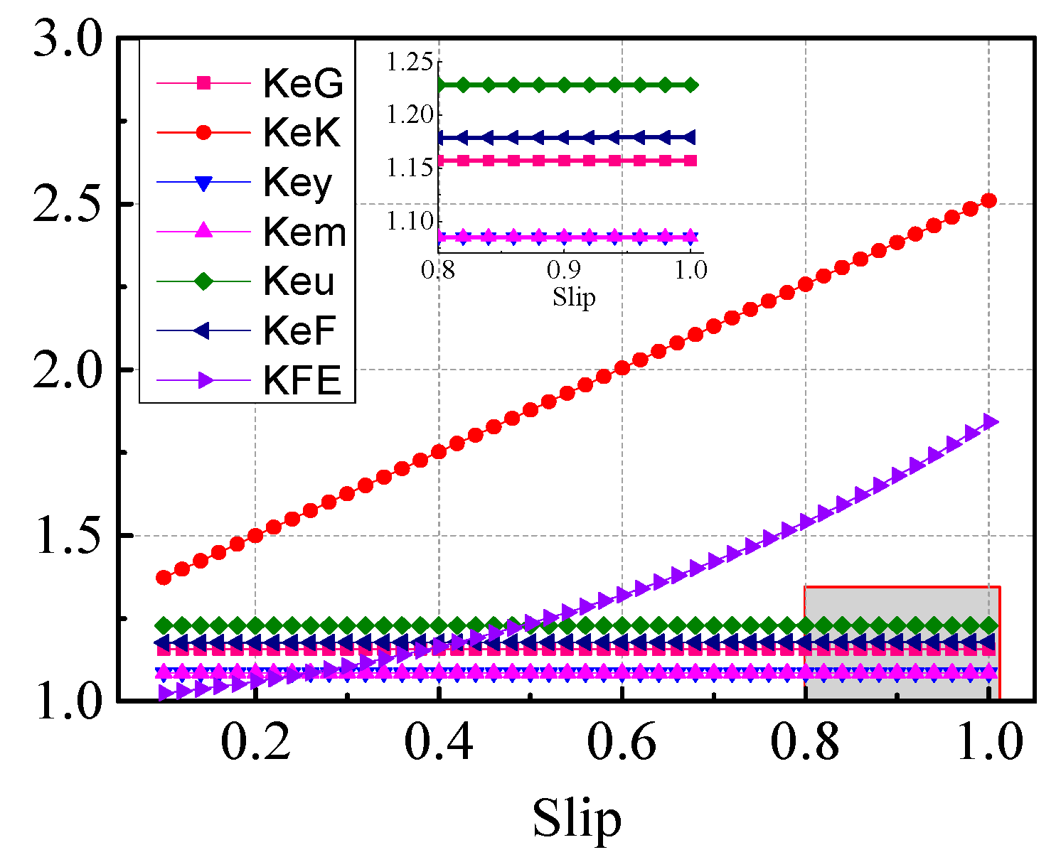
The saturation coefficient $K_{rs}=1.31$ and the eddy coefficient $K_{rc}=0.9$ are used to consider saturation and eddy effects. For the end-region effect, various coefficients were proposed, whose expressions are as follows:

• $K_{eG}$ was proposed by Gibbs [22]:

  $$K_{eG}=1+\frac{2}{\pi }\frac{\tau }{L_e}$$

  (18)
• $K_{eK}$ was proposed by Kesavamurthy [23]:

  $$K_{eK}=(1+\frac{\tau }{L_e}\left)\right(1+\frac{s}{4}\frac{L_e}{\tau })$$

  (19)
• $K_{ey}$ was proposed by Yee [24]:

  $$K_{ey}=1+\frac{\frac{2}{\pi }\frac{\tau }{L_e}}{1+\coth \left(\frac{\pi }{2}\frac{L_e}{\tau }\right)-\frac{2}{\pi }\frac{\tau }{L_e}}$$

  (20)
• $K_{em}$ was proposed by Mokirinihoph [25]:

  $$K_{em}=\frac{1}{1-\frac{2\tau }{{\pi L}_e}\frac{\mathrm{ch}(\frac{\pi }{2}\frac{L_e}{\tau }\left)\mathrm{sh}\right(\frac{\pi }{2}\frac{L_e}{\tau })}{\mathrm{ch}(\frac{\pi }{2}\frac{L_e{+D}_2}{\tau })}}$$

  (21)
• $K_{eu}$ was proposed by Lee Tesor [26]:

  $$K_{eu}=1+\frac{D_2}{L_e}\sin \frac{\pi }{2p}$$

  (22)
• $K_{eF}$ was proposed by Fengli Fu and Jinming Lin [27]:

  $$K_{eK}=(1+\frac{\tau }{L_e}\left)\right(\frac{a^2\delta +\frac{1}{{\mu }_r∆}}{{\lambda }_1^2+\frac{1}{{\mu }_r∆}})$$

  (23)

  where $a=\frac{\pi }{\tau }$, ${\lambda }_1=a\sqrt{1+{\left(\frac{\tau }{L_e}\right)}^2}$, and $∆$ is the penetration depth.

Figure 11 shows that none of the aforementioned coefficients can express the relationship between slip and the end-region effect accurately. Thus, Yan Hu proposed a new end-region coefficient, $K_{FE}$. It can be written in terms of slip as follows [28]:

$$K_{FE}={(\frac{K_{eK}{+K}_{eF}}{2})}^s$$

(24)

The curves of all coefficients are shown in Figure 11.

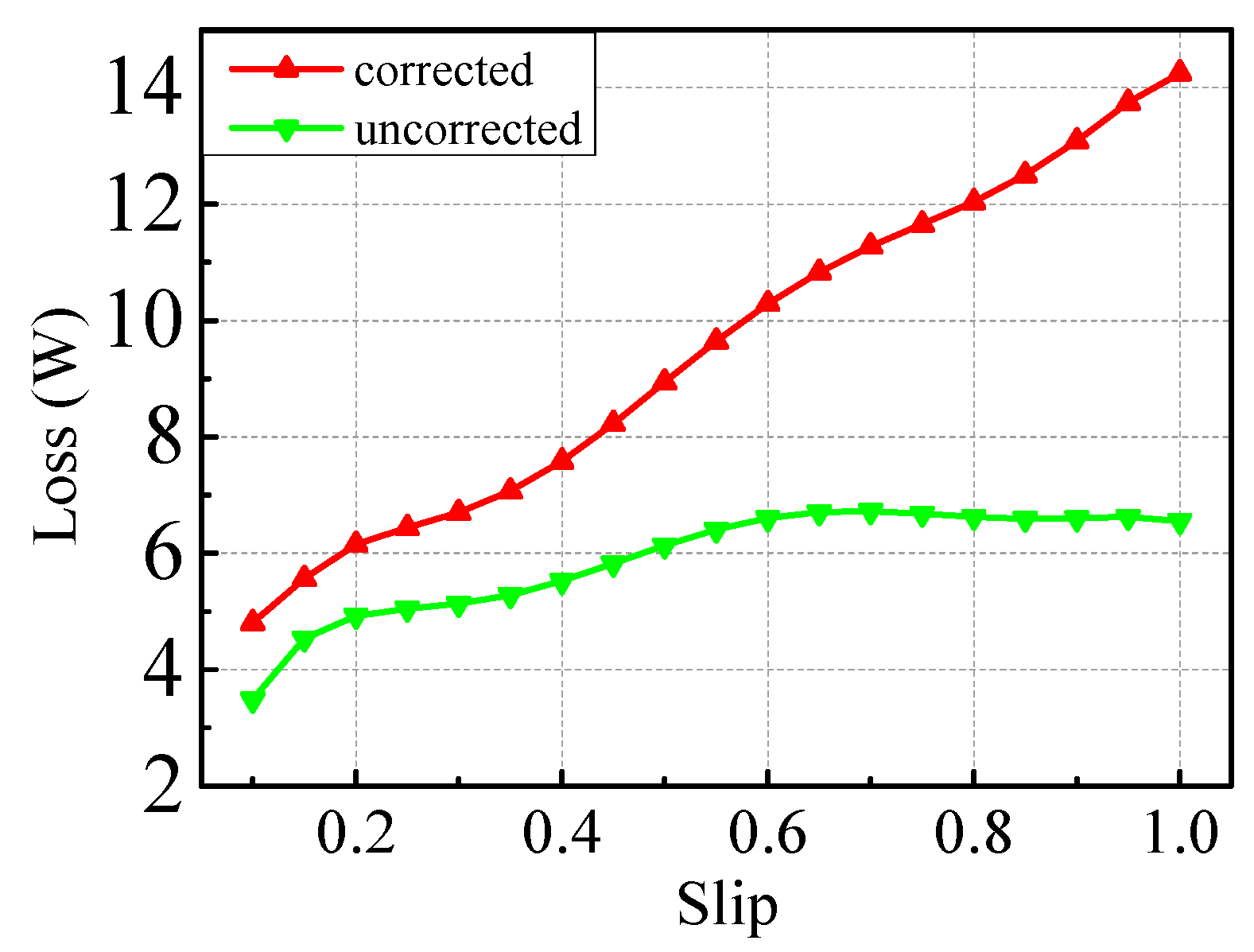
$K_{FE}$ is selected in this study and the uncorrected and corrected nonlinear analysis results of ECLRC are shown in Figure 12.

Figure 12 shows that the uncorrected nonlinear analysis results of ECLRC are increased by the coefficients. The curve of the corrected nonlinear analysis results of ECLRC increases with the increase of the slip.

3.3. Analytical Model of SECLCL and SECLRC

The air gap of the solid-rotor induction motor has fundamental and high-order harmonic magnetic fields. The eddy losses caused by the harmonic fields, which are distributed on the rotor surface, are called surface eddy current losses [29]. For the studied motor, the following assumptions are proposed to simplify the analysis and calculation.

(1)

The materials of the rotor and stator are isotropic. The primary cores have infinite permeability and resistance.

(2)

The curvature effect is neglected. The currents only include the z-component.

(3)

The time variation of each harmonic field is sinusoidal.

The 2D analysis model is shown in Figure 13. The rectangular coordinate system is fixed on the rotor.

The harmonic fields are sinusoidal on the basis of the assumptions. The traveling magnetic field is $B_{vy(y=0)}=\sqrt{2}{B}_{xy0}{\sin (\omega }_{v}t-\frac{\pi }{{\tau }_v}x)$. The 2D eddy equation and Maxwell second equation are as follows:

$${\nabla }^2\dot{{\mathit{H}}_{vy}}{=j\omega }_v\mu \sigma \dot{{\mathit{H}}_{vy}}$$

(25)

$$\nabla {\times E}_v=-\frac{\partial B_v}{\partial t}$$

(26)

Expression (25) can be solved by separation of the variables, and the expression of the magnetic field strength on the rotor surface is established on the basis of the relationship between magnetic field strength and magnetic density, $B=\mu H$, as follows:

$$H_{vy}=\sqrt{2}{H}_{vy0}{e}^{-ay}\sin \left({\omega }_{v}t-\frac{\pi }{{\tau }_v}x-by\right)$$

(27)

where v expresses the harmonic order, and ${\omega }_v$, ${\tau }_v$, $B_{vy0}$, and $H_{vy0}$ indicate the angular frequency relative to the rotor, the polar distance, the effective value of the rotor surface magnetic density, and the magnetic field strength, respectively; $a=\left|\gamma \right|\cos \phi$, $b=\left|\gamma \right|\sin \phi$, and ${\gamma }^2={\left(\frac{\pi }{{\tau }_v}\right)}^2+j\omega \mu \sigma$. The rotor current is assumed to include the axial component. Hence, $\dot{\mathit{E}}=\overrightarrow{k}{E}_z$. The expression of the electric field strength is obtained by solving Equations (26) and (27):

$$E_{zv}=\frac{{\omega }_v\sqrt{2}{B}_{vy0}}{\pi /{\tau }_v}{e}^{-ay}\sin \left({\omega }_{v}t-\frac{\pi }{{\tau }_v}x-by\right)$$

(28)

The eddy current loss is calculated by the following equation.

$$P_v={{\displaystyle \int }}_v\frac{1}{2}{\sigma |E}_{vm}{|}^2\mathrm{dv}$$

(29)

where E_vm denotes the amplitude of the electric field intensity generated by the v-th order harmonic. When the edge effect is ignored, the Equation (22) is simplified as [10]:

$$P_v=\frac{D\pi \sigma L_e}{2}{{\displaystyle \int }}_{d_{in}}^{d_{out}}{\left(\frac{{\omega }_v{B}_{vy0}}{\pi /{\tau }_v}{e}^{-ay}\right)}^{2}dy$$

(30)

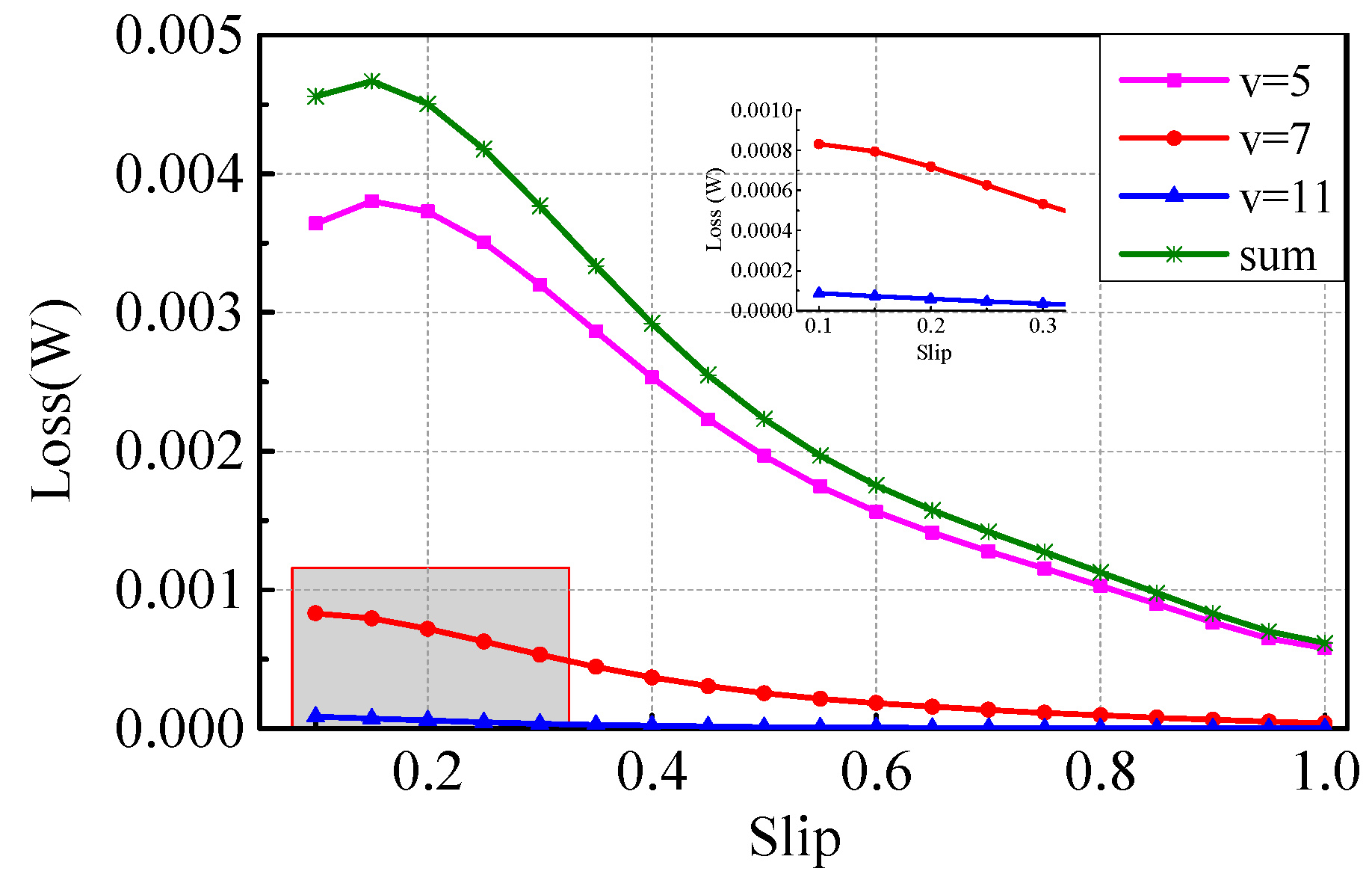
where $D$ expresses each layer’s outer diameter. SECLCL and SECLRC are calculated by substituting the corresponding parameters into Equation (23), and the results are shown in Figure 14 and Figure 15.

Overall, all curves tend to decrease with the increase of the slip. The results of SECLRC are extremely small. The eleventh component is close to zero. Thus, the high-order components can be ignored.

4. Results Comparison and Analysis

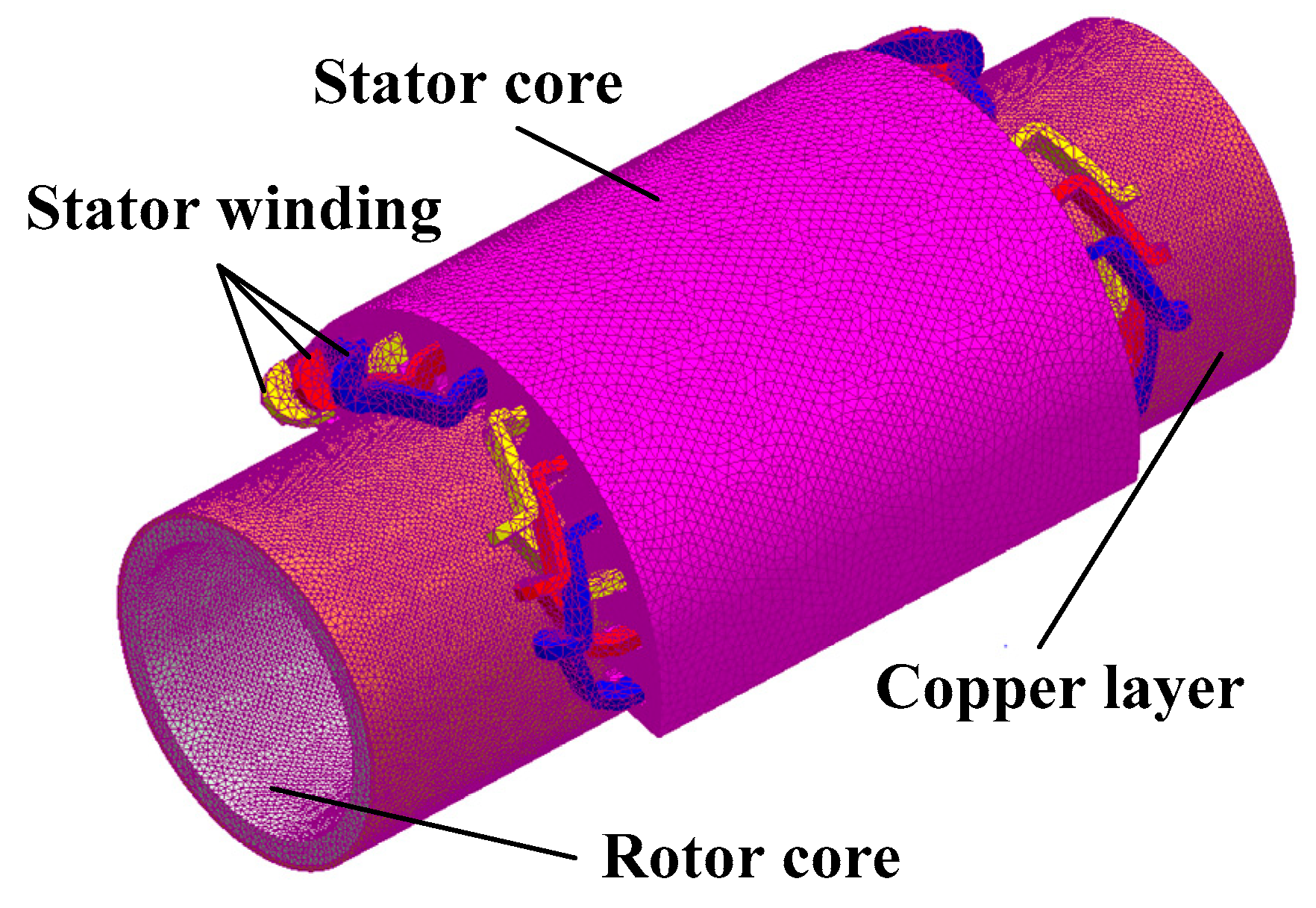
To verity the new analysis method, a 3D finite element model is established based on the parameters listed in Table 1, as shown in Figure 16. TECLs in the copper layer and rotor core can be calculated by Equation (1).

4.1. Copper Layer TECL

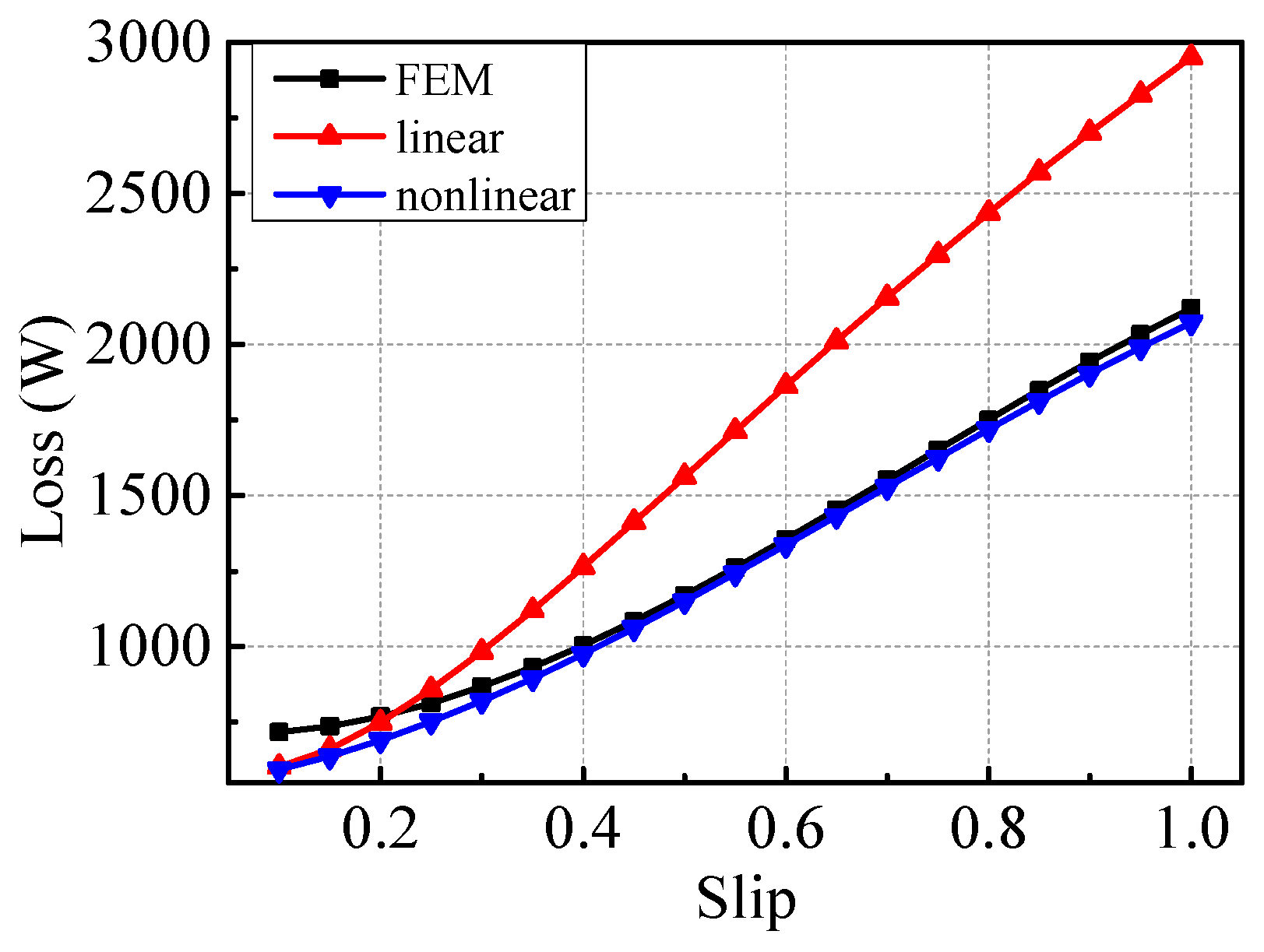
TECLs in the copper layer obtained by FEM, the original linear analytical method, and the new nonlinear analytical method, are compared. The results are shown in Figure 17 and

Table 2. TECL in the copper layer.

Slip	FEM (W)	Linear (W)	Error (%)	Nonlinear (W)	Error (%)
0.1	717.33	602.037	16.07	592.333	17.43
0.2	769.09	748.601	2.664	690.507	10.22
0.3	867.74	983.466	13.34	820.599	5.433
0.4	1004.3	1264.13	25.87	976.030	2.818
0.5	1169.9	1563.02	33.60	1150.22	1.684
0.6	1355.6	1863.41	37.46	1336.60	1.399
0.7	1552.3	2155.96	38.89	1528.57	1.529
0.8	1751.2	2435.95	39.10	1719.57	1.806
0.9	1943.3	2701.24	39.04	1903.02	2.074
1	2119.7	2950.84	39.21	2072.34	2.235

.

Figure 17 and Table 2 show that the three curves have the same trend. When the saturation effect is ignored, the analysis values are greater than the simulation values in large slips ($s\ge 0.3$), and the error increases as the slip increases. When the new analysis method that considers the nonlinearity of the rotor core surface is adopted, the analysis values are reduced obviously, and the calculation accuracy is improved. Most errors are less than 15%, except for the error when $s=0.1$, which is 17.43%. The errors are acceptable. Hence, the new analysis method is valid. Partial errors are greater than 5% ($0.3\ge s\ge 0.1$). The reasons for these phenomena are as follows:

(1)

With the increase in slip, the saturation of the rotor core increases. When the saturation is ignored, the relative permeability of the rotor core is much higher than the actual value, and the magnetic density and analysis value of the loss are large. The new method, which considers the nonlinearity of the rotor core, can improve the accuracy of the rotor core’s relative permeability. Thus, the rotor core’s relative permeability decreases, and the loss analysis value decreases.

(2)

The radial inducted current is disregarded. The FEM can consider the loss caused by the radial inducted current.

(3)

Owing to the stator circumferential breaking structure, the longitudinal edge effect is formed at the stator end. The end magnetic field and the end induced current caused by the longitudinal edge effect increase the loss in the rotor. According to Assumptions 2 in Section 3.1, the edge effect is ignored in the analysis calculation, so the error increases.

(4)

In this work, the period of surface current density $\dot{{\mathit{J}}_{sz}}$ is divided into 22 segments (m = 11); m is not large enough and influences the accuracy.

4.2. Rotor Core TECL

TECLs in the rotor core obtained by the three methods are shown in Figure 18 and

Table 3. TECL in the rotor core.

Slip	FEM (W)	Linear (W)	Error (%)	Nonlinear (W)	Error (%)
0.1	4.837	5.719	18.24	4.808	0.593
0.2	6.028	16.75	177.8	6.158	2.167
0.3	7.100	28.14	296.3	6.702	5.596
0.4	8.078	39.44	388.3	7.587	6.068
0.5	8.985	50.19	458.7	8.942	0.474
0.6	9.844	59.94	508.9	10.29	4.546
0.7	10.68	68.22	538.7	11.28	5.591
0.8	11.52	74.59	547.6	12.04	4.551
0.9	12.38	78.57	534.7	13.09	5.738
1	13.29	79.72	499.8	14.25	7.233

.

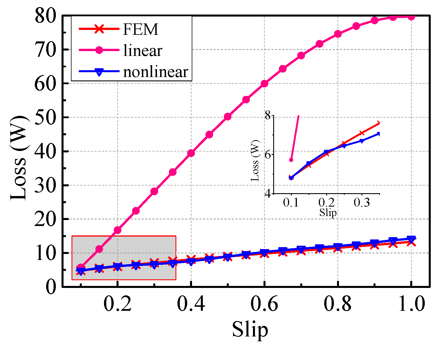
The difference of the errors between the results obtained by the linear analytical method and FEM is remarkable. The new nonlinear analytical method can obviously improve the accuracy, and the errors are $177.8\%–547.6\%$ down to less than 7.3%. The errors are acceptable. The values of the analysis results are mostly smaller than the simulation ones, and the reason is that the losses caused by the radial and tangential induced currents are ignored.

5. Conclusions

In this paper, a 2DoFDDIM whose solid rotor is coated with a copper layer, is regarded as the research object. TECLs in the copper layer and rotor core of the rotary part are calculated using analytical methods. Comparison of the values obtained by the linear analytical method, nonlinear analytical method, and 3D FEM yields the following conclusions:

(1)

For TECL in the copper layer, most errors are less than 6%, except for $s$ = 0.1–0.2. For the rotor core, the errors of the corrected nonlinear analysis results are less than $7.3\%$. Hence, the new analytical method is valid.

(2)

In this paper, the time period of $\dot{{\mathit{J}}_{sz}}$ is divided into 2m = 22 segments. The value of m influences calculation accuracy. Calculation accuracy and computation time increase with the increase of m.

(3)

Induced current is observed in the radial direction, and the edge effect occurs at the stator end. Hence, the calculation values are lower than those determined in the simulation, as shown in Figure 17 and Figure 18. The new nonlinear analytical method requires modifications to consider the edge effect and radial induced current.

References

- Si, J.K.; Ai, L.W.; Xie, L.J. Analysis on Electro-magnetic Field and Performance Calculation of 2-DoF Direct Drive Induction Motor. Trans. China Electrotech. Soc. 2015, 30, 153–160. [Google Scholar]
- Si, J.K.; Xie, L.J.; Cao, W.P. Performance analysis of the 2DoF direct drive induction motor applying composite multilayer method. IET Electr. Power Appl. 2017, 11, 524–531. [Google Scholar] [CrossRef]
- Si, J.K.; Si, M.; Xu, X.Z. Effects of rotor conduction material and air gap length on performance of linear are-shaped induction motor. Electr. Mach. Control 2012, 16, 31–37. [Google Scholar]
- Si, J.K.; Feng, H.C.; Ai, L.W. Design and Analysis of a 2-DOF Split-Stator Induction Motor. IEEE Trans. Energy Convers. 2015, 30, 1200–1208. [Google Scholar] [CrossRef]
- Lv, G.; Zeng, D.H.; Zhou, T. Analysis of Secondary Losses and Efficiency in Linear Induction Motors with Composite Secondary Based on Space Harmonic Method. IEEE Trans. Energy Convers. 2017, 32, 1583–1591. [Google Scholar] [CrossRef]
- Lv, G.; Zeng, D.; Zhou, T. Investigation of Forces and Secondary Losses in Linear Induction Motor with the Solid and Laminated Back Iron Secondary for Metro. IEEE Trans. Energy Convers. 2017, 64, 4382–4390. [Google Scholar] [CrossRef]
- Kou, B.Q.; Jin, Y.X.; He, Z. Nonlinear Analytical Modeling of Hybrid-Excitation Double-Sided Linear Eddy-Current Brake. IEEE Trans. Magn. 2015, 51, 1–4. [Google Scholar] [CrossRef]
- Shah, M.R.; Lee, S.B. Optimization of Shield Thickness of Finite-Length Solid Rotors for Eddy-Current Loss Minimization. IEEE Trans. Ind. Appl. 2009, 45, 1947–1953. [Google Scholar] [CrossRef]
- Shah, M.R.; Lee, S.B. Rapid Analytical Optimization of Eddy Current Shield Thickness for Associated Loss Minimization in Electrical Machines. IEEE Trans. Ind. Appl. 2006, 42, 642–649. [Google Scholar] [CrossRef]
- Chang, Z.F.; Huang, W.X.; Hu, Y.W. Research on Stray Loss of Smooth Surface Solid Rotor Induction Motor Based on 2D Analytical Approach. Proc. CSEE 2007, 27, 83–88. [Google Scholar]
- Si, J.K.; Xie, L.J.; Feng, H.C. Mathematical Model of Two-Degree-of-Freedom Direct Drive Induction Motor Considering Coupling Effect. J. Electr. Eng. Technol. 2017, 12, 1227–1234. [Google Scholar] [CrossRef]
- Si, J.K.; Xie, L.J.; Xu, X.Z. Static coupling effect of a two-degree-of-freedom direct drive induction motor. IET Electr. Power Appl. 2017, 11, 532–539. [Google Scholar] [CrossRef]
- Zhang, M.Y.; Xia, D.W.; Wang, D.Q. Distribution on the magnetic field of a composite-rotor induction motor. J. Qingdao Univ. 1995, 10, 1–9. [Google Scholar]
- Si, J.K.; Ai, L.W.; Han, J.B. Characteristic analysis of no-load speed of linear induction motor. Electr. Mach. Control 2014, 18, 37–43. [Google Scholar]
- Zhang, M.Y.; Pan, M.Y.; Xia, D.W. Electromagnetic field analysis and end factor determination for a composite rotor motor. Proc. CSEE 1995, 15, 239–246. [Google Scholar]
- Xiao, R.H.; Zhang, M.Y. The analyses and calculation on induction motor with copper-surfaced solid rotors by multi-layer theory. J. Shandong Univ. 1991, 21, 42–49. [Google Scholar]
- Lv, G.; Liu, Z.M.; Sun, S.G. Electromagnetism calculation of single-sided linear induction motor with transverse asymmetry using finite-element method. IET Electr. Power Appl. 2016, 10, 63–73. [Google Scholar] [CrossRef]
- Cheaytani, J.; Benabou, A.; Tounzi, A. Stray Load Losses Analysis of Cage Induction Motor Using 3-D Finite-Element Method with External Circuit Coupling. IEEE Trans. Magn. 2017, 53, 1–4. [Google Scholar] [CrossRef]
- Yamada, T.; Fujisaki, K. Basic Characteristic of Electromagnetic Force in Induction Heating Application of Linear Induction Motor. IEEE Trans. Magn. 2008, 44, 4070–4073. [Google Scholar] [CrossRef]
- Aho, T.; Nerg, J.; Pyrhonen, J. Analyzing the effect of the rotor coating on the rotor losses of medium-speed solid-rotor induction motor. In Proceedings of the International Symposium on Power Electronics, Electrical Drives, Automation and Motion (SPEEDAM 2006), Taormina, Italy, 23–26 May 2006. [Google Scholar]
- Bi, D.Q.; Wang, X.H.; Li, D.C. Magnetic analysis and design method for solid rotor induction motors based on directly coupled field-circuit. In Proceedings of the Third International Power Electronics and Motion Control Conference (IPEMC 2000), Beijing, China, 15–18 August 2000. [Google Scholar]
- Gibbs, W. Induction and synchronous motors with unlaminated rotors. J. Inst. Electr. Eng. 1948, 95, 411–420. [Google Scholar]
- Kesavamurthy, N.; Rajagopolan, P.K. The Polyphase Induction Machine with Solid Iron Rotor. Trans. Am. Inst. Electr. Eng. 1959, 78, 1092–1098. [Google Scholar] [CrossRef]
- Yee, H. Effects of finite length in solid-rotor induction machines. Proc. Inst. Electr. Eng. 1971, 118, 1025–1033. [Google Scholar] [CrossRef]
- Tang, X.G.; Ning, Y.Q.; Fu, F.L. Solid Rotor Asynchronous Motor and Its Application, 1st ed.; China Machine Press: Beijing, China, 1991. (In Chinese) [Google Scholar]
- Fu, F.L.; Tang, X.G. Handbook of Induction Motor Design, 2nd ed.; China Machine Press: Beijing, China, 2006. (In Chinese) [Google Scholar]
- Fu, F.L.; Lin, J.M. End coefficient calculation of solid rotor asynchronous motor. S&M Electr. Mach. 1986, 3, 5–9. [Google Scholar]
- Hu, Y.; Chen, J.Z.; Ding, X.Y. Analysis and Computation on Magnetic Field of Solid Rotor Induction Motor. IEEE Trans. Appl. Supercon. 2010, 20, 1844–1847. [Google Scholar]
- Chang, Z.F. Composite Rotor Induction Motor Electromagnetic Calculation. Master’s Thesis, Nanjing University of Aeronautics and Astronautics, Nanjing, China, 2007. [Google Scholar]
Figure 1.
Structure of the two-degree-of-freedom direct-drive induction motor (2DoFDDIM). (a) Rotary motion arc-shape stator; (b) Linear motion arc-shape stator; (c) Rotor; (d) Assembly of 2DoFDDIM.
Figure 2.
Expanded plate model of the rotary part.
Figure 3.
Eddy current loss in the copper layer (ECLCL) neglecting the saturation effect.
Figure 4.
Eddy current loss in the rotor core (ECLRC) neglecting the saturation effect.
Figure 5.
B–H and relative permeability curves of steel.
Figure 6.
Curve of the divided surface current density.
Figure 7.
Computational program diagram of ECLCL and ECLRC.
Figure 8.
Relative permeability of the rotor core.
Figure 9.
ECLCL considering the nonlinearity of the rotor core.
Figure 10.
ECLRC considering the nonlinearity of the rotor core.
Figure 11.
End-region coefficients versus slip.
Figure 12.
Uncorrected and corrected nonlinear analysis results.
Figure 13.
2D analysis model of the motor.
Figure 14.
Analysis results of surface eddy current losses in the copper layer (SECLCL).
Figure 15.
Analysis results of surface eddy current losses in the rotor core (SECLRC).
Figure 16.
3D finite element method (FEM) of the rotary part.
Figure 17.
Total eddy current loss (TECL) in the copper layer.
Figure 18.
TECL in the rotor core.