A New Adaptive Approach to Control Circulating and Output Current of Modular Multilevel Converter
by
 , ,
, ,
Muhammad Ishfaq
1,* ,
,
Waqar Uddin
1,*, 
Kamran Zeb
1,2 ,
,
Imran Khan
1, 
Saif Ul Islam
1,
Muhammad Adil Khan
3 and
Hee Je Kim
1,* 1
Department of Electrical Engineering, Pusan National University Busan, South Korea San 30, ChangJeon Dong, Pusandaehak-ro 63 7 beon-gil 2, Geumjeong-gu, Busan-city-46241, Korea
2
Department of Electrical and Computer Science, National University of Engineering and Technology, Islamabad City 44000, Pakistan
3
Department of Electrical and Computer Science, Air University, Islamabad City 44000, Pakistan
*
Authors to whom correspondence should be addressed.
Energies 2019, 12(6), 1118; https://doi.org/10.3390/en12061118
Submission received: 1 February 2019
/
Revised: 15 March 2019
/
Accepted: 19 March 2019
/
Published: 22 March 2019
(This article belongs to the Special Issue Design and Control of Power Converters 2019)
Abstract
:This paper addresses the output current and circulating current control of the modular multi-level converter (MMC). The challenging task of MMCs is the control of output current and circulating current. Existing control structures for output and circulating current achieve control objectives with comparatively complex controllers and the designed parameters for the controller is also difficult. In this paper, an adaptive proportional integral (API) controller is designed to control the output current and the circulating current. The output current is regulated in axes while the circulating current is regulated in the stationary frame to enhance MMC performance. The output and circulating current control results using an API controller are compared with the conventional proportional resonant (PR) controller in terms of transient response, stability, optimal performance, and reference tracking for results verification. The API control architecture significantly improve transient response, stability, and have excellent reference tracking capability. Moreover, it controls output current and converges the circulating current to a desired value. The control structure is designed for a three-phase MMC system, simulated and analyzed in MATLAB-Simulink.
1. Introduction
The MMC is becoming an increasingly attractive, competitive, and highly applied technology for medium and high voltage power applications due to its advantages, such as low harmonics, modular structure, simple scaling, loss reduction in switches, and satisfactory fault management [1,2,3]. Currently, MMCs have been expanded to many applications [4] such as motor drivers [5], solar/wind power systems [6,7,8], energy transmission and distribution systems [9], and static synchronous compensators (STATCOM) [10]. Recently published literature related to MMC targeted current control, voltage control, loss analysis and modulation, dynamic and steady-state models, modeling, and simulation methods [11,12,13,14,15,16].
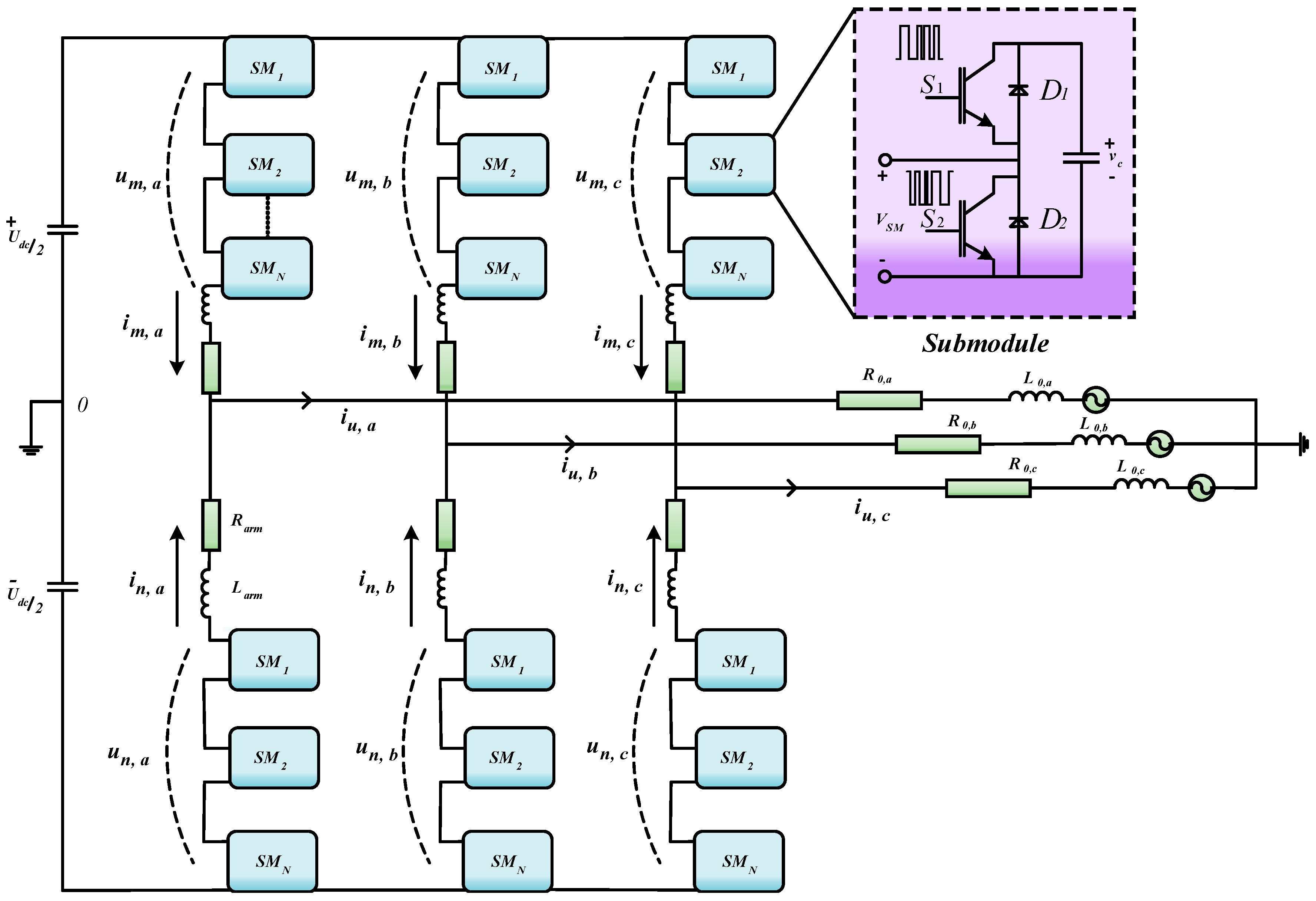
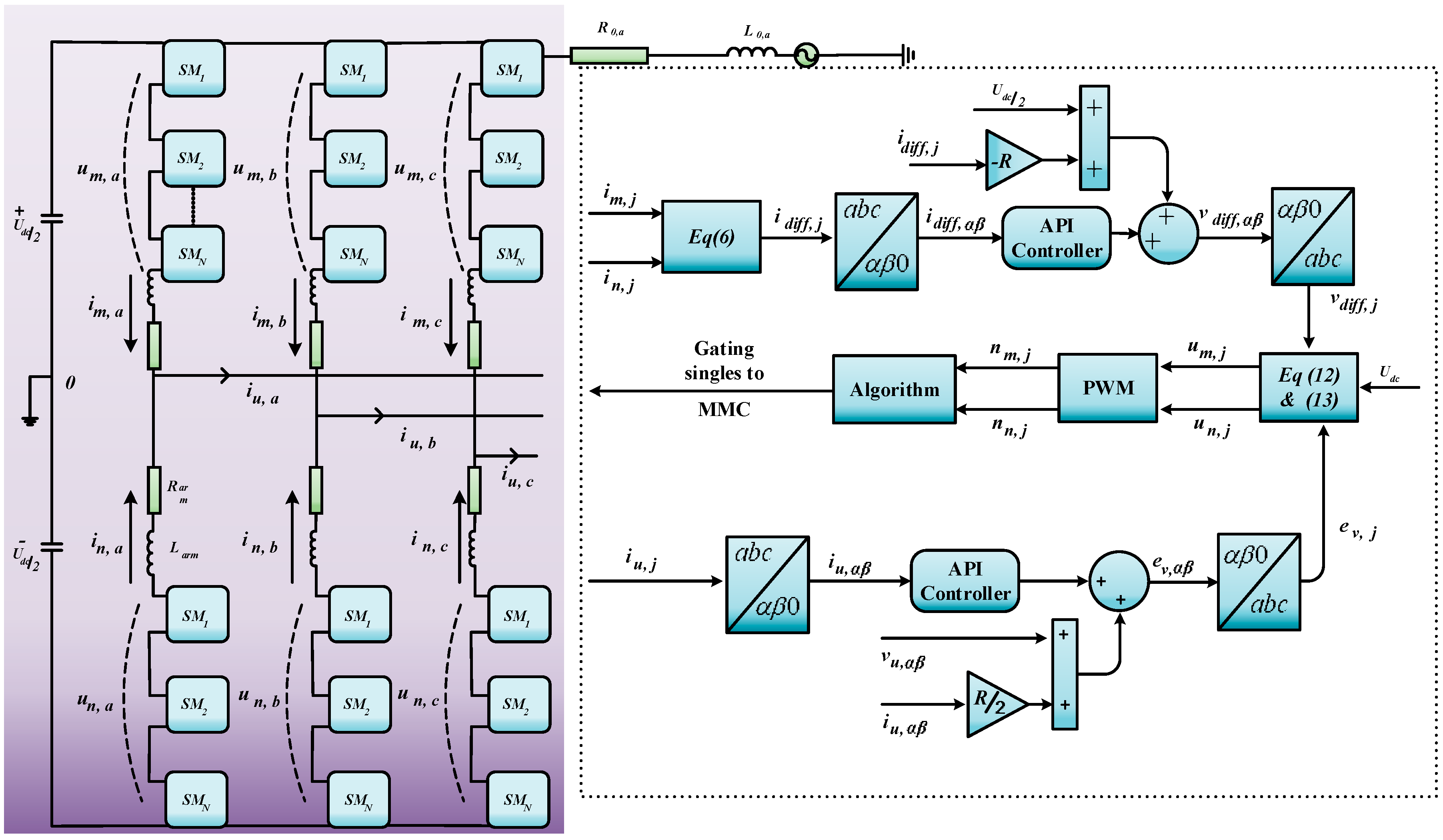
The first structure of the MMC was presented in [17]. Currently, many configurations and control designed approaches have been introduced by many researchers for the control objectives, such as balancing and averaging of SM capacitor voltage, circulating current ripples injection or suppression, and output voltage regulation [18,19,20,21,22]. Figure 1 shows the configuration of a three-phase six arm MMC. Every arm of the MMC is equipped with a series connected sub module (SM) configuration. The SM, consists of two switches connected with a capacitor, is also depicted in Figure 1.
For the optimal performance of MMC, the control system plays a vital role. The output current is controlled to transfer the power to AC grid while the circulating current does not affect the output of the converter. However, uncontrolled circulating current results in higher losses. The circulating current problem in each arm of MMC arises due to potential differences in every SM arm and DC link. Reference [23] studied the effects of arm inductance and SM capacitance on the magnitude of circulating current. Increases in arm inductance decrease the circulating current, but the circulating currents are not eliminated. The negative sequence component of circulating current rotates at twice line frequency. A control scheme is proposed in [24] by translating the a-b-c sequence components into rotational frame. But this control structure has a limitation because the circulating current also have positive and zero sequence components along with negative sequence components.
The most common control approach was introduced by Hagiwara and Akagi in [25]. The control method is used to regulate the output current and internal dynamics, i.e., circulating current and internal energy. However, the ripples in circulating current could not be eliminated effectively by this control method. Over the past few years, many control schemes for circulating current were proposed such as or rotating frame control for the suppression of 2nd order harmonics [26,27,28], resonant controllers to eliminate harmonics in unbalanced circumstances [29] and to eliminate integral harmonics in circulating currents plug in repetitive controllers are used [30,31]. But the above-mentioned control method is complicated in structure and the controllers are difficult to tune for system stability and performance.
Some researchers have proposed control methods for controlling both circulating current and output current. A PR control strategy is used to control an output current to get the desired output power. The output current is 1st harmonic frequency sinusoid [32]. Since after all PR control strategy gives an infinite gain at the resonant frequency, any small frequency changes may point to an enormous tracking error from the reference signal. A PI controller in [24] is used to control circulating current and a PR controller is also proposed to suppress the circulating current in [33]. However, the design and tuning parameters of the controllers mentioned above may be complicated as obtaining excellent control operation and stability may be a difficult task.
This paper covers two main issues of the MMC—circulating current control and output current control during normal grid condition. An adaptive PI controller has been used to control both the circulating and output current control in and stationary frames. Compared to other control methods, the API control scheme has many advantages such as good tracking, transient response, optimal stability performance, wide range operation capability, and adequate control for the MMC during normal grid condition.
2. Operation and System Mathematical Modeling
Every SM of an MMC has a capacitor and half bridge connected switches, which gives output voltage according to switch ON or OFF position as depicted in Figure 2.
2.1. Switching Operation of the MMC
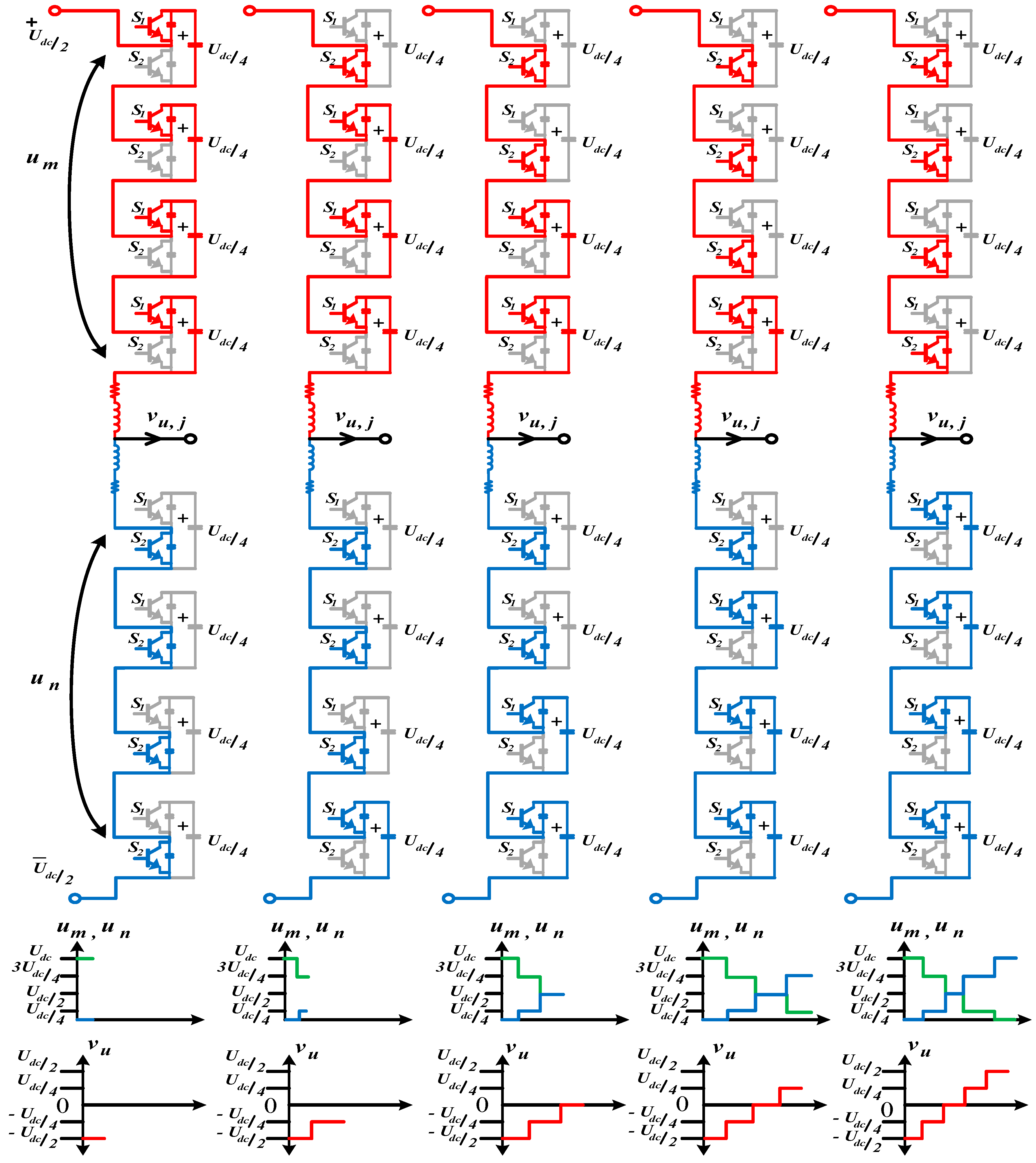
The insertion or bypassing of N-SM will give, levels of output waveform at every phase of the MMC. Where N represents No of SM and M represents the levels of output wave form. The switching operation of a single phase MMC is illustrated in Figure 2, using a single line schematic diagram.
A DC voltage “” is applied at the input of the MMC. The switches are operating in reciprocal fashion in each SM relying on the position ON or OFF. The solid line shows the capacitor is inserted and the dim line shows a capacitor is bypassed in every SM. The insertion and bypassing of the capacitor will define different levels of voltage at its terminal shown in Figure 2. The capacitor state that is inserted or bypassed are summarized in Table 1.
2.2. System Mathematical Modeling
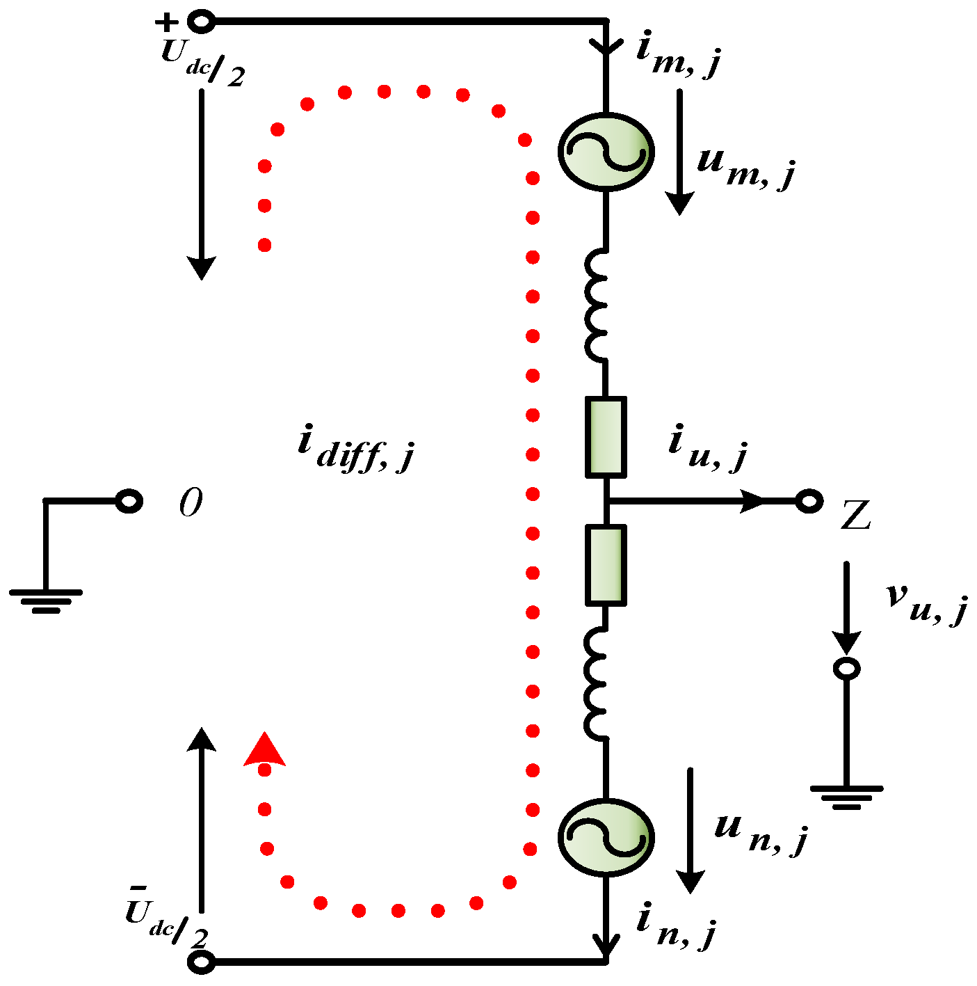
The mathematical modeling of the MMC is derived from a single-phase equivalent circuit as shown in Figure 3.
By applying the Kirchhoff loop law, the relations for the arm voltages, output current, and circulating current of the converter are obtained as follow [34]. Where j ϵ {a, b, c}
where and denote arm inductance and arm resistance respectively. represent the entire DC bus terminal voltage. represent output voltage of converter at point Z. and represents submodule arm voltages. The upper arm is represented by subscript while a lower arm is represented by subscript . Different currents of the MMC are given as
where and represents the upper arm current and lower arm current. represent the output current. represents an internal circulating current. Adding and subtracting (1) and (2) we obtain the following relation.
The is internal voltage in (7), while in (8) is the internal unbalanced voltage of an MMC, and the internal over phase j ϵ {a, b, c} can be express as
where is the dc link current and supposed to be distributed equally in all phases. As a result, the circulating current described in (6) contains 1/3 of the DC link current and is the AC component of circulating current. The dynamics of an MMC are characterized in Equations (7) and (8). By evaluating Equation (7), the output current can be controlled by . Similarly, by evaluating Equation (8), the internal circulating current can be controlled by . Furthermore, the capacitor SM internal dynamics with regards to arm voltages and currents are expressed as
The capacitance of an SM capacitor is expressed by C, the number of SM in each half arm is represented by N, while capacitor sum voltages in upper and lower arms are represented by and . Insertion indices of upper and lower arms are represented by and . Insertion indices and equal to one means the SM capacitor is inserted while insertion indices and equal to zero means the SM capacitor is bypassed in corresponding arms. As stated by Equations (8) and (9), the reference calculated for the arm voltages can be expressed as
In (13) the is calculated from the internal loop current controllers [35], while is calculated from the circulating current eliminating controller, which can be used to minimize the three-phase circulating current in an MMC. It can be concluded from Equations (1), (2), (12), and (13) that and could be controlled by manipulating and , respectively.
3. Control Scheme of the MMC
3.1. Adaptive PI Controller Design
The adaptive PI is a hybrid controller in which fuzzy logic (FL) is used to update the gains of PI for a wide range of operation. The FL makes the processing operation of a PI controller easy in a non-linear system where the system is ill-defined and mathematically poorly designed. The FL pre-processes the controller input (I/P) signal and PI post-process error signal to get the desired output response from the plant.
3.1.1. Fuzzy Controller Architecture
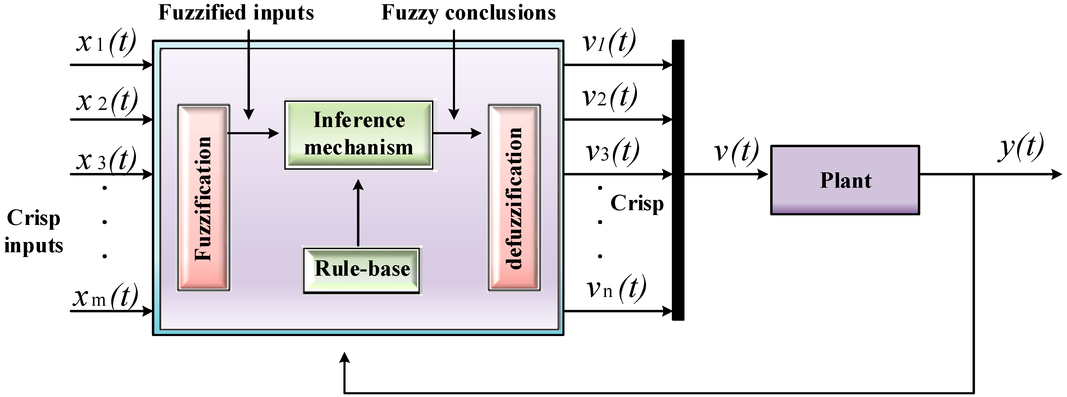
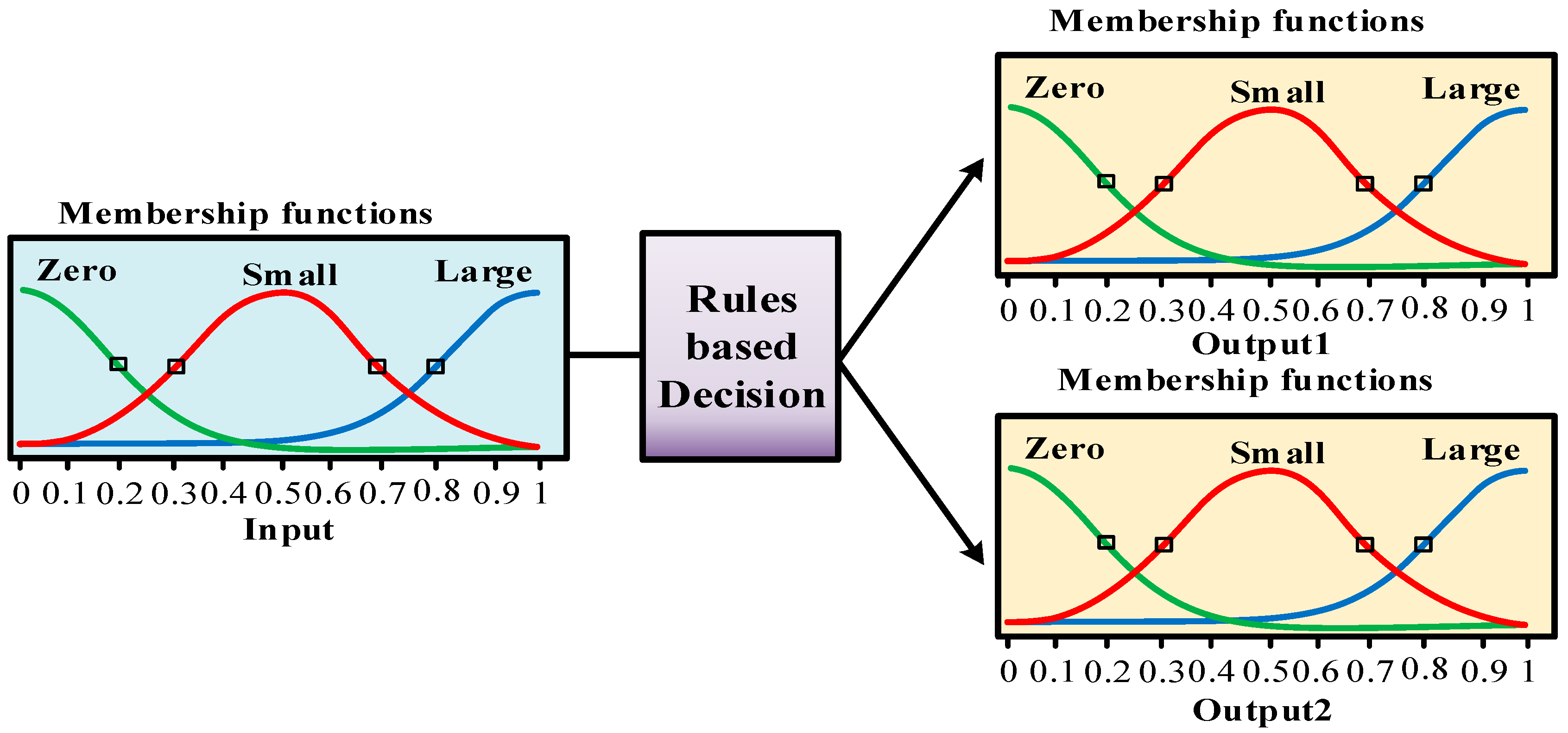
In the real world, problems related to a control system are largely complex, particularly when implementation problems are considered. The promising aspect of the fuzzy logic controller (FLC) is that they incorporate expert knowledge instead of entirely depending upon the exact mathematical model. Moreover, heuristics and intuition knowledge are also incorporated into the control system. Thus, FLC is suitable in applications, where models are ill-defined, not reliable enough, and complex. Essentially, the FLC is an artificial decision maker who works in a closed-loop fashion in real-time as shown in Figure 4. It collects plant O/P information y(t), matches it with the reference I/P x(t), and decides what the plant I/P v(t) would be to assure performance objectives. The FLC is mainly composed of four main phases: rule-base, inference mechanism, fuzzification, and de-fuzzification.
- The “rule-base” which contains the information of controlling output variables are created in FLC, in the shape of IF-THEN rules, with condition and conclusion.
- The rules are evaluated in the inference mechanism according to the error. During inference mechanism, it is concluded which control rules are appropriate at the current situation. Moreover, the choice of I/P to the plant are also enabled in this phase.
- During the fuzzification, a “crisp” (which are real numbers, not fuzzy sets) or actual time information are collected and reshaped to a fuzzy set using fuzzy expressive terms, expressive variables, and membership functions. Moreover, I/P is modified and interpreted which are then compared with the rules defined in the rule-base.
3.1.2. Fuzzy PI Controller
The PI controller has tuning gains parameter and , respectively. The desired performance of PI control structure is improved by updating the gains, according to error . The adaptability is attained by employing fuzzy rules, as given below and graphically illustrated in Figure 5.
- If error is zero, then proportional gain is large and integral gain is small
- If error is small, then proportional gain is large and integral gain is zero.
- If error is large, then proportional gain is large and integral gain is large.
The “crisp inputs” in the form circulating current and output current are fuzzified and shaped to a fuzzy set using membership function. The fuzzy set is evaluated in the rules-base with condition and conclusion, and concludes which rules are appropriate at the current time. The defuzzification process involves the conversion of the fuzzy outcomes to circulating and output voltages utilizing the membership function. The fuzzy rule selected from the set is defuzzified by using the center of gravity method. While the Gaussian membership function (GMF) is used for fuzzification, the GMF uses two variables, variance or standard deviation and center as:
The defuzzified output of fuzzy is fed as a gain to PI. Thus, the PI controller for controlling the is mathematically defined as:
The PI controller for controlling the is mathematically defined as:
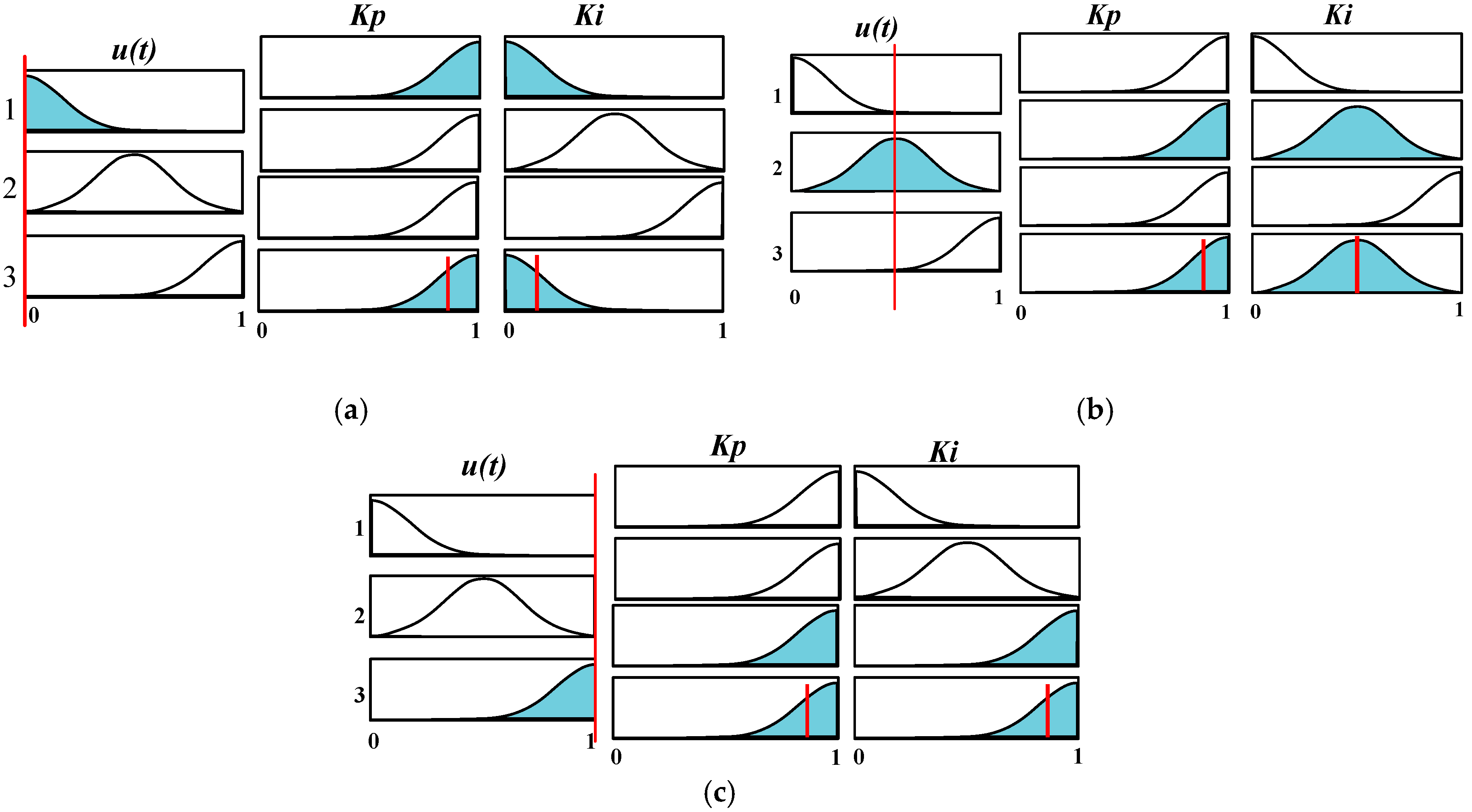
Whereas is controller input, and , controller outputs, and are controller gains respectively. However, the gain’s parameters of a conventional PI controller are constant in (15) and (16), which needs adaptation according to system load disturbance, parameter uncertainties, electrical faults, and load variations. To achieve adaptation, the designed controller use signal as an input for self-tuning of gain parameters, i.e., , respectively. Fuzzy IF-THEN rules are made as presented in Table 2. Based on these rules, a decision is performed by the inference engine. The defuzzified output is obtained by the center of gravity method for U1 and U2.
During fuzzification, the error signal, , information is collected and converted/fuzzified to fuzzy set using fuzzy linguistic terms and membership functions and compared with the IF-THEN rules defined in the rule-base. The rules are analyzed in the inference mechanism that decides the firing of the dominant rule. The fuzzy outcomes in the shape of and are obtained during defuzzification using the center of gravity method and update the gain parameters and , respectively. The rules employed in rule-base can be graphically illustrated in Figure 6a–c and shows the various scenarios in which U1 and U2 are actually computed by the fuzzy controller based on the absolute error. The line indices which corresponds to inputs can be moved to adjust gains as shown in Figure 6a–c.
So, the adaptation of (15) using the API controller for controlling is mathematically defined as
The adaptation of (16) using the API controller for controlling is mathematically defined as
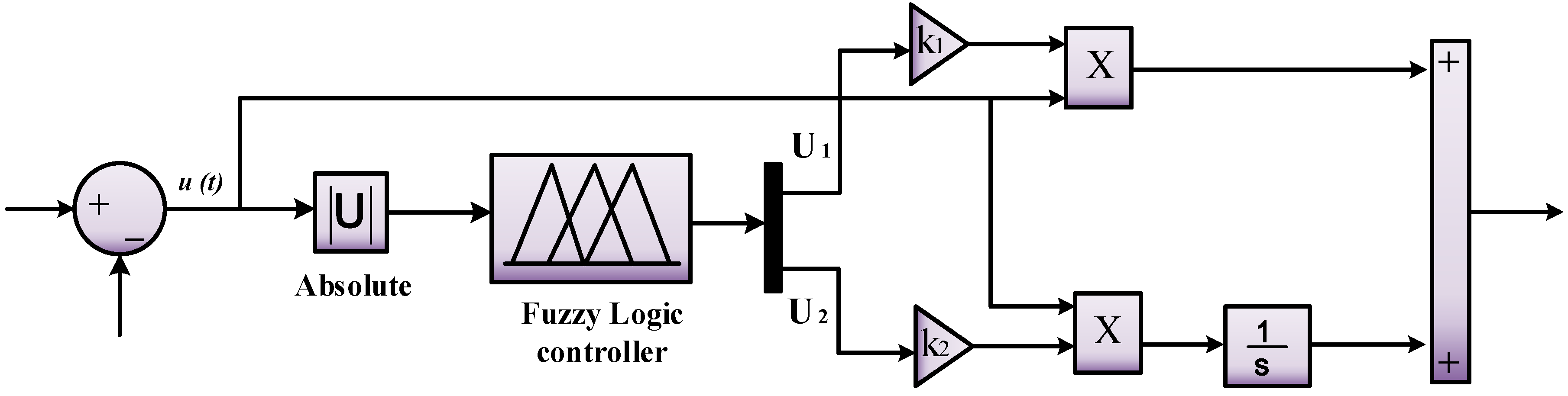
Whereas and are the fuzzy controller output for the gains and respectively. While and are used for the representation of updated gains and as shown in Figure 7.
3.2. Circulating Current Control
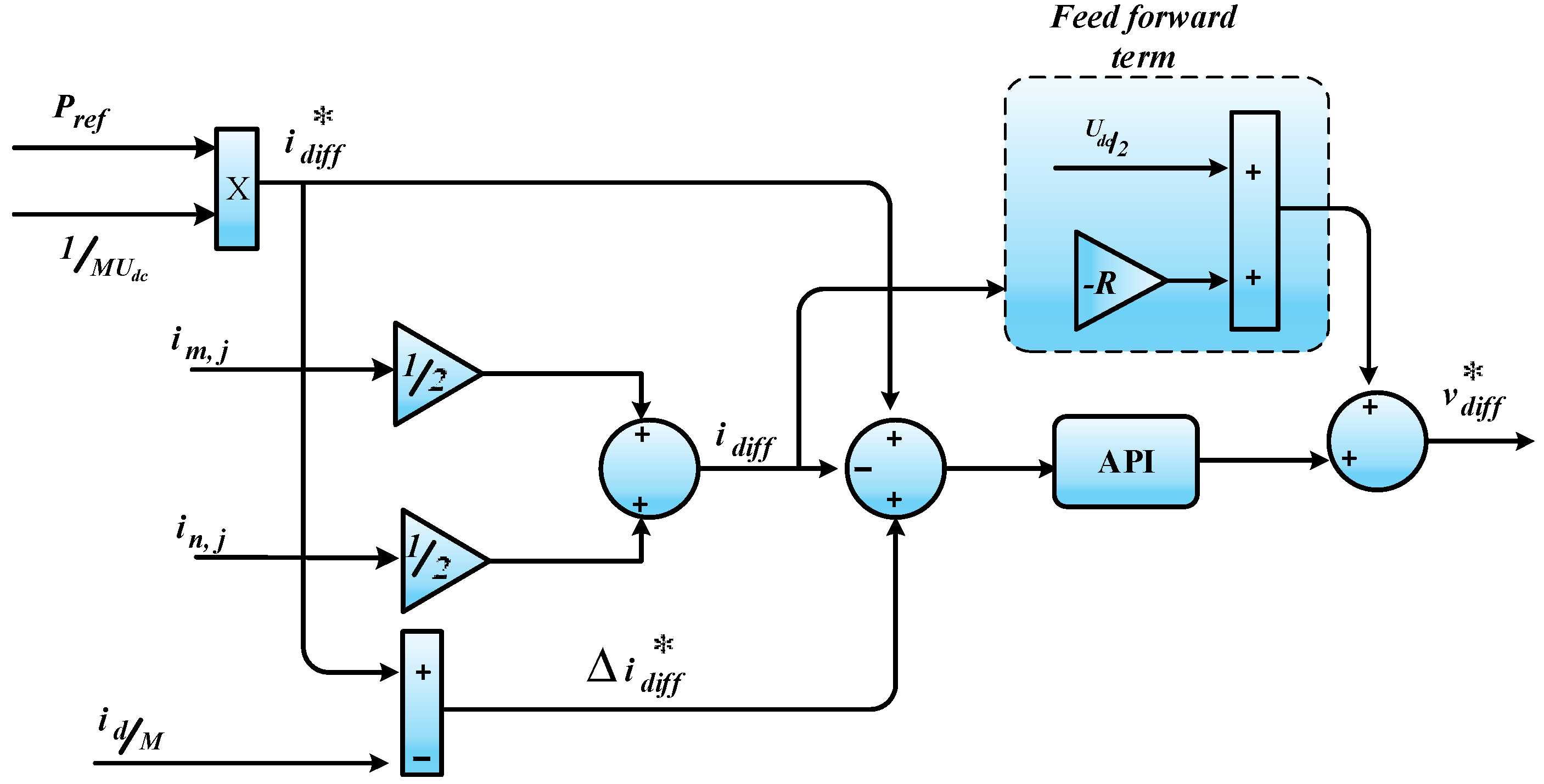
The can be regulated by , therefore, a control scheme is needed to regulate for controlling to overcome the converter losses. The variable is obtained through (8). A feedforward part is added to compensate the voltage drop. Filtering of is not required due to the lower number of harmonics in DC voltage compared to AC voltage. The control law we obtain
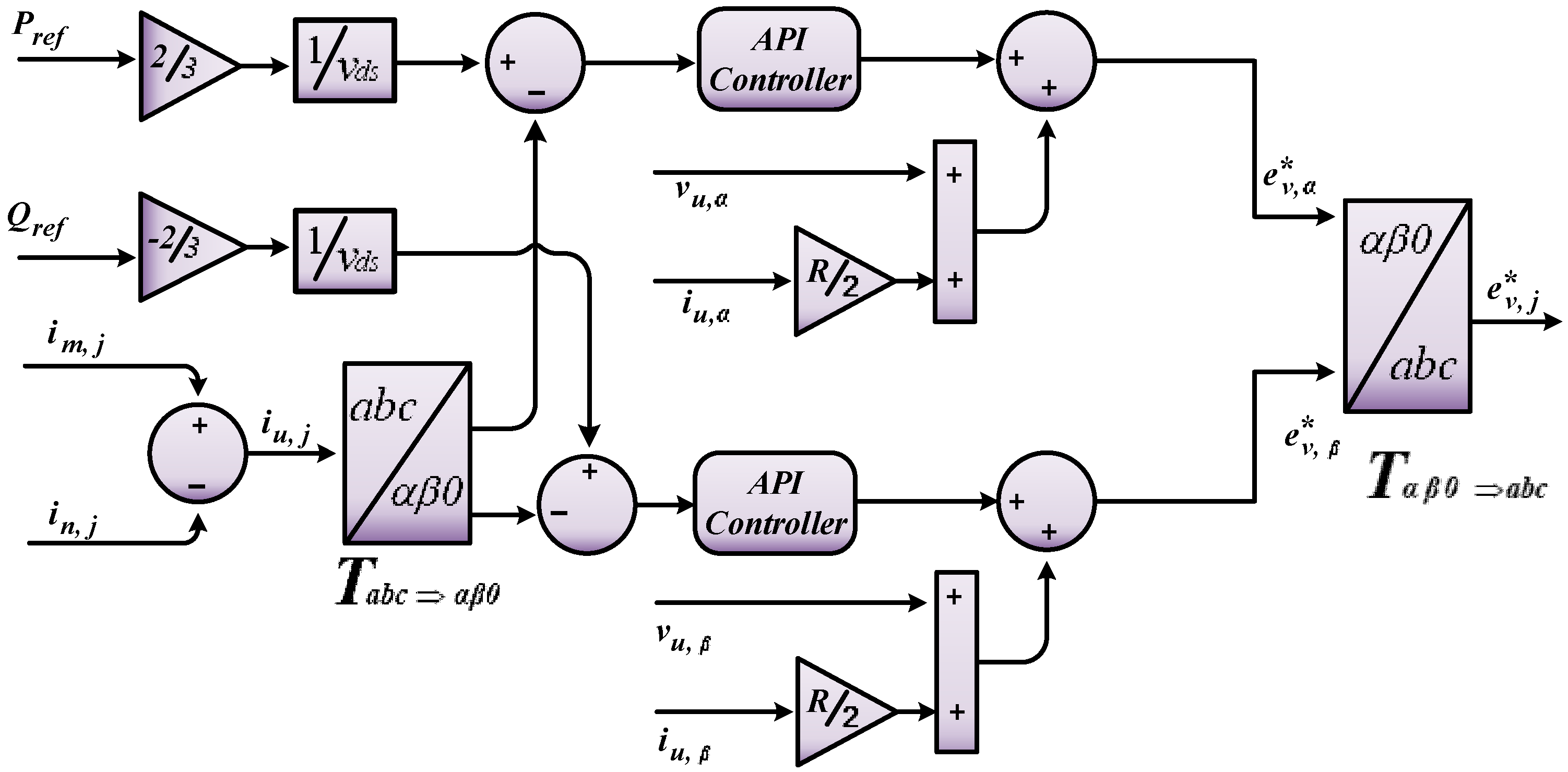
The reference is forced to get the desired value of circulating current, i.e., . The control structure using the API controller is shown in Figure 8.
3.3. Output Current Control
The output current can be regulated according to the following equation.
By evaluating (20), is the variable which can be regulated to control the output current . The Equation (20) can be rewritten as
Using the Clarke transformation Equation (20) can be transformed into axis from a-b-c frame .
For a three-phase balance system Equation (21) can be written
In control engineering usage is load disturbance which will vary inversely according to short circuit ratio [32]. Since is measurable by introducing a feedforward term, the dynamics can be improved. The control law obtained
where error control and the reference for voltage is computed using Equation (24), to control the output current. The output current control structure is shown in Figure 9.
The overall control scheme for controlling the circulating current and output current is shown in Figure 10.
4. Results and Discussions
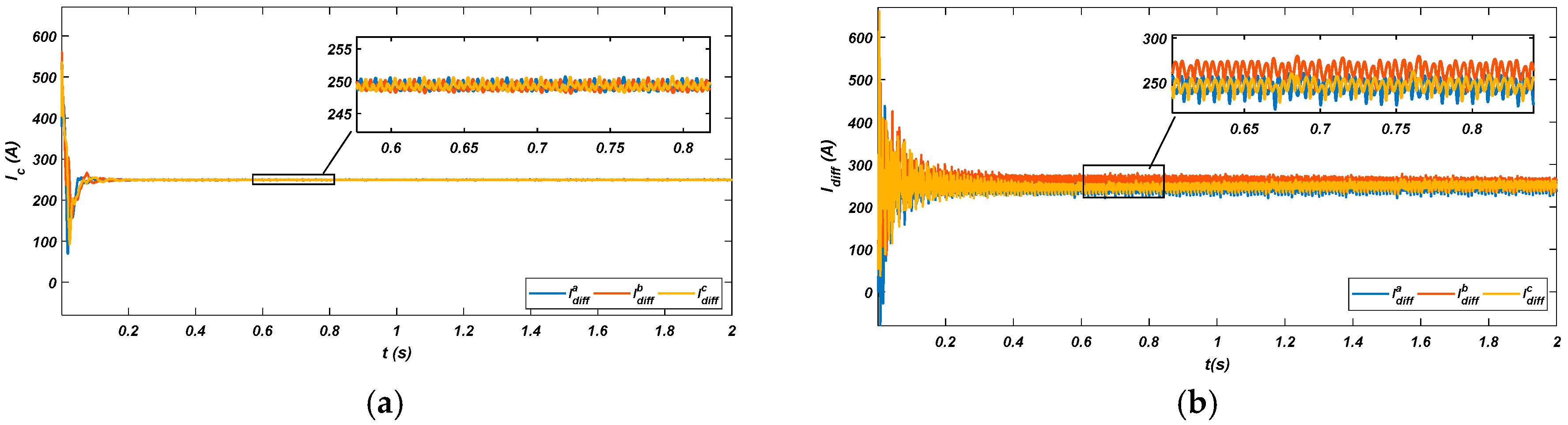
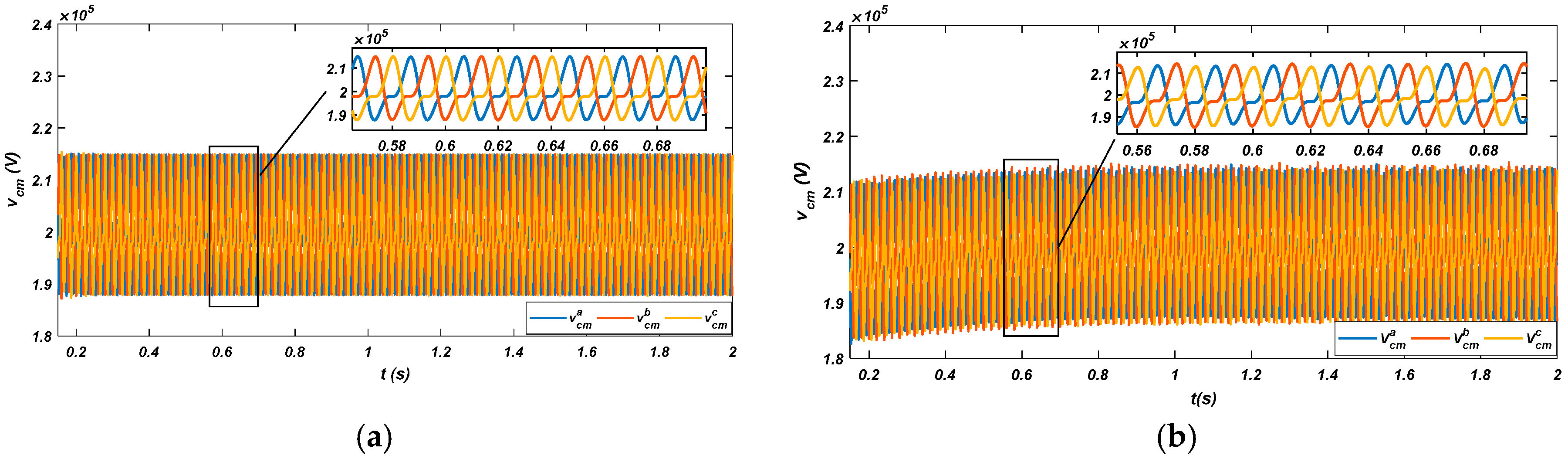
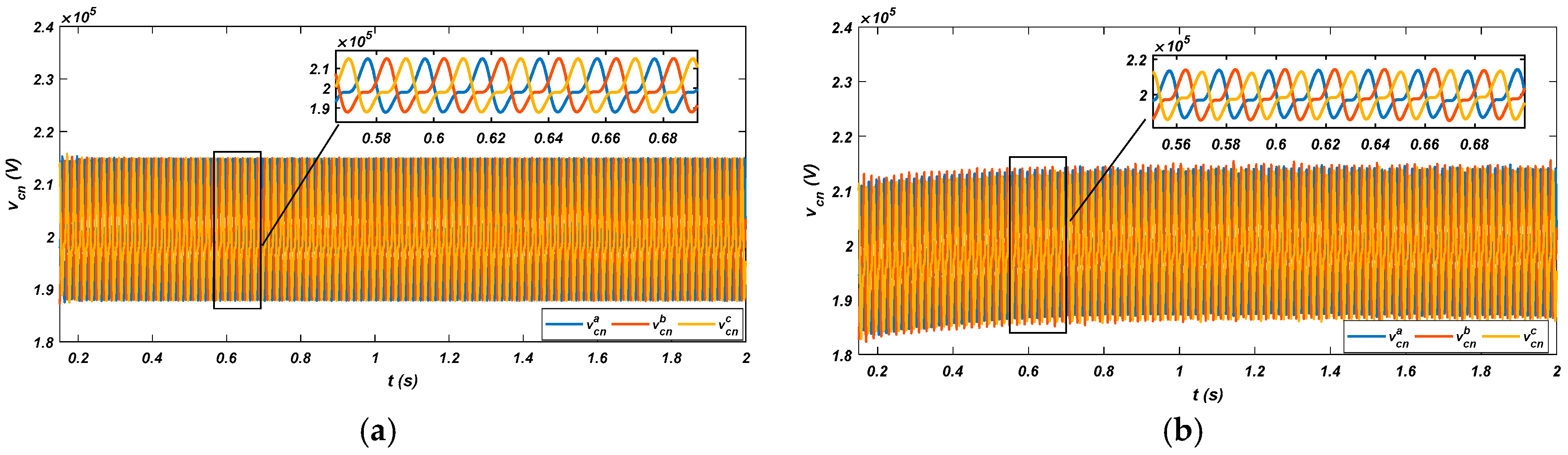
A control design architecture for a three-phase MMC model has been implemented with the help of MATLAB-Simulink (2017a, Natick, Massachusetts, MA, USA). The time for simulation is considered as 2 s. For better understanding, all the results are magnified. A comparative analysis of the results between the proposed API controller and a conventional PR controller has been made. The capacitor sum voltage and circulating current are the variables which need to be controlled, to reduce MMC losses. Ideally, the circulating current value should converge to DC input power, i.e., . The results of circulating current in Figure 11a,b is compared using the API and a PR controller. For a better understanding, the results are magnified for time t = 0.6 s to t = 0.8 s using the magnification tool. The API controller result shows that the circulating current value is converging to the desired value, i.e., 250 A with no oscillations during 0.2 s, showing good result compared to the PR controller. While in the case of PR controller the circulating current value is not converging to the desired value i.e., 250 A and also shows oscillations up to 0.2 s. Which means that the circulating current is not converged properly. It is also noted that circulating current one phase is exceeding the desired value, i.e., 250 A throughout the simulation as depicted in Figure 11b. The capacitor sum voltage average value should converge to DC link voltage mean value, i.e., to get a balance distribution of capacitor sum voltage over desired SM. The capacitor sum voltage of both an upper and a lower arm using the API and a PR controller are analyzed in Figure 12a,b and Figure 13a,b. For a better explanation, the results are magnified for time t = 0.58 s to t = 0.68 s using the magnification tool. The API controller display proper convergence of capacitor sum voltage to a desired DC link mean value for both upper and lower arm. All phase voltages are balanced in magnitude, which shows the balance distribution of capacitor sum voltage for the required SM in both upper and lower arm. As opposed to the API controller, the capacitor sum voltage of both upper and lower arms using the PR controller showed an imbalance in magnitude and created a trajectory path from 0.2 s to 0.8 s, which meant that the capacitor sum value was not totally converged to the desired DC link mean value for a balanced distribution of capacitor voltage in the required SM.
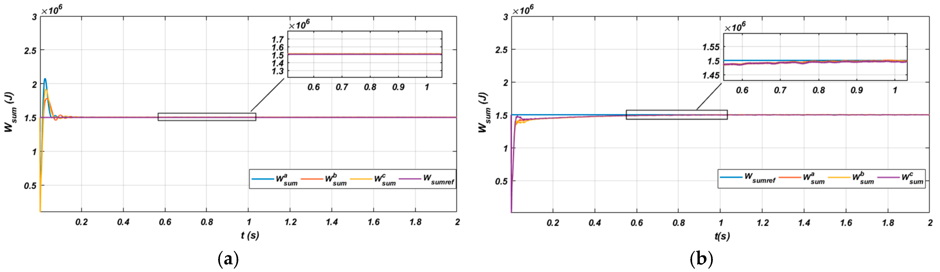
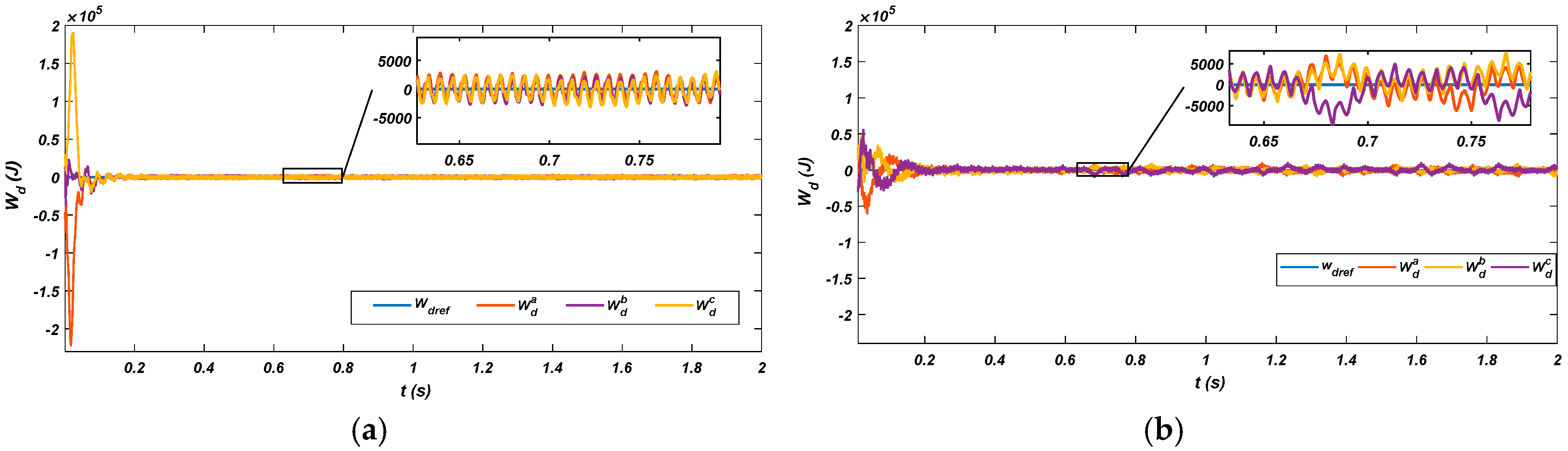
The dynamics of sum energy for both controllers are shown in Figure 14a,b. For better analysis, the results are magnified for time t = 0.6 s to t = 1 s using the magnification tool. At the start, the API controller shows overreaction. The rules defined in the rule-base are called and the decision is carried out to fire the dominant rule. The API controller takes only 0.024 s to clear transient, and the reference is completely tracked at 0.75 s completely without further overshoot, undershoot, steady state error, and ripples. However, in the case of the PR controller, the reference is completely tracked at 1 s. Moreover, the API controller shows a fast and robust response during the transient state. While the sum energy using a PR controller shows slower, oscillatory, and steady-state error. Which means that the PR controller response is slower than the proposed API controller. The energy difference mean value should be regulated correctly and converged to the zero reference value properly. The energy difference dynamics of the MMC for both controllers are shown in Figure 15a,b. For the result analysis, the results are magnified using the magnification tool for t = 0.65 s to t = 0.8 s. At the start, the proposed API controller shows an overreaction for 0.012 s, because the gains parameters are not updated. The rules defined in the rule-base are recalled and update the gain parameters of the PI controller. Once the parameters are updated, the proposed controller start tracking the reference without any further overshoot and converges the delta energy properly to the desired mean value. However, in the PR controller, the delta energy mean value is not converged properly, or showing disturbance, during time interval 0.65 s to 0.8 s. Moreover, the energy difference of both controllers is nearly close to zero. However, the API controller shows perfectly close convergence to zero and oscillating between positive and negative values giving an average value of zero, which means that the energy difference is regulated correctly and converged to zero reference value properly. In comparison to the API, the PR controller in the zoomed window shows that the desired value is showing some disturbance from 0.6 s to 0.8 s, which means that value is not converging to zero correctly during the mentioned time frame or showing a steady state error.
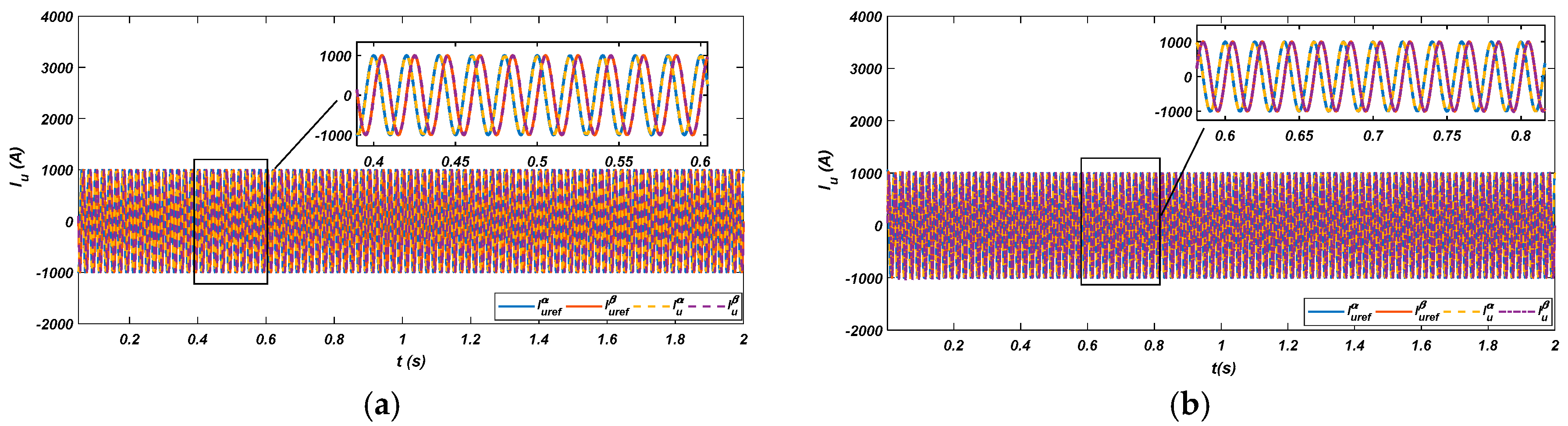
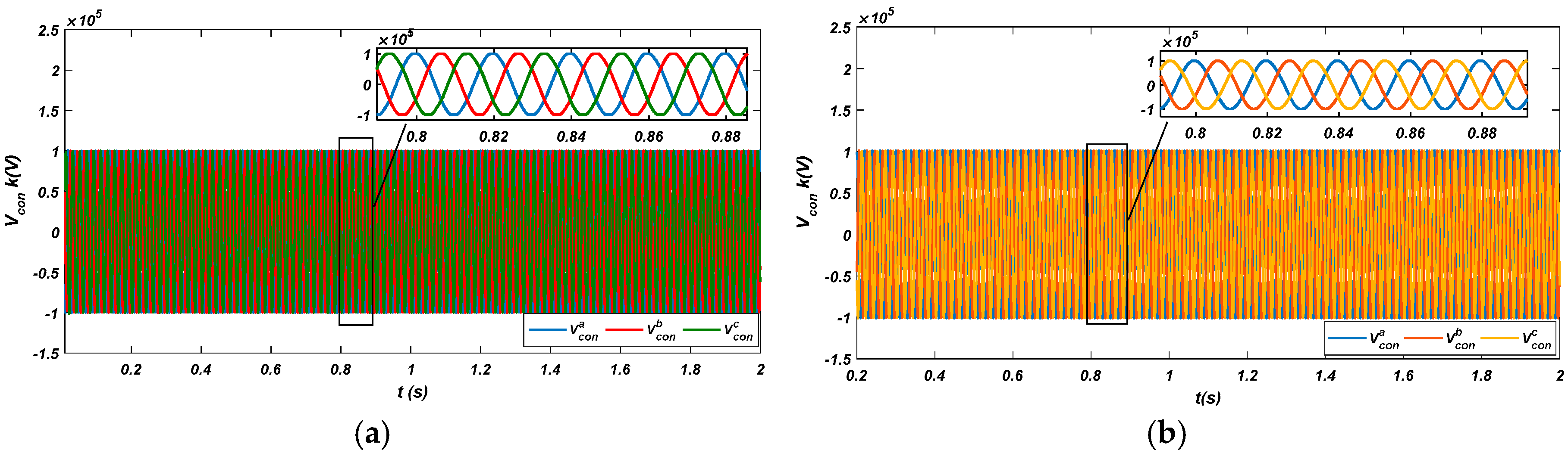
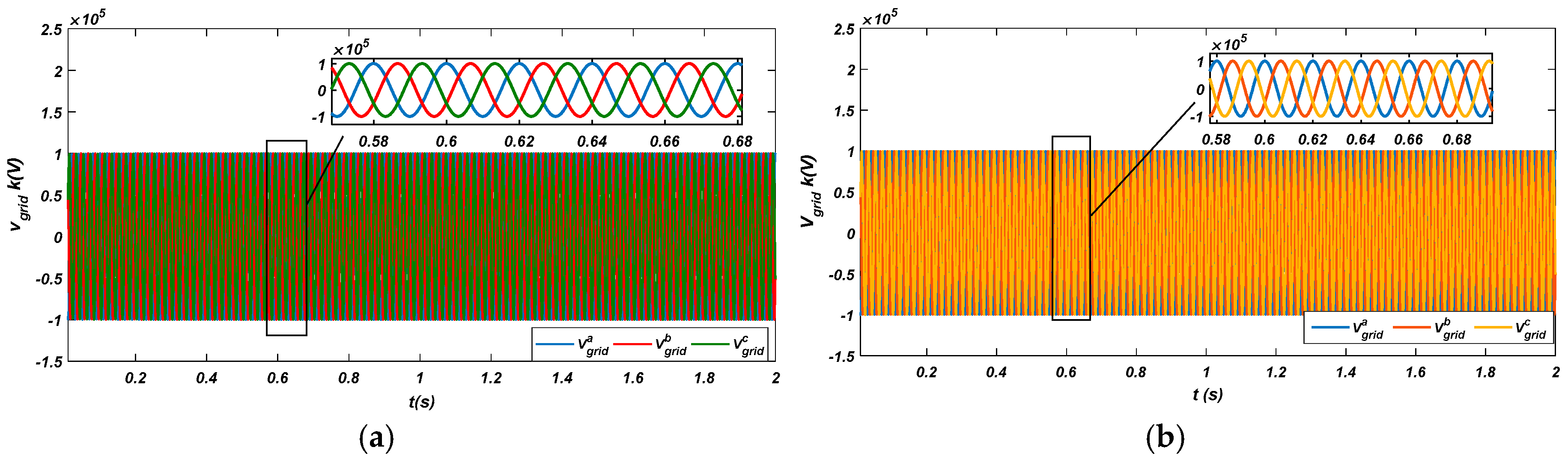
The output current is transformed in the αβ axis for both controllers shown in Figure 16a,b. For the explanation of results, the results are magnified using the magnification tool for t = 0.6 s to t = 0.8 s. For both controllers, the comparison is made on the basis of the performance indices, reference tracking, and transient and steady-state response. The API controller shows better performance indices, reference tracking, and transient and steady-state response compared to the PR controller. The performance indices are summarized in Table A2 of Appendix A, while converter and grid output phase voltages are shown in Figure 17a,b and Figure 18a,b for both controllers. For an explanation of the results, they are magnified using the magnification tool for t = 0.8 s to t = 0.88 s.
The control structure designed with the API controller is compared with conventional PR controller. The comparative analysis of a conventional PR and proposed API controller for controlling the output and circulating currents shows that the designed controller can track the references. The designed controller is also capable of converging the circulating current to the desired value. With the proposed control structure, the designed controller can converge the DC link voltage mean value to for the balance distribution of the capacitor sum voltage in the desired SM. The energy difference in both arms is well regulated by the proposed controller. The proposed API controller shows an improved transient response compared to the PR controller.
5. Conclusions and Future Work
This paper presents a control structure for controlling the circulating current and output current of the MMC during normal grid conditions. The control structure is implemented with an API controller. The control designed structure enables reference tracking, controlled circulating current, output current, the convergence of sum and delta energies to proper values. For validation of the proposed control structure, the results of the designed API controller are compared with a conventional PR control for verification.
MATLAB-Simulink results for both PR and API controllers shows that the API controller has a superior performance over the PR controller. The API controller can converge the circulating current to the desired value. The proposed API controller also shows improved transient response compared to the PR controller. In addition, the controller assures the reference tracking for sum energy and delta energy during the transient and steady response ensuring a stable three-phase output voltage. Moreover, the optimal performance achieved for the MMC parameters using the API controller are shown in Table A1 of Appendix A.
However, the designed control structure for circulating current and output current will be validated using FPGA or DSP TMS3200F28xx Kits (Texas Instruments, Dallas, TX, USA), Intel 8Xc196KC microcontroller (Intel corporation, Santa Clara, CA, USA) and dSPACE Digital Signal Controllers boards (DS1104, dSPACE Inc, Michigan, MI, USA). Feedback linearization and optimal control strategies will be designed and compared with conventionally tuned PR control structure.
Author Contributions
H.J.K., M.I., and W.U. conceptualized the main idea of this paper. M.I. implemented the mathematical equations, simulation verification, and the analyses. The paper was written by M.I. and reviewed by W.U., K.Z., S.U.I., I.K., and H.J.K. All authors were involved in formulating the final version of this paper. Furthermore, the work was supervised by H.J.K.
Funding
This research work was backed by BK21Plus, “the Creative Human Resource Development Program for IT Convergence”.
Conflicts of Interest
The authors declare no conflict of interest.
Appendix A

Table A1.
Converter parameters.
| Parameters | Values | Symbols | Units |
|---|---|---|---|
| D.C voltage | 200 | kV | |
| Grid voltage | 100 | kV | |
| Output current | 1 | kA | |
| Frequency | 50 | f | Hz |
| No of SM | 12 | N | - |
| Inductance | 50 | mH | |
| Resistance | 1.57 | Ω | |
| Capacitance | 0.45 | C | mF |
Table A2.
Performance indices evaluation.
| Performance Indices Elevation For | API Controller | PR Controller | ||||
|---|---|---|---|---|---|---|
| 1ISE | 2IAE | 3IATE | ISE | IAE | ITAE | |
| Circulating current | 3.714 | 0.2237 | 0.1834 | 1696 | 23.47 | 14.63 |
| 3.665 | 0.2105 | 0.1836 | 2247 | 25.46 | 14.47 | |
| 3.694 | 0.2200 | 0.1832 | 2483 | 25.31 | 25.31 | |
| Output current | 400.56 | 5.968 | 2.915 | 1022 | 13.5 | 8.913 |
| 20.86 | 5.658 | 2.997 | 50.5 | 13.1 | 9.009 | |
1ISE: Integral Square Error, 2IAE: Integral Absolute Error, 3ITAE: Integral of time Absolute Error.
References
- Marquardt, R. Modular Multilevel Converter: An universal concept for HVDC-Networks and extended DC-bus-applications. In Proceedings of the International Power Electronics Conference-ECCE ASIA-IPEC, Sapporo, Japan, 21–24 June 2010; pp. 502–507. [Google Scholar]
- Perez, M.A.; Bernet, S.; Rodriguez, J.; Kouro, S.; Lizana, R. Circuit topologies, modeling, control schemes, and applications of modular multilevel converters. IEEE Trans. Power Electron. 2015, 30, 4–17. [Google Scholar] [CrossRef]
- Li, Z.; Gao, F.; Xu, F.; Ma, X.; Chu, Z.; Wang, P.; Gou, R.; Li, Y. Power Module Capacitor Voltage Balancing Method for a ±350-kV/1000-MW Modular Multilevel Converter. IEEE Trans. Power Electron. 2016, 31, 3977–3984. [Google Scholar] [CrossRef]
- Akagi, H. Classification, terminology, and application of the modular multilevel cascade converter (MMCC). IEEE Trans. Power Electron. 2011, 26, 3119–3130. [Google Scholar] [CrossRef]
- Axelrod, B.; Berkovich, Y.; Ioinovici, A. A Medium-Voltage Motor Drive With a Modular. IEEE Trans. Power Electron. 2003, 3, 1786–1799. [Google Scholar]
- Parker, M.A.; Ran, L.; Finney, S.J. Distributed control of a fault-tolerant modular multilevel inverter for direct-drive wind turbine grid interfacing. IEEE Trans. Ind. Electron. 2013, 60, 509–522. [Google Scholar] [CrossRef]
- Gnanarathna, U.N.; Chaudhary, S.K.; Gole, A.M.; Teodorescu, R. Modular multi-level converter based HVDC system for grid connection of offshore wind power plant. In Proceedings of the 9th IET International Conference on AC and DC Power Transmission, London, UK, 19–21 October 2010; p. O53. [Google Scholar]
- Swetha, S.P.; Sumangala, B.V. Solar photovoltaic power conversion using modular multilevel inverter. In Proceedings of the International Conference on Emerging Research in Electronics, Computer Science and Technology (ICERECT), Mandya, India, 17–19 December 2015; pp. 387–391. [Google Scholar]
- Kenzelmann, S.; Rufer, A.; Dujic, D.; Canales, F.; de Novaes, Y.R. A versatile DC/DC converter based on modular multilevel converter for energy collection and distribution. In Proceedings of the IET Conference on Renewable Power Generation, Edinburgh, UK, 6–8 September 2011; p. 71. [Google Scholar]
- Mohammadi, H.P.; Bina, M.T. A transformerless medium-voltage STATCOM topology based on extended modular multilevel converters. IEEE Trans. Power Electron. 2011, 26, 1534–1545. [Google Scholar]
- Teeuwsen, S.P. Simplified dynamic model of a voltage-sourced converter with modular multilevel converter design. In Proceedings of the IEEE/PES Power Systems Conference and Exposition, Seattle, WA, USA, 15–18 March 2009; pp. 1–6. [Google Scholar]
- Münch, P.; Liu, S.; Dommaschk, M. Modeling and current control of modular multilevel converters considering actuator and sensor delays. In Proceedings of the 35th Annual Conference of IEEE Industrial Electronics, Porto, Portugal, 3–5 November 2009; pp. 1633–1638. [Google Scholar]
- Nademi, H.; Das, A.; Norum, L. An analytical frequency-domain modeling of a Modular Multilevel Converter. In Proceedings of the 3rd Power Electronics and Drive Systems Technology (PEDSTC), Tehran, Iran, 15–16 February 2012; pp. 86–91. [Google Scholar]
- Song, Q.; Liu, W.; Li, X.; Rao, H.; Xu, S.; Li, L. A steady-state analysis method for a modular multilevel converter. IEEE Trans. Power Electron. 2013, 28, 3702–3713. [Google Scholar] [CrossRef]
- Gnanarathna, U.N.; Gole, A.M.; Jayasinghe, R.P. Efficient modeling of modular multilevel HVDC converters (MMC) on electromagnetic transient simulation programs. IEEE Trans. Power Deliv. 2011, 26, 316–324. [Google Scholar] [CrossRef]
- Ilves, K.; Antonopoulos, A.; Norrga, S.; Nee, H.P. Steady-state analysis of interaction between harmonic components of arm and line quantities of modular multilevel converters. IEEE Trans. Power Electron. 2012, 27, 57–68. [Google Scholar] [CrossRef]
- Marquardt, R. Stromrichterschaltungen Mit Verteilten Energiespeichern. German Patent DE10103031A1, 24 January 2001. [Google Scholar]
- Siemaszko, D.; Antonopoulos, A.; Ilves, K.; Vasiladiotis, M.; Ängquist, L.; Nee, H.P. Evaluation of control and modulation methods for modular multilevel converters. In Proceedings of the International Power Electronics Conference-ECCE ASIA, Sapporo, Japan, 21–24 June 2010; pp. 746–753. [Google Scholar]
- Hagiwara, M.; Akagi, H. PWM control and experiment of modular multilevel converters. In Proceedings of the IEEE Power Electronics Specialists Conference, Rhodes, Greece, 15–19 June 2008; pp. 154–161. [Google Scholar]
- Gemmell, B.D.; Dorn, J.; Retzmann, D.; Soerangr, D. Prospects of multilevel VSC Technologies for power transmission. In Proceedings of the IEEE/PES Transmission and Distribution Conference and Exposition, Chicago, IL, USA, 21–24 April 2008; pp. 1–16. [Google Scholar]
- Rodríguez, J.; Lai, J.S.; Peng, F.Z. Multilevel inverters: A survey of topologies, controls, and applications. IEEE Trans. Ind. Electron. 2002, 49, 724–738. [Google Scholar] [CrossRef]
- Glinka, M.; Marquardt, R. A new AC/AC multilevel converter family. IEEE Trans. Ind. Electron. 2005, 52, 662–669. [Google Scholar] [CrossRef]
- Tu, Q.; Xu, Z.; Huang, H.; Zhang, J. Parameter design principle of the arm inductor in modular multilevel converter based HVDC. In Proceedings of the International Conference on Power System Technology, Hangzhou, China, 24–28 October 2010; pp. 1–6. [Google Scholar]
- Tu, Q.; Xu, Z.; Xu, L. Reduced Switching-frequency modulation and circulating current suppression for modular multilevel converters. IEEE Trans. Power Deliv. 2011, 26, 2009–2017. [Google Scholar]
- Hagiwara, M.; Akagi, H. Control and Experiment of Pulsewidth-Modulated Modular Multilevel Converters. IEEE Trans. Power Electron. 2009, 24, 1737–1746. [Google Scholar] [CrossRef]
- Bahrani, B.; Debnath, S.; Saeedifard, M. Circulating Current Suppression of the Modular Multilevel Converter in a Double-Frequency Rotating Reference Frame. IEEE Trans. Power Electron. 2016, 31, 783–792. [Google Scholar] [CrossRef]
- Perez, M.A.; Lizana, F.R.; Rodriguez, J. Decoupled current control of modular multilevel converter for HVDC applications. In Proceedings of the IEEE International Symposium on Industrial Electronics, Hangzhou, China, 28–31 May 2012; pp. 1979–1984. [Google Scholar]
- Li, Z.; Wang, P.; Chu, Z.; Zhu, H.; Luo, Y.; Li, Y. An Inner Current Suppressing Method for Modular Multilevel Converters. IEEE Trans. Power Electron. 2013, 28, 4873–4879. [Google Scholar] [CrossRef]
- Yang, S.; Wang, P.; Tang, Y.; Zagrodnik, M.; Hu, X.; Tseng, K.J. Circulating Current Suppression in Modular Multilevel Converters With Even-Harmonic Repetitive Control. IEEE Trans. Ind. Appl. 2018, 54, 298–309. [Google Scholar] [CrossRef]
- Zhang, M.; Huang, L.; Yao, W.; Lu, Z. Circulating Harmonic Current Elimination of a CPS-PWM-Based Modular Multilevel Converter with a Plug-in Repetitive Controller. IEEE Trans. Power Electron. 2014, 29, 2083–2097. [Google Scholar] [CrossRef]
- He, L.; Zhang, K.; Xiong, J.; Fan, S. A Repetitive Control Scheme for Harmonic Suppression of Circulating Current in Modular Multilevel Converters. IEEE Trans. Power Electron. 2015, 30, 471–481. [Google Scholar] [CrossRef]
- Sharifabadi, K.; Harnefors, L.; Nee, H.P.; Norrga, S.; Teodorescu, R. Design, Control and Application of Modular Multilevel Converters for HVDC Transmission Systems, 1st ed.; John Wiley & Sons: West Sussex, UK, 2016; pp. 157–158. ISBN 9781118851562. [Google Scholar]
- Debnath, S.; Saeedifard, M. A New Hybrid Modular Multilevel Converter for Grid Connection of Large Wind Turbines. IEEE Trans. Sustain. Energy 2013, 4, 1051–1064. [Google Scholar] [CrossRef]
- Antonopoulos, A.; Angquist, L.; Nee, H.-P. On dynamics and voltage control of the Modular Multilevel Converter. In Proceedings of the 13th European Conference on Power Electronics and Applications, Barcelona, Spain, 8–10 September 2009; pp. 1–10. [Google Scholar]
- Tu, Q.; Xu, Z.; Zhang, J. Circulating current suppressing controller in modular multilevel converter. In Proceedings of the 36th Annual Conference on IEEE Industrial Electronics Society, Glendale, AZ, USA, 7–10 November 2010; pp. 3198–3202. [Google Scholar]
- Zeb, K.; Saleem, K.; Mehmood, C.A.; Uddin, W.; Ur Rehman, M.Z.; Haider, A.; Javed, M.A. Performance of adaptive PI based on fuzzy logic for Indirect Vector Control Induction Motor drive. In Proceedings of the 2nd International Conference on Robotics and Artificial Intelligence (ICRAI), Rawalpindi, Pakistan, 1–2 November 2016; pp. 93–98. [Google Scholar]
- Zeb, K.; Din, W.; Khan, M.; Khan, A.; Younas, U.; Busarello, T.; Kim, H. Dynamic Simulations of Adaptive Design Approaches to Control the Speed of an Induction Machine Considering Parameter Uncertainties and External Perturbations. Energies 2018, 11, 2339. [Google Scholar] [CrossRef]
Figure 1.
General MMC 3 phase structure.

Figure 2.
Switching operation of the single phase MMC.

Figure 3.
Single phase equivalent circuit.

Figure 4.
Fuzzy controller architecture to controlled plant.

Figure 5.
Output–input membership functions.

Figure 6.
Adaptation of gain values where the: (a) error is zero, (b) error is small, and (c) error is large.
Figure 6.
Adaptation of gain values where the: (a) error is zero, (b) error is small, and (c) error is large.

Figure 7.
Control structure for error tracking.

Figure 8.
Circulating current control.

Figure 9.
Output Current control.

Figure 10.
Overall control design for output and circulating currents.

Figure 11.
(a) Circulating current using the API controller; (b) circulating current using the PR controller.
Figure 11.
(a) Circulating current using the API controller; (b) circulating current using the PR controller.

Figure 12.
(a) Capacitor voltage of an upper arm using the API controller; (b) capacitor voltage of an upper arm using the PR controller.
Figure 12.
(a) Capacitor voltage of an upper arm using the API controller; (b) capacitor voltage of an upper arm using the PR controller.

Figure 13.
(a) Capacitor voltage of a lower arm using the API controller; (b) capacitor voltage of a lower arm using the PR controller.
Figure 13.
(a) Capacitor voltage of a lower arm using the API controller; (b) capacitor voltage of a lower arm using the PR controller.

Figure 14.
(a) Sum energy of arms using the API controller; (b) sum energy of arms using the PR controller.
Figure 14.
(a) Sum energy of arms using the API controller; (b) sum energy of arms using the PR controller.

Figure 15.
(a) Energy difference of arms using the API controller; (b) energy difference of arms using the PR controller.
Figure 15.
(a) Energy difference of arms using the API controller; (b) energy difference of arms using the PR controller.

Figure 16.
(a) Output current using the API controller; (b) output current using the PR controller.

Figure 17.
(a) Converter phase voltages using the API controller; (b) converter phase volatges using the PR controller.
Figure 17.
(a) Converter phase voltages using the API controller; (b) converter phase volatges using the PR controller.

Figure 18.
(a) Grid phase voltage using the API controller; (b) grid voltage using the PR controller.
Figure 18.
(a) Grid phase voltage using the API controller; (b) grid voltage using the PR controller.

Table 1.
Capacitor states.
| Scenario | Capacitors States in the Upper Arm | Capacitors States in the Lower Arm | Output Voltage |
|---|---|---|---|
| 1 | All capacitors are inserted | All capacitor bypassed | |
| 2 | One capacitor bypassed and three capacitors inserted | One capacitor inserted and three capacitors bypassed | |
| 3 | Two capacitors bypassed and two capacitors inserted | Two capacitors inserted and two capacitors bypassed | 0 |
| 4 | Three capacitors bypassed and one capacitor inserted | Three capacitors inserted and one capacitor bypassed | |
| 5 | Four capacitors bypassed and zero capacitors inserted | Four capacitors inserted and zero capacitors bypassed |
Table 2.
IF-THEN rules employed for gain adaptation.
| Input Membership Functions | IF-THEN Rules | Output Membership Functions | ||||
|---|---|---|---|---|---|---|
| S.No | Linguistic Terms | Range | If Input | Then Output ( | Linguistic Terms | Range |
| (1) | Zero | [0, 0.2] | Zero | Zero. Large | Zero | [0, 0.2] |
| (2) | Small | [0.3, 0.7] | Small | Large. Small | Small | [0.3, 0.7] |
| (3) | Large | [0.8, 1.0] | Large | Large. Large | Large | [0.8, 1.0] |
© 2019 by the authors. Licensee MDPI, Basel, Switzerland. This article is an open access article distributed under the terms and conditions of the Creative Commons Attribution (CC BY) license (http://creativecommons.org/licenses/by/4.0/).
Share and Cite
MDPI and ACS Style
Ishfaq, M.; Uddin, W.; Zeb, K.; Khan, I.; Ul Islam, S.; Adil Khan, M.; Kim, H.J. A New Adaptive Approach to Control Circulating and Output Current of Modular Multilevel Converter. Energies 2019, 12, 1118. https://doi.org/10.3390/en12061118
AMA Style
Ishfaq M, Uddin W, Zeb K, Khan I, Ul Islam S, Adil Khan M, Kim HJ. A New Adaptive Approach to Control Circulating and Output Current of Modular Multilevel Converter. Energies. 2019; 12(6):1118. https://doi.org/10.3390/en12061118
Chicago/Turabian StyleIshfaq, Muhammad, Waqar Uddin, Kamran Zeb, Imran Khan, Saif Ul Islam, Muhammad Adil Khan, and Hee Je Kim. 2019. "A New Adaptive Approach to Control Circulating and Output Current of Modular Multilevel Converter" Energies 12, no. 6: 1118. https://doi.org/10.3390/en12061118
Note that from the first issue of 2016, this journal uses article numbers instead of page numbers. See further details here.