Analysis of the Propagation Characteristic of Subsynchronous Oscillation in Wind Integrated Power System


1
State Grid Shaanxi Electric Power Research Institute, Xi’an 710100, China
2
School of Electrical & Electronic Engineering, North China Electric Power University, Changping District, Beijing 102206, China
*
Authors to whom correspondence should be addressed.
Energies 2019, 12(6), 1081; https://doi.org/10.3390/en12061081
Submission received: 9 January 2019
/
Revised: 10 March 2019
/
Accepted: 18 March 2019
/
Published: 20 March 2019
(This article belongs to the Special Issue Electrical Engineering for Sustainable and Renewable Energy)
Abstract
:This paper proposes oscillation propagation factors to analyze power oscillations caused by the interharmonics of doubly fed induction generators (DFIG) at different points in the power system. First, a dynamic model of the DIFG is built, including the asynchronous generator, its transmission system, converters and the control systems. Then, the state space expression is formed by deducing the input and output matrices. From this, the oscillation propagation factor is proposed and denoted to exhibit the propagation mechanism of interharmonics in the view of frequency domain, by deducing the multi-input-multi-output transfer functions matrix. Along with this, the sensitivity of propagation is calculated for adjusting the parameters to block the oscillation propagating path. Finally, the modified four machine system with two DFIGs and the New-England 39 bus system with two DFIGs is used as a test system to verify the effectiveness of the oscillation propagation factor. From this the simulation results demonstrate that the subsynchronous interharmonics of DFIGs injected into the grid will propagate to the different points of the system and results in oscillation of the power. The oscillation propagation factor could quantize the oscillation magnitude propagating from one point to other point in the wind integrated power system.
1. Introduction
New energy sources such as wind power and photovoltaic cells have become an important part of the power system. With the continuous increase of the proportion of new energy sources, the stability of the power system caused by the access of new energy has attracted wide attention [1,2,3]. Wind power is one of the best solutions for new energy generation [4]. At present, doubly fed induction generator (DFIG) and permanent magnet synchronous generator (PMSG) are the mainstream machine types for wind power generation [5]. In order to improve the stability and reliability of the wind integrated power system, it is necessary to make a much deeper study on the phenomenon of subsynchronous oscillation in the doubly-fed induction generation system.
The DFIG rotor-side converters and grid-side converters contain high power electronics. When the random variation of wind speed causes the frequency variation of the DFIG rotor excitation current, due to the switching effect during the conversion or regulation process, the rotor current frequency and the grid frequency will cause the subsynchronous frequency interharmonics in the DFIG current [6,7].
Reference [7] shows that the DFIG can act as a source of significant subsynchronous interharmonic current emissions. When the interharmonic current is injected into the grid, it will cause voltage, current and power to oscillate, causing various faults and the instability of the power system [8]. Subsynchronous oscillation caused by DFIG has been studied in terms of damping and impedance, such as eigenvalue analysis [9,10], frequency scanning method [11,12], and equivalent impedance [13,14,15]. References [9,10] analyze and control the subsynchronous oscillation based on eigenvalue analysis. Frequency scanning method is performed to investigate subsynchronous control interaction [11,12]. An impedance-based analysis approach is used to characterize subsynchronous oscillation [13,14,15]. At present, there is no literature to quantitatively study the propagation law of DFIG subsynchronous interharmonics.
The rest of the paper is structured as follows: Section 2 gives the dynamic model of DFIG. In Section 3, a small signal state space model for the power system is derived from the DFIG model, the synchronous generator state equation and the network equation considering the load. Then we calculate the system transfer function matrix and define the oscillation propagation factor to analyze the system power oscillation. Section 4 validates the effectiveness of the oscillation propagation factor based on the 4-machine 2-area system and the New-England 39 bus system. The discussion and conclusion are provided in Section 5 and Section 6 respectively.
2. Dynamic Model of Wind Integrated Power System
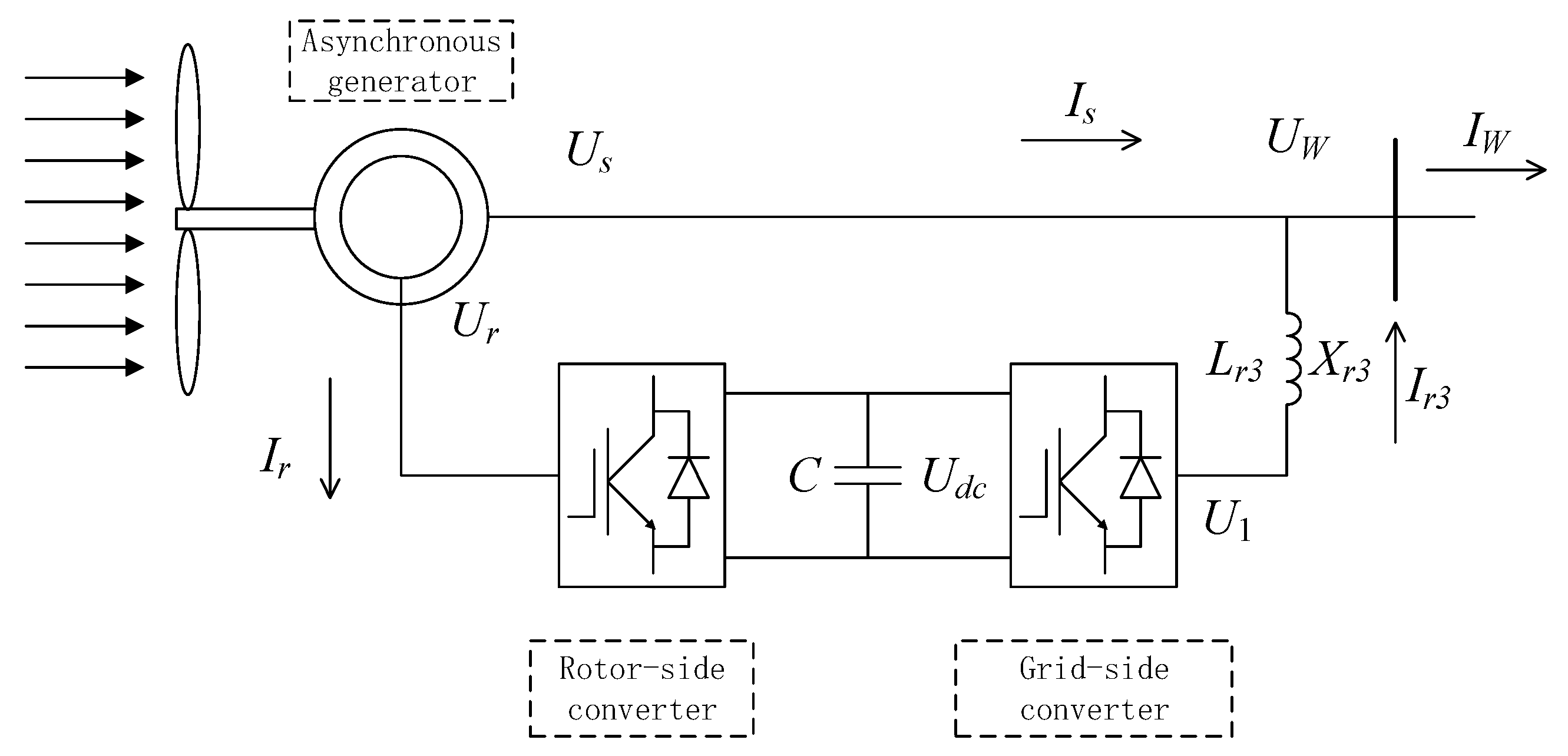
The doubly fed induction generator structure is shown in Figure 1. It mainly includes asynchronous generator, transmission system, rotor-side converter, grid-side converter and control system [16,17].
In Figure 1, is the stator voltage of DFIG, is the stator current; is the rotor voltage, is the rotor current; is the AC side voltage of the grid-side converter, and is the AC side current of the grid-side converter. is the filter between the AC side of the grid-side converter and the line. is the filter reactance. C is the capacitance value of the intermediate capacitor, and is the DC voltage of the capacitor. UW is the DFIG bus voltage; IW is the DFIG bus injection current. The positive direction of the physical quantity uses the generator convention.
Ignoring the transient process of the motor stator flux, according to the DFIG flux and voltage equations [16,18], the dynamic model of the asynchronous generator is (1).
where and are the d-axis and q-axis components of the stator transient voltage, respectively; and are the d-axis and q-axis components of the rotor winding voltage, respectively; and are the d-axis and q-axis components of the stator winding current, respectively; is the slip; is the rotor winding resistance; is the excitation reactance; , where is the rotor leakage reactance; is the inertia time constant of the whole drive; is the electromagnetic torque; is the mechanical torque; D is the damping coefficient; is the slip at steady state, is the synchronous angular frequency.
Considering the DC voltage dynamics, the dynamic model of the intermediate capacitor C in Figure 1 is:
where is the active power from the rotor-side converter to the intermediate capacitor; is the active power from the intermediate capacitor to the grid-side converter.
The dynamic model of the filtered reactance is:
where and , are the d-axis and q-axis components of the current on the AC side of the grid-side converter, respectively; and are the d-axis and q-axis components of the AC side voltage of the grid-side converter, respectively;
The control objective of the rotor-side converter is to achieve decoupling independent control of the active power and reactive power on the stator side by controlling the excitation voltage [19]. The control block diagram of the rotor-side converter is available from [17].
The dynamic model of the rotor-side converter is:
where , and are the introduced state variables; , and , are the integral coefficients of the corresponding PI controller; and are the active and reactive powers of the stator winding, respectively; and are the d-axis and q-axis components of the rotor winding current, respectively. The superscript * indicates the reference value of the corresponding physical quantity.
The control objective of the grid-side converter is to maintain the intermediate capacitor voltage as stable, and control the reactive power exchange between the rotor side and the grid to zero [20]. The control block diagram of the grid-side converter is available from [16].
The dynamic model of the grid-side converter is:
where , and are the introduced state variables; , and are the integral coefficients of the corresponding PI controller.
3. Oscillation Propagation Factor
3.1. The Linearization Model
The DFIG dynamic models (1)–(5) are linearized to obtain a small-signal model of DFIG:
In (6), is the DFIG state variable; is the DFIG bus voltage, and is the DFIG bus injection current.
According to (6), the mathematical model of all DFIGs in the wind integrated power system is (7).
where is the state matrix; is the input matrix; is the output matrix; is the direct transfer matrix; is the state vector; is the DFIG voltage vector; is the DFIG current vector; n is the number of DFIGs in wind integrated power system.
The synchronous generator and its excitation system use a fourth order model. The linearized synchronous generator state equation is (8).
where is the synchronous generator state vector; is the bus voltage vector of synchronous generator; is the synchronous generator injection current vector; , , and are state matrix, input matrix, output matrix, and direct transfer matrix, respectively.
The load uses the constant impedance model. The power network equation considering load is (9)
where , ; is the node admittance matrix considering the load.
By combining (7), (8) and (9), (10) can be obtained.
where , , , , .
The active power injected into the grid by DFIG is :
By linearizing (11), we get,
According to the mathematical model of DFIG, we get (13):
where is the transient reactance of DFIG. , is the stator leakage reactance. Substituting (13) into (12), the active power of DFIG can be written as (14).
By combining (9), (10) and (14), the small-signal state space model of the whole system can be obtained:
where is the output vector; k is the number of generators in wind integrated power system; is the input vector; is the state matrix; is the input matrix; is the output matrix; is the direct transfer matrix.
3.2. Oscillation Propagation Factor
The Laplace transform is performed on the (15) and the initial condition is considered to be zero:
Eliminate in (16), then the transfer function matrix between the output variable and the input variable is:
where is a matrix function. The matrix element represents the sinusoidal response from the jth element of the input variable to the ith element of the output variable. For the jth element of the input variable with angular frequency , the amplitude of the ith element of the output variable is , the phase shift is , and the total response is equal to the linear sum of the individual input responses:
After the DFIG interharmonics are injected into the grid, the resulting disturbances will respond at different points in the power system. In the multi-input-multi-output systems, we define oscillation propagation factors to characterize the effects of the input variable disturbances with different frequencies on the oscillations amplitude of the output variables. The oscillation propagation factor is the ratio of an element of the output vector to the input vector. The oscillation propagation factor of the ith element of the output variable is denoted and calculated by (19) [21].
In (19), the unit of is dB; is the magnitude of the ith element of the output vector and is the 2 norm of the input vector. The larger the oscillation propagation factor, the stronger is the influence of the system disturbance at this point, and the larger the amplitude of the output vector element oscillation. Equation (17) can be expressed as:
It can be seen that when the elements of the transfer function matrix do not have zero pole cancellation, the pole of the transfer function is the same as the eigenvalue of the system state matrix. Consider the zero-polar format of the transfer function :
Substitute into (21) and replace pole with the eigenvalue of the state matrix . Then, we obtain the magnification of the transfer function , that is the amplitude gain of output.
When the angular frequency of the input variable approaches the angular frequency of the system, the factor in the denominator of (21) decreases, so the amplification factor increases and the oscillation propagation factor becomes larger. And when , the smaller , that is, the smaller the damping ratio, the larger the oscillation propagation factor.
The sensitivity of oscillation propagation factor to system parameters is calculated as follows:
where is the oscillation propagation factor of generators; is the angular frequency; is the system parameters, such as the active power of the DFIGs and the PI controller parameters of these DFIGs. The sensitivity can be solved by perturbation theory. Sensitivity indicates the influence of system parameters changes on the system oscillation propagation factor. The positive and negative sensitivity reflects the increase and decrease of the oscillation propagation factor when the system parameters fluctuate. The magnitude of the sensitivity reflects the degree of influence of system parameters on the oscillation propagation factor.
4. Simulation Results and Analysis
In order to verify the validity of the oscillation propagation factor proposed in this paper, the propagation of the subsynchronous oscillation in the test system is analyzed by the oscillation propagation factor. When the interharmonic frequency is changed, and when the system damping ratio is changed, the oscillation propagation factor is calculated to compare the strength of the subsynchronous oscillation of each generator.
4.1. Two Area Four Machine System
The modified 4-machine 2-area system [22] with two DFIGs is shown in Figure 2. The DFIG parameters are listed below. Rotor winding resistance p.u. Excitation reactance p.u. Rotor leakage reactance p.u. Filter reactance p.u. Capacitance C = 13.29 p.u. Inertia time constant p.u. The small-signal stability analysis was performed on the system of Figure 2, and seven oscillation modes were obtained, as shown in Table 1. The active power of DFIGs and the input vector are in Table 1. Eigenvalues for each mode are given in the form , from which the frequencies and the damping ratios are derived. The real part of the system eigenvalue is negative, and the system is small-signal stable.
4.1.1. Frequency Domain Simulation Results
The interharmonic d and q axis components obtained by Park’s transformation [23] are sinusoidal, and the phase of the d-axis component lags behind the phase of the q-axis component . Therefore, the input is as shown in (24).
where is the amplitude of interharmonic; is the angular frequency of interharmonic.
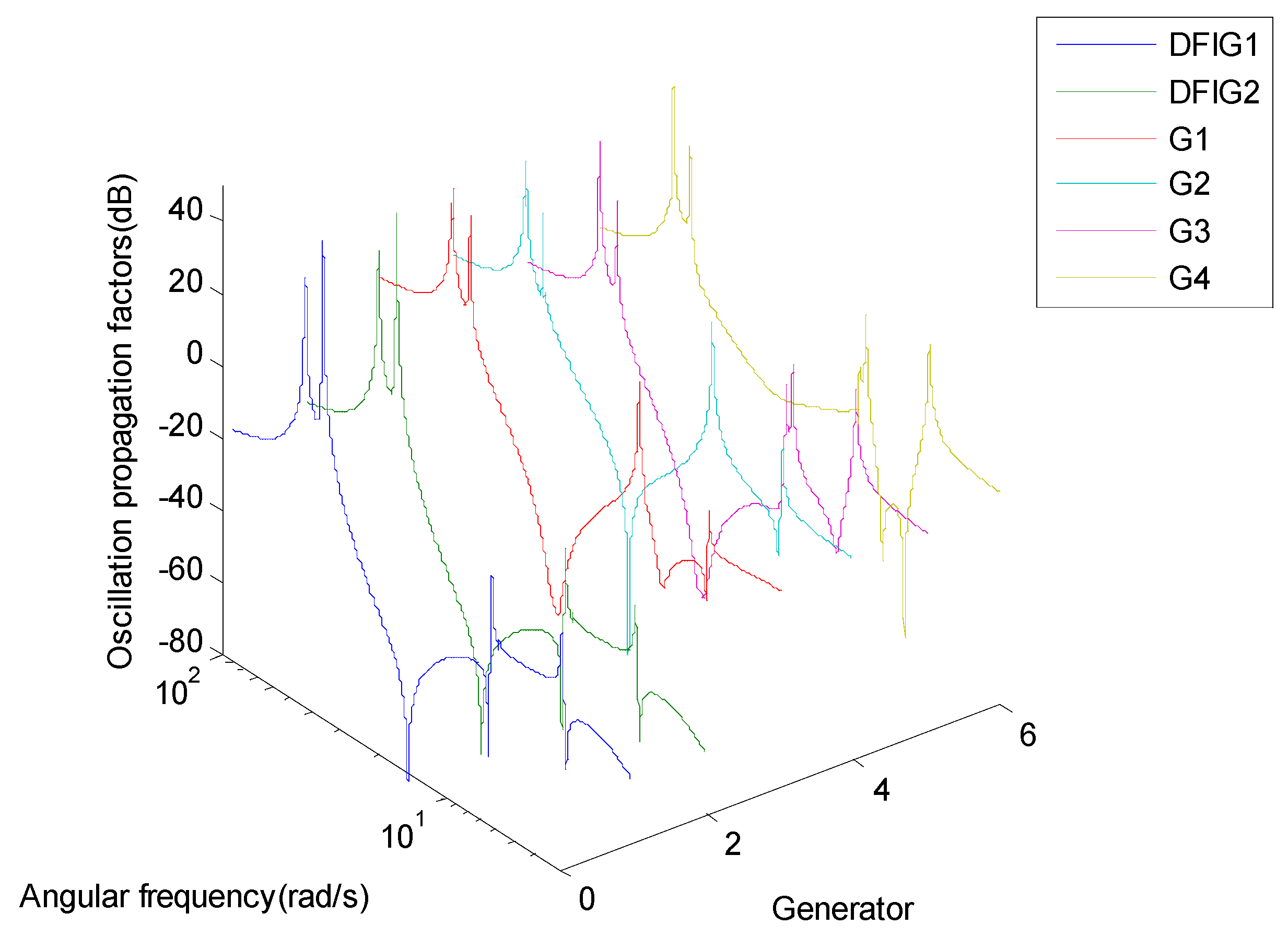
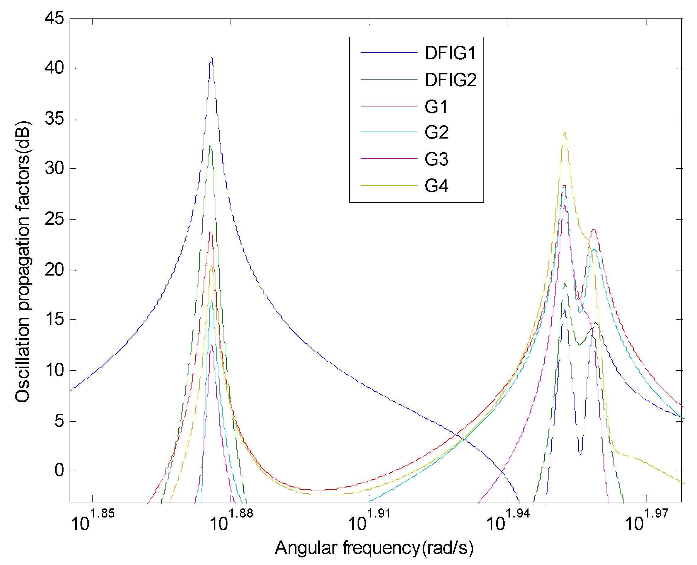
Assume interharmonic currents from DFIG1 is with the angular frequency of rad/s and amplitude of 0.001 p.u. is injected to the power grid. The output power of each DFIG and synchronous generator is taken as the output variable, and the system transfer function is established. The oscillation propagation factor is shown in Figure 3. Figure 4 shows the oscillation propagation factors for different generators near the oscillation frequency of system mode 1–4.
It can be seen from Figure 3 and Figure 4 that the oscillation propagation factors of the output power of the same generator are different for input variables of different angular frequency. When the angular frequency of the input variable is the same, the oscillation propagation factors of the output power of each generator are also different. When the input variable angular frequency is close to the oscillation angular frequency of system mode 1–4, the oscillation propagation factors of each generator exceed 0 dB, and the interharmonics of the DFIG are amplified by the system propagation. When the input variable frequency is close to the frequencies of mode 3 and 4, the amplitude of the output power oscillation of the DFIG is larger than the amplitude of the synchronous generator output power oscillation. When the input variable frequency is close to the frequencies of mode 1 and 2, the amplitude of the output power oscillation of the DFIG is smaller than the amplitude of the synchronous generator output power oscillation. The oscillation propagation factor of DFIG2 is given in Figure 5.
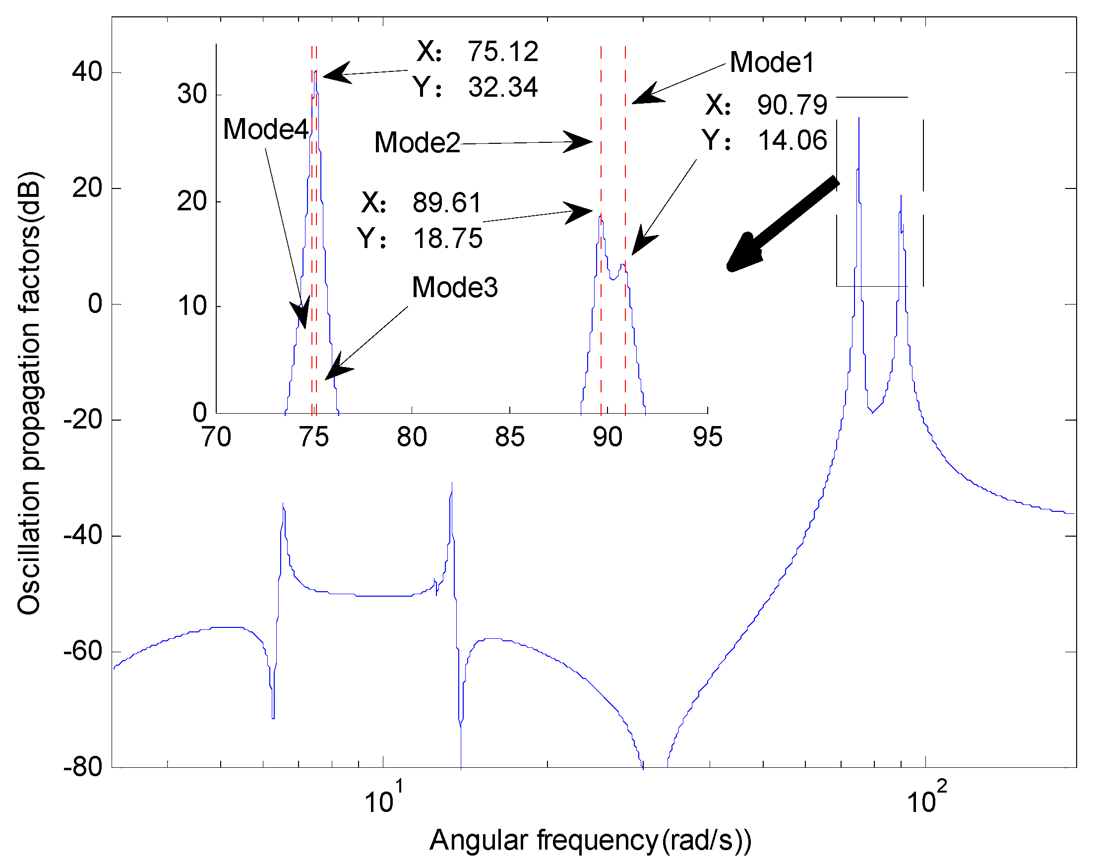
The abscissa of the red dotted line in Figure 5 is the system oscillation angular frequency. The abscissa of the three maximum points of the oscillation propagation factor of DFIG2 is 90.79 rad/s, 89.61 rad/s and 75.12 rad/s, respectively. These three angular frequency are almost equal to the system oscillation angular frequencies of mode 1, 2 and 3 in Table 1, respectively. When the inter-harmonics injected into the power network of the DFIG approaches these frequencies, resonance occurs, and a large amplitude power oscillation takes place. When the amplitude of the fluctuation of the inter-harmonic current becomes larger or smaller, the amplitude of the power oscillation also increases or decreases. The proportional relationship between the two amplitudes does not change, and corresponds to the ordinate value of the oscillation propagation factor characteristic curve at each frequency point.
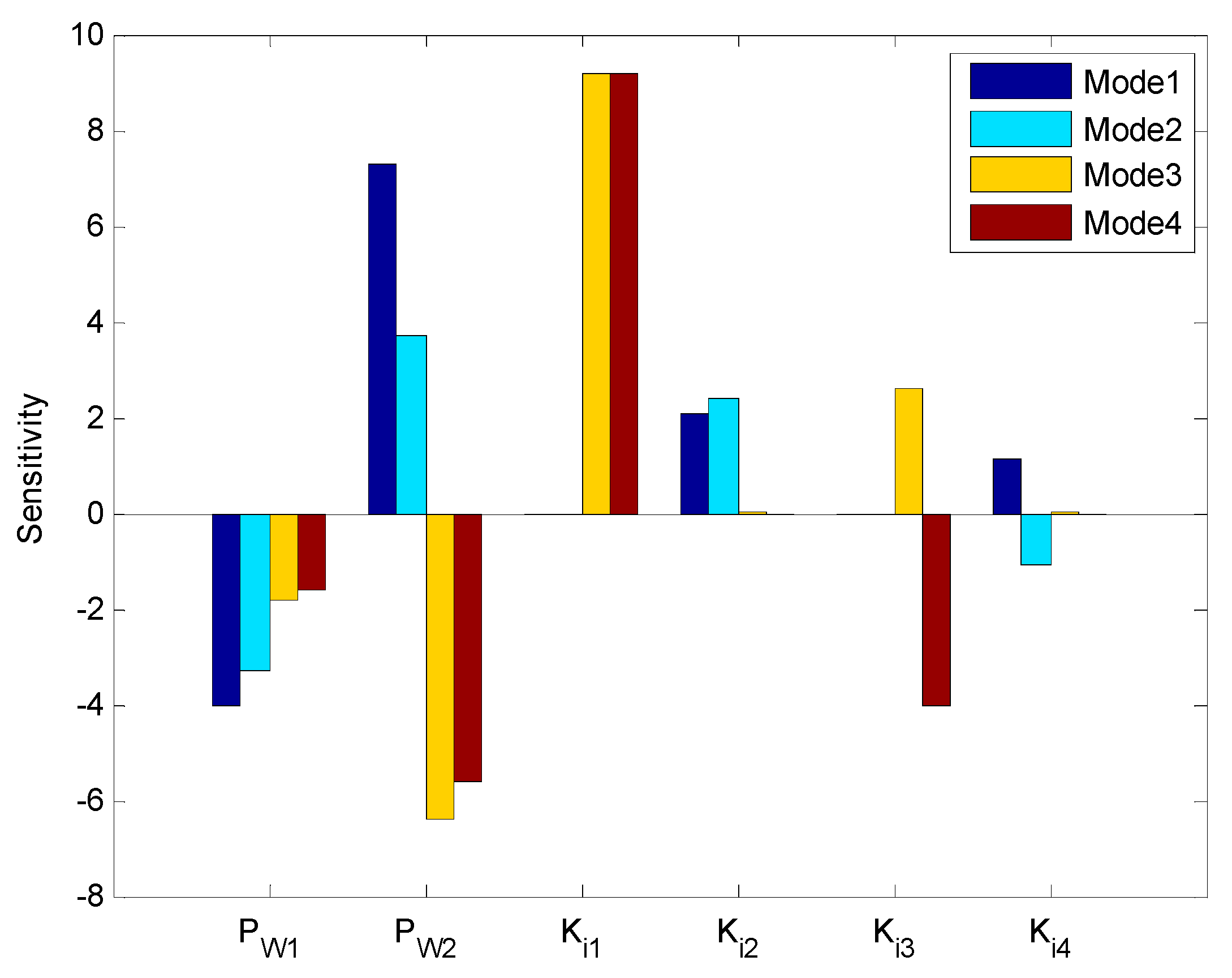
The effect of the output power of DFIGs on the oscillation propagation factor is analyzed below. When the DFIG1 output power reduces by 25%, the small-signal analysis result is shown in Table 2. The active power of DFIGs and the input vector are . The sensitivity with system subsynchronous oscillation frequency respect to DFIG active power and the PI controller parameters of DFIGs is shown in Figure 6. From Figure 6, it can be seen that the sensitivity of the oscillation propagation factor to the active power of DFIG2 is positive, indicating that as the active power of DFIG2 decreases, the oscillation propagation factor will decrease. The active power of DFIG2 is more sensitive to mode 4, which demonstrates that regulation of the active power of DFIG2 could block the oscillation propagation path.
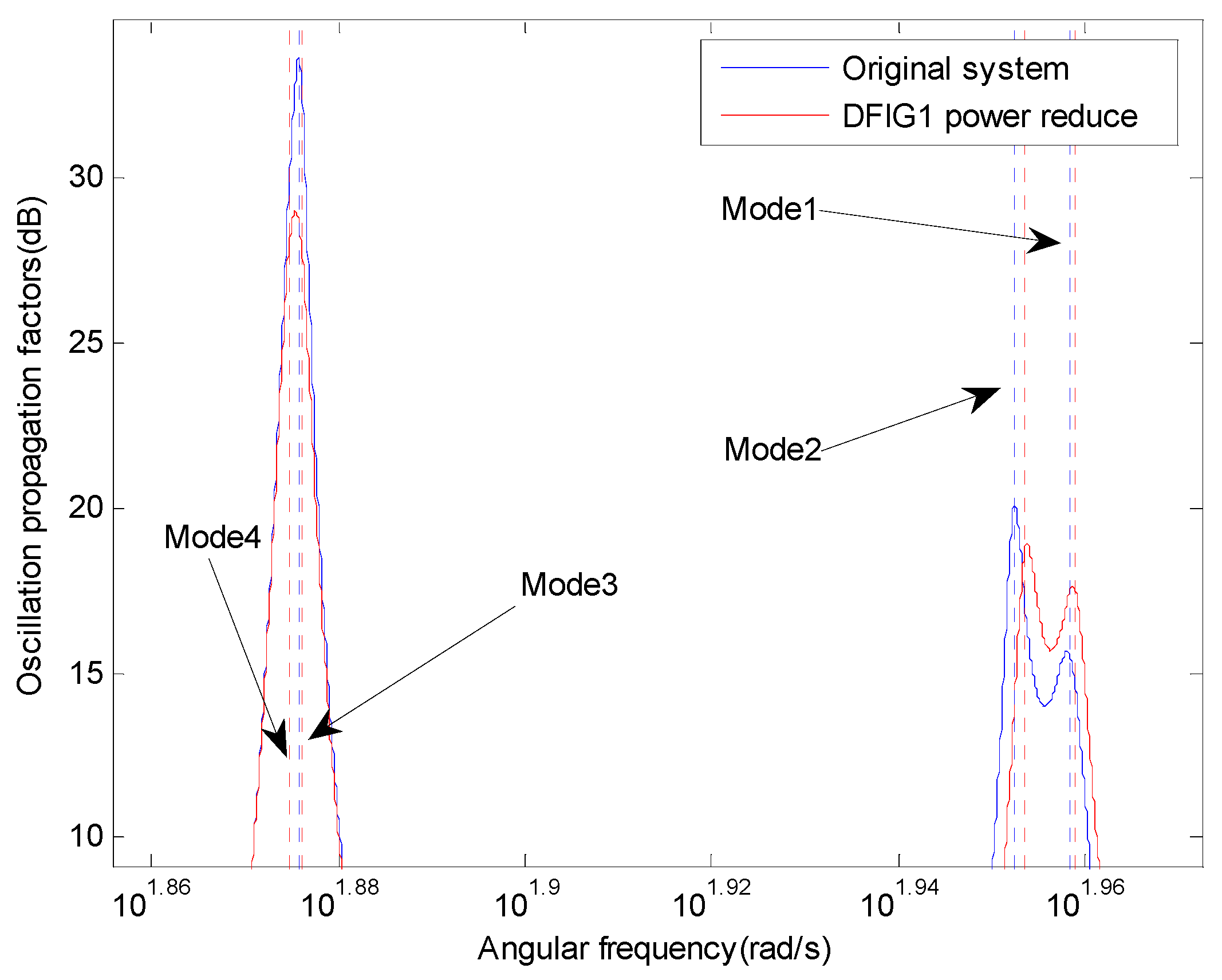
When the interharmonic currents from DFIG1 are injected to the power grid, the oscillation propagation factor of DFIG2 output power near the frequency of modes 1–4 is shown in Figure 7. The abscissa of the dotted line in Figure 7 is the system oscillation angular frequency. Comparing Table 1 and Table 2 after reducing the DFIG power, the damping ratio of system mode 1 decreases, and the damping ratios of system mode 2 and 3 increase. As can be seen from Figure 7, the oscillation propagation factor at the system angular frequency of mode 1 is increased. The oscillation propagation factor at the system angular frequency of mode 2 and 3 are decreased. The larger the system damping ratio, the smaller the oscillation propagation factor.
4.1.2. Time Domain Simulation Results
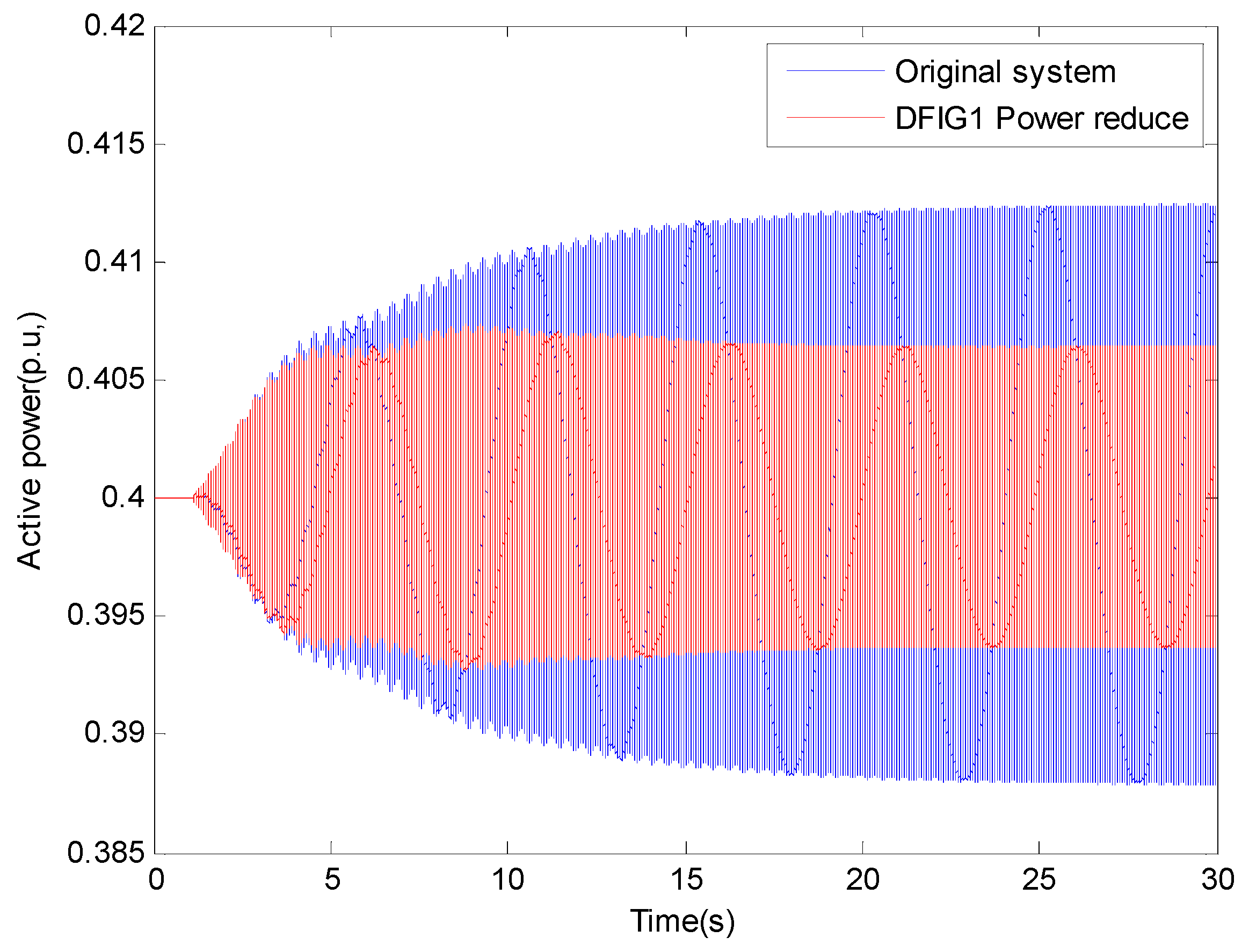
In order to verify the accuracy of the oscillation propagation factor analysis, the time domain simulations are carried out. The interharmonic currents from DFIG1 are injected at bus 6. The interharmonic current angular frequency is 89.64 rad/s, which is simulated under the condition that the original system and DFIG1 power are reduced respectively. The simulation results are shown in Figure 8.
When the amplitude of the active power oscillation is almost constant, the amplitude of the power oscillation can be obtained from the ordinate of the curve in the figure. The oscillation propagation factor can then be calculated based on (19), the definition of the oscillation propagation factor. In Figure 8, the interharmonic current at the original system bus 6 causes DFIG2 active power oscillation, the oscillation amplitude is 0.0124, and the oscillation propagation factor is 8.77, which is basically the same as the oscillation propagation factor at 89.61 rad/s in Figure 5. After the power of DFIG1 is reduced, the system damping increases, the oscillation propagation factor decreases, and the power oscillation amplitude decreases. The dynamic frequency domain analysis method based on transfer function can quantitatively describe the proportional relationship between the amplitude of power oscillation and the amplitude of interharmonic current.
4.2. New England 39 Bus System
The New-England 39 bus system [24] with two DFIGs is shown in Figure 9. The parameters of DFIGs in New-England 39 bus system are same as that in 4-machine 2-area system. The small-signal stability analysis was performed on the system shown in Figure 9, and the subsynchronous oscillation modes were obtained as shown in Table 3. The active power of DFIGs and the input vector are in Table 3.
4.2.1. Frequency Domain Simulation Results
The subsynchronous harmonics injected into the grid by DFIG1 are taken as input variables, and the active power of each generator is the output variable. The frequency response of each generator is as shown in Figure 10.
It can be seen from Figure 10 that when the interharmonic frequency is close to the oscillation frequency of the system, the oscillation propagation factors of each generator increase. Near the system subsynchronous frequency, the oscillation propagation factors of the two DFIG and part of the generator exceed 0 dB, and the output power is greatly affected by the subsynchronous oscillation caused by the interharmonics. When the input variable frequency is close to the frequencies of mode 3 and 4, the amplitude of the output power oscillation of the DFIG is larger than the amplitude of the synchronous generator output power oscillation. When the input variable frequency is close to the frequencies of mode 1 and 2, the amplitude of the output power oscillation of the DFIG is smaller than the amplitude of the synchronous generator output power oscillation. The oscillation propagation factor of DFIG2 is given in Figure 11.
The abscissa of the red dotted line in Figure 11 is the system oscillation angular frequency. In Figure 11, the two maximum value points of the DFIG2 oscillation propagation factor are 90.77 rad/s and 74.91 rad/s, respectively, which are close to the system oscillation angular frequency. When the interharmonic frequency is in the low frequency band, the power oscillation of DFIG2 is hardly caused. When the subsynchronous frequency interharmonics of the DFIG1 are injected into the power network, resonance is induced, and a large amplitude power oscillation of DFIG2 occurs.
The sensitivity with subsynchronous oscillation frequency respect to DFIG active power and the PI controller parameters of DFIGs are shown in Figure 12. Changes in controller parameters can cause changes in the propagation factor, and the amplitude of the oscillation of DFIGs changes. From Figure 12 it can be seen that is highly sensitive to the oscillation mode 3 and mode 4, which means the regulation of is effective for reducing the propagation aptitude. For the mode 1 and mode 2, is not sensitive, and the sensitivity is almost equal to zero, which means the regulation of could not help for reducing the propagation aptitude of mode 1 and mode 2. By this way, the parameters could be optimized to satisfy the engineering requirements.
4.2.2. Time Domain Simulation Results
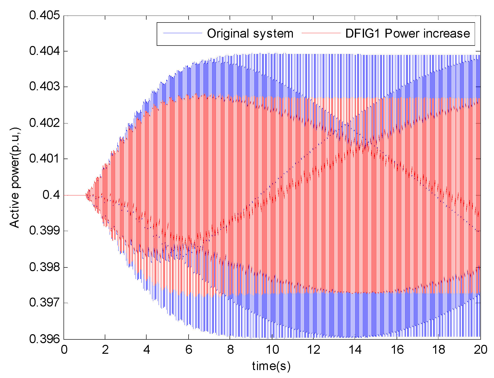
In the MATLAB, a time domain simulation model of New-England 39 bus System with two DFIGs is established, and an inter-harmonic current with an angular frequency of 90.77 rad/s and an amplitude of 0.001 is injected at bus 6. The DFIG2 active power simulation results are shown in Figure 13. The blue curve is the time domain simulation result of DFIG2 active power when the DFIG1 power is increased by a factor of 2. After the power of DFIG1 is increased, the system damping increases, the oscillation propagation factor decreases, and the power oscillation amplitude decreases. In Figure 13, the interharmonic current at bus 6 causes DFIG2 active power oscillation, the oscillation amplitude is 0.0039, and the oscillation propagation factor is 2.76, which is basically the same as the oscillation propagation factor at 90.77 rad/s in Figure 11.
5. Discussion
The evaluation of hazard degree of the subsynchronous oscillation needs to identify the propagation range of the subsynchronous oscillation. In order to maintain the stability of the power system, different methods are required according to different subsynchronous oscillation propagation ranges. The method for dealing with subsynchronous oscillation of power system is: When the oscillation propagation factor of the synchronous generator is larger than a given value, the subsynchronous oscillation propagation range includes the synchronous generators. The subsynchronous oscillation caused by the interharmonics is serious, and the DFIG that causes the subsynchronous harmonics needs to be shed [25]. When the synchronous generator is not included in the subsynchronous oscillation propagation range, the subsynchronous oscillation caused by the interharmonics is less harmful. It is not necessary to shed the DFIG that causes the subsynchronous harmonics. We can adjust the operating parameters of the DFIGs or take other measures.
Meanwhile, if a detailed electromagnetic transient model is established for a complete actual power system, it will take a lot of time to determine the subsynchronous oscillation propagation range by time domain simulation analysis. The method can quickly determine the subsynchronous oscillation propagation range by linearizing the transient model and using the oscillation propagation factor. When the DFIGs output is different, the oscillation propagation factor is different, then the oscillation amplitude at a different frequency is different. According to the participation factor [22], only the state variables with the highest participation in the oscillation mode can be obtained, but according to the oscillation propagation factor, the correlation degree between each generator and the oscillation with any frequency can be obtained. Through the sensitivity curve, it can be known that the change of the controller parameters will cause the change of the oscillation propagation factor, and the amplitude of the oscillation of DFIG2 will change.
6. Conclusions
The oscillation propagation factor which could characterize the subsynchronous oscillation magnitude propagation, is proposed in this paper. The interharmonics injected into the grid by DFIG will cause continuous oscillation of power. The oscillation propagation factor based on frequency domain method is used to study the propagation characteristics of DFIG interharmonic injected into the grid. The main conclusions are as follows: The oscillation propagation factor can quantify the strength of the subsynchronous oscillation, and could give the propagation intensity to different directions or different devices. The oscillation propagation factor generally has a maximum point at the oscillation frequency of the system, and the amplitude of the power oscillation increases significantly. The sensitivities of the operating parameters and system parameters to the oscillation propagation factor are deduced to give the guidance for blocking the oscillation propagation path.
Author Contributions
Conceptualization, J.D. and T.W.; Methodology, J.Y.; Software, J.Y.; Validation, Z.W., and S.P.; Formal Analysis, J.D.; Investigation, J.D.; Resources, S.P.; Writing-Original Draft Preparation, T.W.; Writing-Review & Editing, J.Y.; Visualization, H.H.; Supervision, F.C.; Project Administration, T.W.; Funding Acquisition, T.W.
Funding
This research was funded by Fundamental Research Funds for the Central Universities grant number 2018MS006.
Conflicts of Interest
The authors declare no conflict of interest.
References
- Leon, A.E. Integration of DFIG-Based Wind Farms Into Series-Compensated Transmission Systems. IEEE Trans. Sustain. Energy 2017, 7, 451–460. [Google Scholar] [CrossRef]
- Liu, H.; Xie, X.; Zhang, C.; Li, Y.; Liu, H.; Hu, Y. Quantitative SSR analysis of series-compensated DFIG-based wind farms using aggregated RLC circuit model. IEEE Trans. Power Syst. 2017, 32, 474–483. [Google Scholar] [CrossRef]
- Gao, F.; He, Q.; Hao, Z.; Zhang, B. The research of subsynchronous oscillation in PMSG wind farm. In Proceedings of the IEEE PES AsiaPacificPower and Energy Engineering Conference (APPEEC), Xi’an, China, 25–28 October 2016; pp. 1883–1887. [Google Scholar]
- Dincer, I. Renewable energy and sustainable development: A crucial review. Renew. Sustain. Energy Rev. 2000, 4, 157–175. [Google Scholar] [CrossRef]
- Khan, M.A.A.; Shahriar, M.M.; Islam, M.S. Power quality improvement of DFIG and PMSG based hybrid wind farm using SMES. In Proceedings of the International Conference on Electrical & Electronic Engineering (ICEEE), Ankara, Turkey, 8–10 April 2017; pp. 1–4. [Google Scholar]
- Fan, L.; Yuvarajan, S.; Kavasseri, R. Harmonics analysis of a DFIG for a wind energy conversion system. IEEE Trans. Energy Convers. 2010, 25, 181–190. [Google Scholar] [CrossRef]
- Djurović, S.; Vilchis-Rodriguez, D.S.; Smith, A.C. Supply induced interharmonic effects in wound rotor and doubly-fed induction generators. IEEE Trans. Energy Convers. 2015, 30, 1397–1408. [Google Scholar] [CrossRef]
- Wen, T.; Huang, Y.; Zhao, D.; Zhu, L.; Wang, X. Mechanism of Sub-synchronous Interaction caused by inter-harmonics in DFIG. J. Eng. 2017, 13, 892–896. [Google Scholar] [CrossRef]
- Dong, X.; Zang, W.; Dong, C.; Xu, T. SSR characteristics study considering DFIGs at different locations in large wind farm. In Proceedings of the China International Conference on Electricity Distribution (CICED), Xi’an, China, 10–13 August 2016; pp. 1–6. [Google Scholar]
- Leon, A.E.; Solsona, J.A. Sub-synchronous interaction damping control for DFIG wind turbines. IEEE Trans. Power Syst. 2015, 30, 419–428. [Google Scholar] [CrossRef]
- Cheng, Y.; Sahni, M.; Muthumuni, D.; Badrzadeh, B. Reactance scan crossover-based approach for investigating SSCI concerns for DFIG-based wind turbines. IEEE Trans. Power Deliv. 2013, 28, 742–751. [Google Scholar] [CrossRef]
- Suriyaarachchi, D.H.R.; Annakkage, U.D.; Karawita, C.; Jacobson, D.A. A Procedure to Study Sub-Synchronous Interactions in Wind Integrated Power Systems. IEEE Trans. Power Syst. 2013, 28, 377–384. [Google Scholar] [CrossRef]
- Fan, L.; Miao, Z. Nyquist-stability-criterion-based SSR explanation for type-3 wind generators. IEEE Trans. Energy Conv. 2012, 27, 807–809. [Google Scholar] [CrossRef]
- Sun, J. Impedance-based stability criterion for grid-connected inverters. IEEE Trans. Power Electron. 2011, 26, 3075–3078. [Google Scholar] [CrossRef]
- Cespedes, M.; Sun, J. Modeling and mitigation of harmonic resonance between wind turbines and the grid. In Proceedings of the IEEE Energy Conversion Congress and Exposition, Phoenix, AZ, USA, 17–22 September 2011; pp. 2109–2116. [Google Scholar]
- Wu, F.; Zhang, X.; Godfrey, K.; Ju, P. Modeling and Control of Wind Turbine with Doubly Fed Induction Generator. In Proceedings of the IEEE PES Power Systems Conference and Exposition, Atlanta, GA, USA, 29–31 October 2006; pp. 1404–1409. [Google Scholar]
- Qiao, W. Dynamic modeling and control of doubly fed induction generators driven by wind turbines. In Proceedings of the IEEE PES Power Systems Conference and Exposition, Seattle, WA, USA, 15–18 March 2009; pp. 1–8. [Google Scholar]
- Erdogan, N.; Henao, H.; Grisel, R. A proposed Technique for Simulating the Complete Electric Drive Systems with a Complex Kinematics Chain. In Proceedings of the 2007 IEEE International Electric Machines & Drives Conference, Antalya, Turkey, 3–5 May 2007; pp. 1240–1245. [Google Scholar]
- Abad, G.; Rodriguez, M.A.; Iwanski, G.; Poza, J. Direct Power Control of Doubly Fed Induction Generator based Wind Turbines under Unbalanced Grid Voltage. IEEE Trans. Power Electron. 2010, 25, 442–452. [Google Scholar] [CrossRef]
- Jiang, J.; Chao, Q.; Chen, J.; Chang, X. Simulation study on frequency response characteristic of different wind turbines. Renew. Energy Resour. 2010, 28, 24–28. [Google Scholar]
- Skogestad, S.; Postlethwaite, I. Multivariable Feedback Control: Analysis and Design; John Wiley & Sons: Hoboken, NJ, USA, 2005. [Google Scholar]
- Kundur, P. Power System Stability and Control; Balu, N.J., Lauby, M.G., Eds.; McGraw-Hill: New York, NY, USA, 1994; Volume 7. [Google Scholar]
- Holmes, D. Pulse Width Modulation for Power Converters: Principles and Practice; JohnWiley & Sons: Hoboken, NJ, USA, 2003. [Google Scholar]
- Pai, M.A. Energy Function Analysis for Power System Stability; Kluwer Academic Publishers: Boston, MA, USA, 1989. [Google Scholar]
- Xie, X.; Liu, W.; Liu, H.; Du, Y.; Li, Y. A system-wide protection against unstable SSCI in series-compensated wind power systems. IEEE Trans. Power Deliv. 2018, 33, 3095–3104. [Google Scholar] [CrossRef]
Figure 1.
Doubly fed induction generator (DFIG) based wind energy system.

Figure 2.
4-machine 2-area test system with two DFIGs.
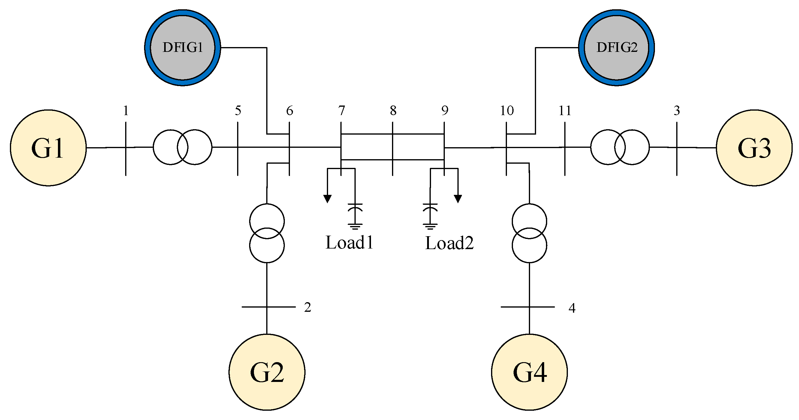
Figure 3.
Oscillation propagation factor of each generator.

Figure 4.
Oscillation propagation factor near the oscillation frequency.

Figure 5.
Oscillation propagation factor of DFIG2.

Figure 6.
The sensitivity of DFIG2 oscillation propagation factor.
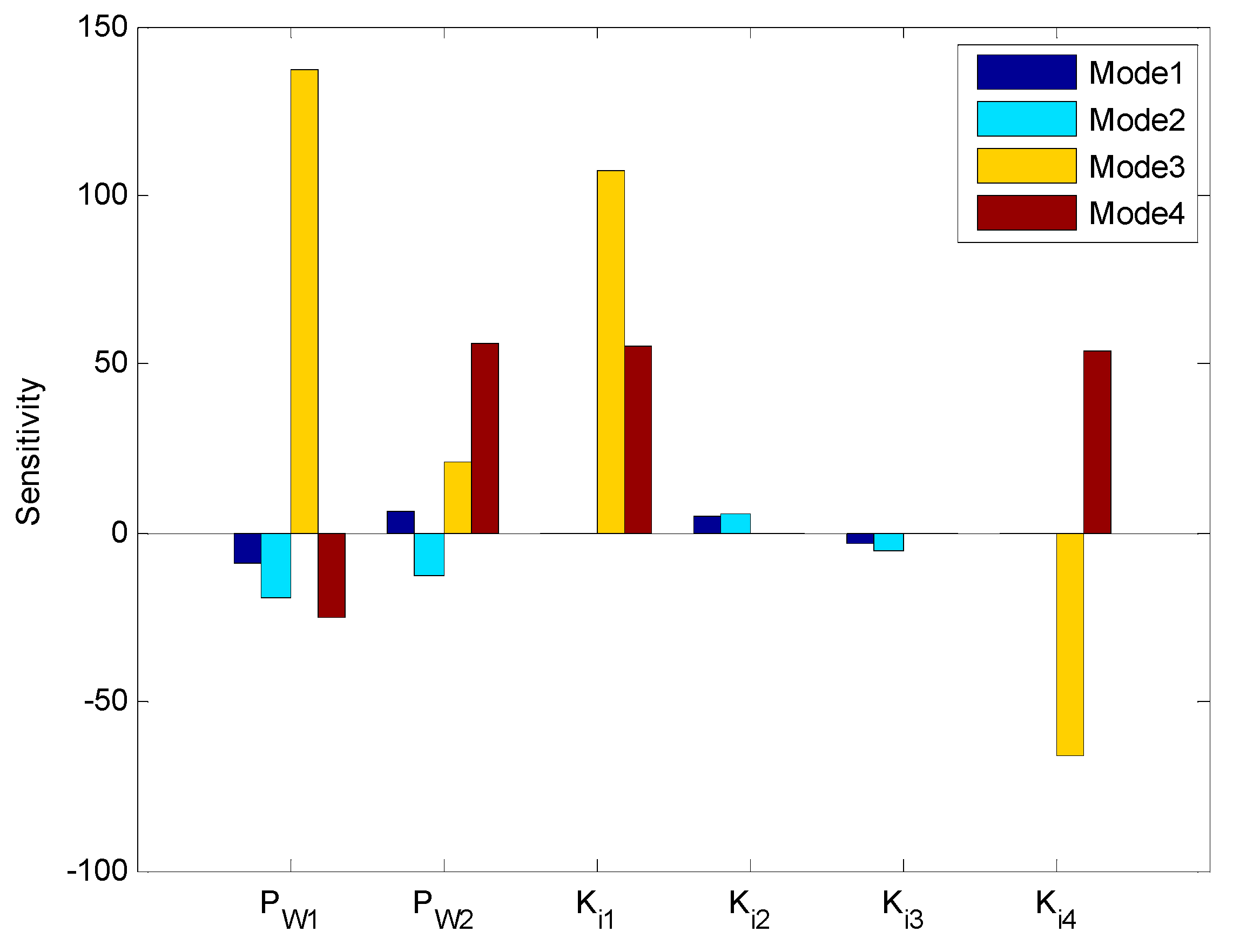
Figure 7.
The oscillation propagation factors curve of DFIG2.

Figure 8.
The output active power of DFIG2.

Figure 9.
The New-England 39 bus system with two DFIGs.
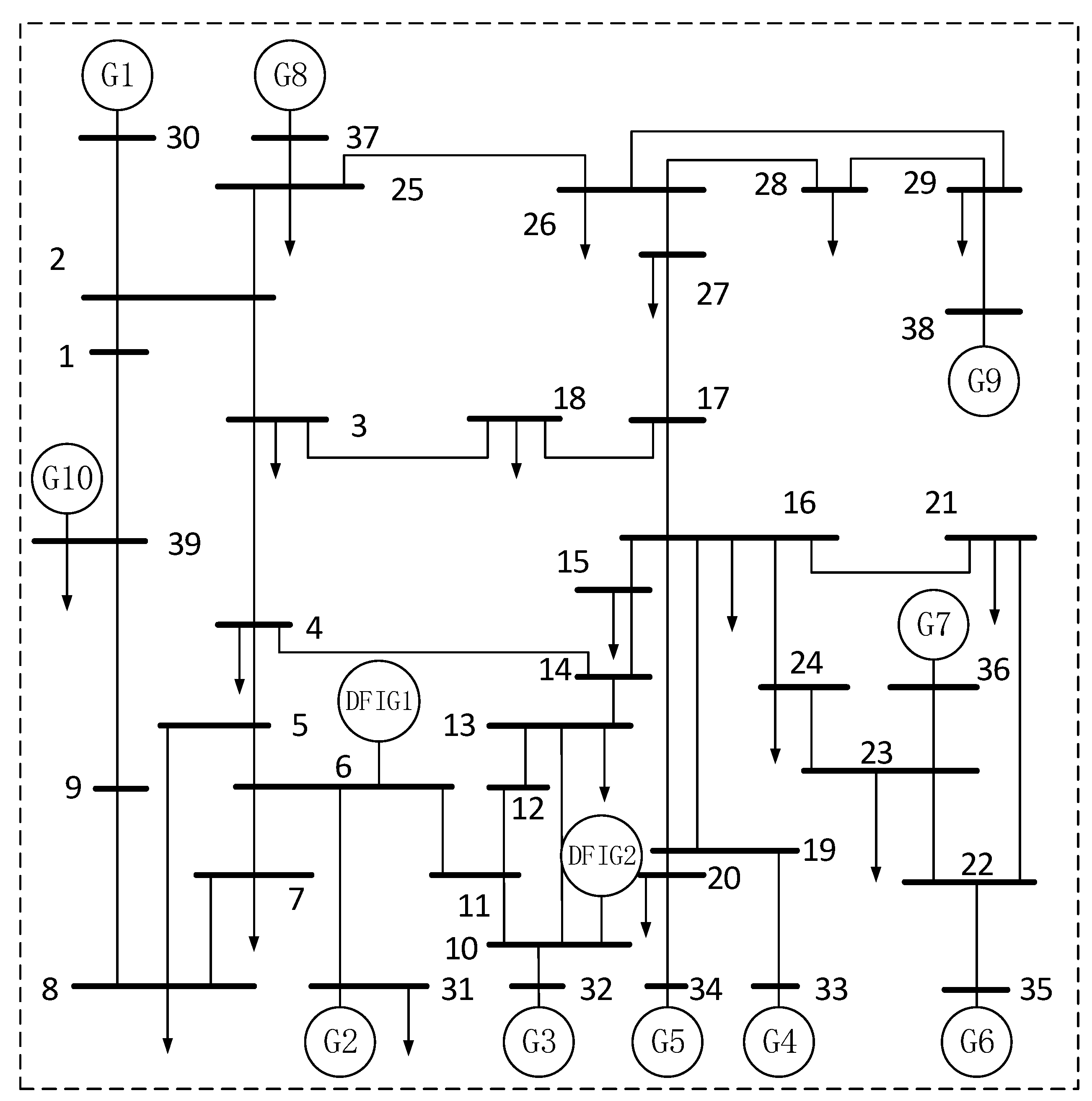
Figure 10.
Oscillation propagation factor of each generator.
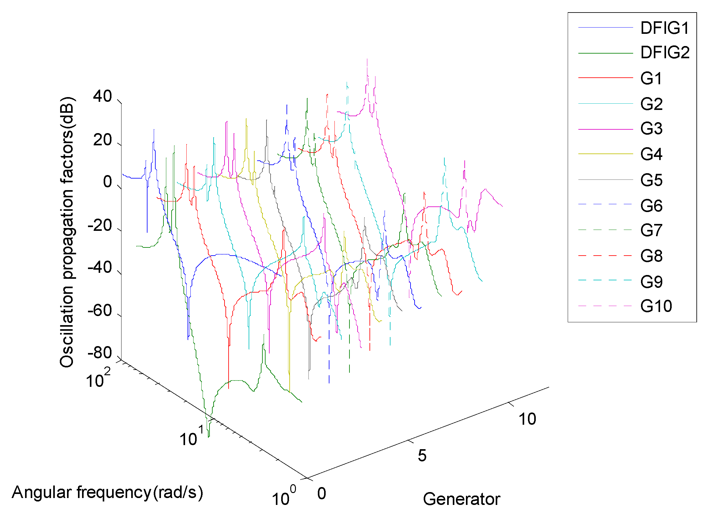
Figure 11.
Oscillation propagation factor of DFIG2.
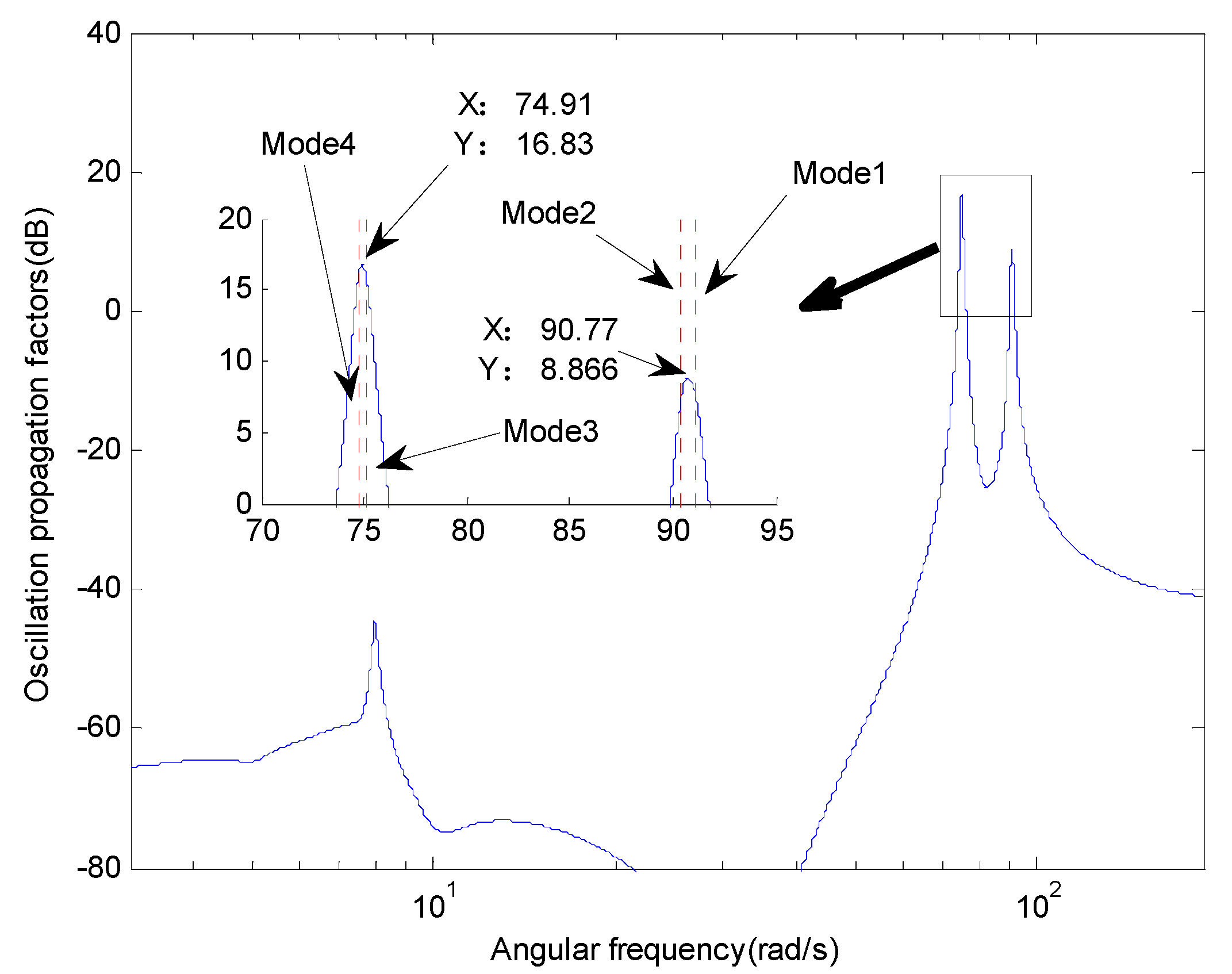
Figure 12.
The sensitivity of DFIG2 oscillation propagation factor.

Figure 13.
The output active power of DFIG2.


Table 1.
System oscillation modes.
| Mode | Eigenvalue | Angular Frequency (Rad/s) | Damping Ratio |
|---|---|---|---|
| 1 | −0.3364 ± 90.8578j | 90.8578 | 0.0037 |
| 2 | −0.1806 ± 89.5917j | 89.5917 | 0.0020 |
| 3 | −0.1297 ± 75.1461j | 75.1461 | 0.0017 |
| 4 | −0.2758 ± 74.9510j | 74.9510 | 0.0037 |
| 5 | −0.0368 ± 13.3422j | 13.3422 | 0.0028 |
| 6 | −0.0403 ± 12.4648j | 12.4648 | 0.0032 |
| 7 | −0.0355 ± 6.5300j | 6.5300 | 0.0054 |
Table 2.
System oscillation mode.
| Mode | Eigenvalue | Angular Frequency (Rad/s) | Damping Ratio |
|---|---|---|---|
| 1 | −0.2973 ± 90.9755j | 90.9755 | 0.0033 |
| 2 | −0.2285 ± 89.8449j | 89.8449 | 0.0025 |
| 3 | −0.2367 ± 75.1553j | 75.1553 | 0.0031 |
| 4 | −0.2539 ± 74.9392j | 74.9392 | 0.0034 |
| 5 | −0.0373 ± 13.3797j | 13.3797 | 0.0028 |
| 6 | −0.0403 ± 12.4733j | 12.4733 | 0.0032 |
| 7 | −0.0395 ± 6.3194j | 6.3194 | 0.0062 |
Table 3.
System subsynchronous oscillation mode.
| Mode | Eigenvalue | Angular Frequency (Rad/s) | Damping Ratio |
|---|---|---|---|
| 1 | −0.5060 ± 90.4108j | 90.4108 | 0.0056 |
| 2 | −0.5494 ± 91.0655j | 91.0655 | 0.0060 |
| 3 | −0.4586 ± 74.7992j | 74.7992 | 0.0061 |
| 4 | −0.5610 ± 75.0893j | 75.0893 | 0.0075 |
© 2019 by the authors. Licensee MDPI, Basel, Switzerland. This article is an open access article distributed under the terms and conditions of the Creative Commons Attribution (CC BY) license (http://creativecommons.org/licenses/by/4.0/).
Share and Cite
MDPI and ACS Style
Wen, Z.; Peng, S.; Yang, J.; Deng, J.; He, H.; Wang, T. Analysis of the Propagation Characteristic of Subsynchronous Oscillation in Wind Integrated Power System. Energies 2019, 12, 1081. https://doi.org/10.3390/en12061081
AMA Style
Wen Z, Peng S, Yang J, Deng J, He H, Wang T. Analysis of the Propagation Characteristic of Subsynchronous Oscillation in Wind Integrated Power System. Energies. 2019; 12(6):1081. https://doi.org/10.3390/en12061081
Chicago/Turabian StyleWen, Zhiping, Shutao Peng, Jing Yang, Jun Deng, Hanqing He, and Tong Wang. 2019. "Analysis of the Propagation Characteristic of Subsynchronous Oscillation in Wind Integrated Power System" Energies 12, no. 6: 1081. https://doi.org/10.3390/en12061081
Note that from the first issue of 2016, this journal uses article numbers instead of page numbers. See further details here.