Embedded Discrete Fracture Modeling as a Method to Upscale Permeability for Fractured Reservoirs

Abstract

Fractured reservoirs are distributed widely over the world, and describing fluid flow in fractures is an important and challenging topic in research. Discrete fracture modeling (DFM) and equivalent continuum modeling are two principal methods used to model fluid flow through fractured rocks. In this paper, a novel method, embedded discrete fracture modeling (EDFM), is developed to compute equivalent permeability in fractured reservoirs. This paper begins with an introduction on EDFM. Then, the paper describes an upscaling procedure to calculate equivalent permeability. Following this, the paper carries out a series of simulations to compare the computation cost between DFM and EDFM. In addition, the method is verified by embedded discrete fracture modeling and fine grid methods, and grid-block and multiphase flow are studied to prove the feasibility of the method. Finally, the upscaling procedure is applied to a three-dimensional case in order to study performance for a gas injection problem. This study is the first to use embedded discrete fracture modeling to compute equivalent permeability for fractured reservoirs. This paper also provides a detailed comparison and discussion on embedded discrete fracture modeling and discrete fracture modeling in the context of equivalent permeability computation with a single-phase model. Most importantly, this study addresses whether this novel method can be used in multiphase flow in a reservoir with fractures.

1. Introduction

Fractures, whether naturally occurring or hydraulically created, occur at different length scales with different densities in geological porous media. Fractures have a great impact on the quality of a porous medium. Understanding fractures is important for describing the challenges inherent to hydrocarbon flow in porous media. Two main methods are used to model fluid flow through fractured rocks. One is discrete fracture modeling (DFM), and the other is equivalent continuum modeling.

DFM explicitly describes matrix and fracture systems [1], can be used for modeling fractured reservoirs when the properties of the porous media are heterogeneous [2], and is considered one of the most accurate methods to describe fluid flow through a fracture and matrix system. However, a main drawback of this method is that meshing a complex three-dimensional (3D) fracture network is very difficult. Another drawback is the high computational cost due to a large number of grids and convergence problems. Given the improvement of computational efficiency, though, DFM is becoming more and more attractive; however, its application at the field scale is not realistic at present [3,4]. Accurately describing fluid flow in porous media with fractures can be achieved by DFM, but the meshing of complex fracture networks and the increase in grid number limit the application of this method for field-scale simulation.

Embedded discrete fracture modeling (EDFM), as a special form of DFM introduced by Li and Lee [5], uses a structured grid to represent the matrix and introduces additional fracture control volumes by computing the intersection of fractures with the matrix grid. Compared to DFM, this method avoids the requirement for a conforming mesh and allows for conventional corner-point grids. Recently, more attention has been paid to EDFM because of its flexibility and accuracy. The iterative multiscale finite volume (i-MSFV) approach was introduced by Hadi Hajibeygi [6] to improve efficiency and accuracy for fractured porous media, and the results are very promising. Tene et al. [7,8] proposed projection-based EDFM to deal with cases where fracture permeability lies below that of the matrix. Li et al. [9] introduced a technique integrating EDFM and the dual-porosity-dual-permeability (DPDP) method to simulate fluid flow in fractured reservoirs.

The equivalent continuum model was proposed by Barrenblatt [10] and then was improved by Warren and Root [11] and Pruess [12]. In equivalent continuum models, the hydraulic properties (permeability and porosity) of fractures are combined to create matrix-grid blocks. Due to computational efficiency, equivalent continuum models (single, dual, or multiple models), especially the dual-porosity model, have been used widely in the oil and gas industry for modeling fluid flow in fractured rocks. Accurate calculation of equivalent permeability (termed permeability upscaling) is the key to applying this method.

Snow [13] studied the permeability of fractured porous rock, and Oda [14] proposed an analytical method to compute equivalent permeability based on geometric characteristics of fractures. Oda’s method is employed widely for reservoir simulation, even though it is less accurate for calculating fracture connectivity, as pointed out by Elfeel and Geiger [15].

Flow-based upscaling is another approach for computing equivalent permeability based on solving the flow problem with the DFM method. Based on the flow rate and pressure gradient computation approach, Durlofsky [16,17] classified flow-based upscaling methods into two groups: the boundary integration method and the volume averaging method. Long et al. [18] used the finite element method to resolve the flow problem within fractures and to calculate equivalent permeability with a linear boundary. Koudina et al. [19] introduced the finite volume method with unstructured grids to study equivalent permeability. However, the method does not take fluid flow in the matrix into consideration, which limits its application (Kaufmann et al. [20]). Recently, Lough et al. [21] used the boundary element method, and Bogdanov et al. [22] extended Koudina et al.’s [19] method, to calculate equivalent permeability. Both methods took into consideration matrix permeability. More recently, a volume-averaging method based on the finite element method was proposed by Lang et al. [23] to find equivalent permeability in fractured porous media. Fumagalli et al. [4,24] used EDFM to calculate fracture–fracture and matrix–fracture transmissibilities, with a remarkable gain in speedup.

The aim of this research was to enable the modeling of flow in the upscaling grid by computing equivalent permeability for matrix blocks with fractures. In this work, we have developed a new flow-based upscaling approach to calculate equivalent permeability based on solving the flow problem with the EDFM method for fractured rocks. We have validated this method on simple and complex fracture networks. Our original contribution is the employment of EDFM to compute equivalent permeability for a fractured reservoir. Another application of our approach is the possibility to deal with all kinds of fractures, such as vertical and inclined complex cracks, which prove difficult for permeability upscaling using the DFM method.

This paper begins with an introduction to the EDFM method in Section 2. A permeability upscaling procedure based on EDFM for fractured reservoirs is described in Section 3. Section 4 presents several numerical examples to evaluate the performance and validity of the method. In particular, we compare performance among the DFM method (fine grid model), the EDFM method, and the proposed upscaling approach for a sample of fractures. Then, we validate the new method for single-phase and multiphase flow and study the performance for different grid-block numbers in the upscaling process. We address comparisons between the proposed upscaling approach and the EDFM method used in the oil industry for a realistic 3D case. Section 5 gathers conclusions and presents an outlook on flow-based upscaling for fractured reservoirs.

2. Embedded Discrete Fracture Modeling

EDFM was introduced by Li and Lee [5] and was expanded on by Moinfar et al. [25] and Tene et al. [26]. Unlike DFM, the EDFM method does not require generating complex meshing and can use conventional corner-point grids, which alleviate the computational cost for complex fracture modeling.

In this method, we need to define the corner-point cell for the matrix and then embed fractures into the matrix cells (Figure 1); after that, we define intersection faces between different media, for example, matrix and fracture. Once we have defined all cells and have found the intersections between them, we can proceed to compute transmissibility, which is a key aspect of EDFM. Figure 2 illustrates the connection list of continua in the computational domain for a simple scenario. As mentioned by Li et al. [9], there are four types of connection:

• Type one: Conductivity between matrix grids
• Type two: Conductivity between fracture segments inside an individual fracture
• Type three: Conductivity between intersecting fracture segments
• Type four: Conductivity between fracture and matrix

Figure 2a shows four matrix cells and two fractures, with fracture one divided into segments F1 and F2 by matrix cells and fracture two divided into segments F3 and F4 by matrix cells. Figure 2b shows the connections among different media. Black lines indicate the connection between matrix cells; green lines indicate the connection between matrix and fracture; red lines show the connection between fracture segments in an individual fracture; and the blue line is the connection of intersecting fractures.

2.1. Type One: Conductivity between Matrix Grids

The transmissibility factor between matrix cells (the black lines indicated in Figure 2b) in the model depends on the matrix permeability and matrix geometry, which was given by Li et al. [9]. Equation (1) refers to the transmissibility factor between matrix cells:

$$T_{mij}=\frac{k_{mij}{A}_{mij}}{d_{mij}}$$

(1)

where

$A_{mij}$ is the contact area between matrix cells i and j.

$k_{mij}$ is the average permeability tensor for matrix cells i and j, which can be defined as follows:

$$k_{mij}=\frac{2\ast k_{m_i}{k}_{m_j}}{k_{m_i}+k_{m_j}}$$

(2)

where

$k_{mi}$, $k_{mj}$ are the permeability tensors for matrix cells i and j, respectively.

$d_{mij}$ is the average normal distance between matrix cells i and j.

2.2. Type Two: Conductivity between Fracture Segments Inside an Individual Fracture

Karimi-Fard et al. [3] introduced a two-point flux approximation scheme to calculate the transmissibility factor between fracture segments in an individual fracture (F1 and F2, F3 and F4 in Figure 2b). The transmissibility factor was defined as follows:

$$T_{fifj}=\frac{2\ast T_{fi}{T}_{fj}}{T_{fi}+T_{fj}}$$

(3)

$$T_{fi}=\frac{k_{fi}{A}_c}{d_{segi}}$$

(4)

$$T_{fj}=\frac{k_{fj}{A}_c}{d_{segj}}$$

(5)

where

$k_{fi},k_{fj}$ are the permeability tensors for fracture segments i and j, respectively.

$A_c$ is the contact area for two segments.

$d_{segi}$, $d_{segj}$ are the distances from the centroids of fracture segments i and j to the contact face, respectively.

2.3. Type Three: Conductivity between Intersecting Fracture Segments

The calculation method for transmissibility between intersecting fracture segments (the blue lines indicated in Figure 2b) was given by Moinfar et al. [25] and is defined as follows:

$$T_{int}=\frac{2\ast T_i{T}_j}{T_i+T_j}$$

(6)

$$T_i=\frac{k_{fj}{w}_{fj}{L}_{int}}{d_{fi}}$$

(7)

$$T_j=\frac{k_{fj}{w}_{fj}{L}_{int}}{d_{fj}}$$

(8)

where

$L_{int}$ is the length of the intersection line.

$k_{fi},k_{fj}$ are the permeabilities of fractures i and j, respectively.

$w_{fi},w_{fj}$ are the apertures of fractures i and j, respectively.

$d_{fi}$, $d_{fj}$ are the distances from the centroids of the segments i and j to the intersection line, respectively.

2.4. Type Four: Conductivity between Fracture and Matrix

The transmissibility factor between the matrix and fracture segment (the green lines indicated in Figure 2b) depends on the matrix permeability and fracture geometry, which was given by Li et al. [9]. When a fracture segment fully penetrates a matrix cell, the matrix–fracture transmissibility factor is as follows:

$$T_{f-m}=\frac{k_{mf}{A}_{mf}}{d_{f-m}}$$

(9)

where

$A_{mf}$ is the area of the fracture segment on one side.

$k_{mf}$ is the permeability tensor, which is calculated as follows:

$$k_{mf}=\frac{2\ast k_f{k}_m}{k_f+k_m}$$

(10)

where

$k_f$ is the permeability tensor for the fracture.

$k_m$ is the permeability tensor for the matrix.

$d_{f-m}$ is the average normal distance from the matrix to the fracture.

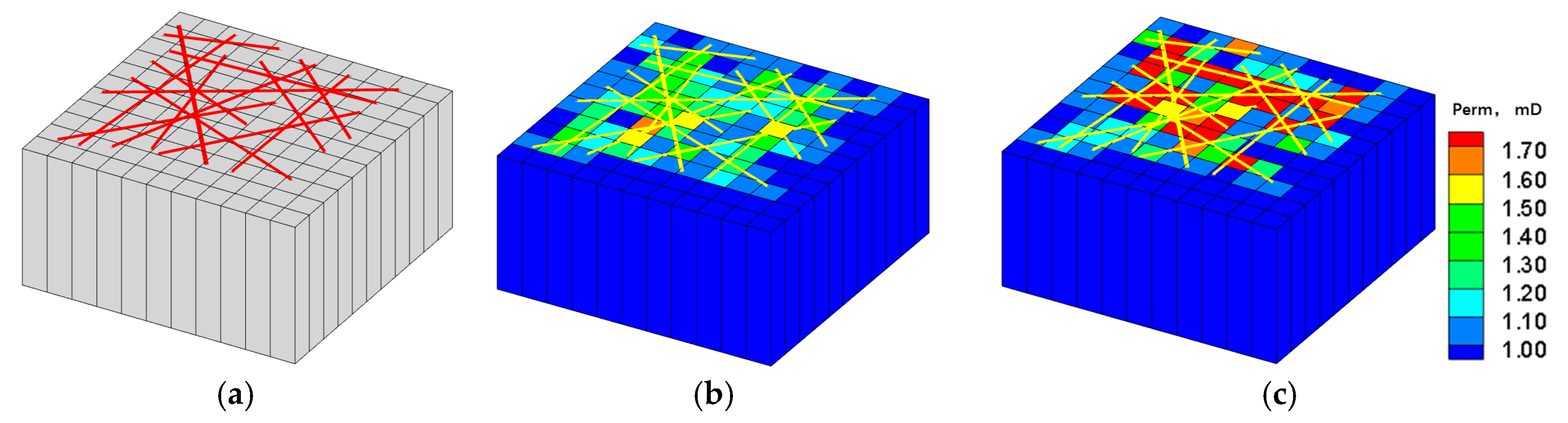
3. Upscaling Procedure

As pointed out by Fumagalli [4,24], along with the increase in the number of fractures, the degree of difficulty in generating fracture grids using EDFM/DFM is rising, and the number of grids is increasing, both leading to an increase in computation cost, which limits the application of EDFM/DFM for complex fracture systems. Therefore, different strategies are required to solve this problem, such as equivalent continuum modeling. In equivalent continuum modeling, an upscaling process is needed. Durlofsky [16] gave a comprehensive review of upscaling techniques in porous media without fractures. In this study, our main goal is to upscale grid properties (focusing on permeability) for fractured reservoirs. This section shows the procedure for upscaling based on EDFM. The entire procedure presented in this section is summarized as Figure 3.

During the upscaling process, we first receive the matrix grid-block and its properties from commercial software, such as Petrel [27] or CMG [28]. The information usually includes eight-point positions of each grid-block in a corner-point grid system, as well as its porosity, permeability, and saturation. We also obtain fracture information, such as fracture distribution, permeability, and porosity, from commercial software, such as Fracman [29] or the fracture module in Petrel. Using the information gained from the above two steps, we can generate a matrix grid and fracture distribution for a two-dimensional (2D) case (Figure 4).

Next, for all cells, we apply the following process:

Choose a cell, keep the matrix and fracture geometry and property information, and divide the cell into NX × NY × NZ, which may change for different cases and should be optimized sometimes (as shown in Figure 4a,b).

Define the flow boundary for the new grid system. In this study, we use a constant pressure boundary in the flow direction and a closed boundary for the other two sides, as shown in Figure 5.

Step 1:

Initialize the new grid system. Assign properties values for the matrix and fractures, such as porosity, permeability, and saturation, which are inherited from the original big model. We also need to define the connection and calculate the transmissibility among different media using Equations (1)–(10). Figure 6 shows an example of connection. We also define the well and production in this step.

Step 2:

We calculate the flow rate and apply the Darcy flow equation to calculate the whole grid system’s permeability, which combines the matrix and fracture flow capacity.

4. Numerical Examples

To evaluate and validate the performance of the new method introduced in Section 3, a series of simulation cases are presented in this section. In Section 4.1, we validate the EDFM by comparison with the DFM model. In Section 4.2, we compare the computation time and performance among the DFN method, the EDFM method, and the proposed upscaling approach for a sample of fractures. Then, in Section 4.3, we validate the new upscaling approach. A series of simulation cases is studied for the grid block and multiphase in Section 4.4. In Section 4.5, we compare the proposed approach and the EDFM method for a 3D case with complex fractures.

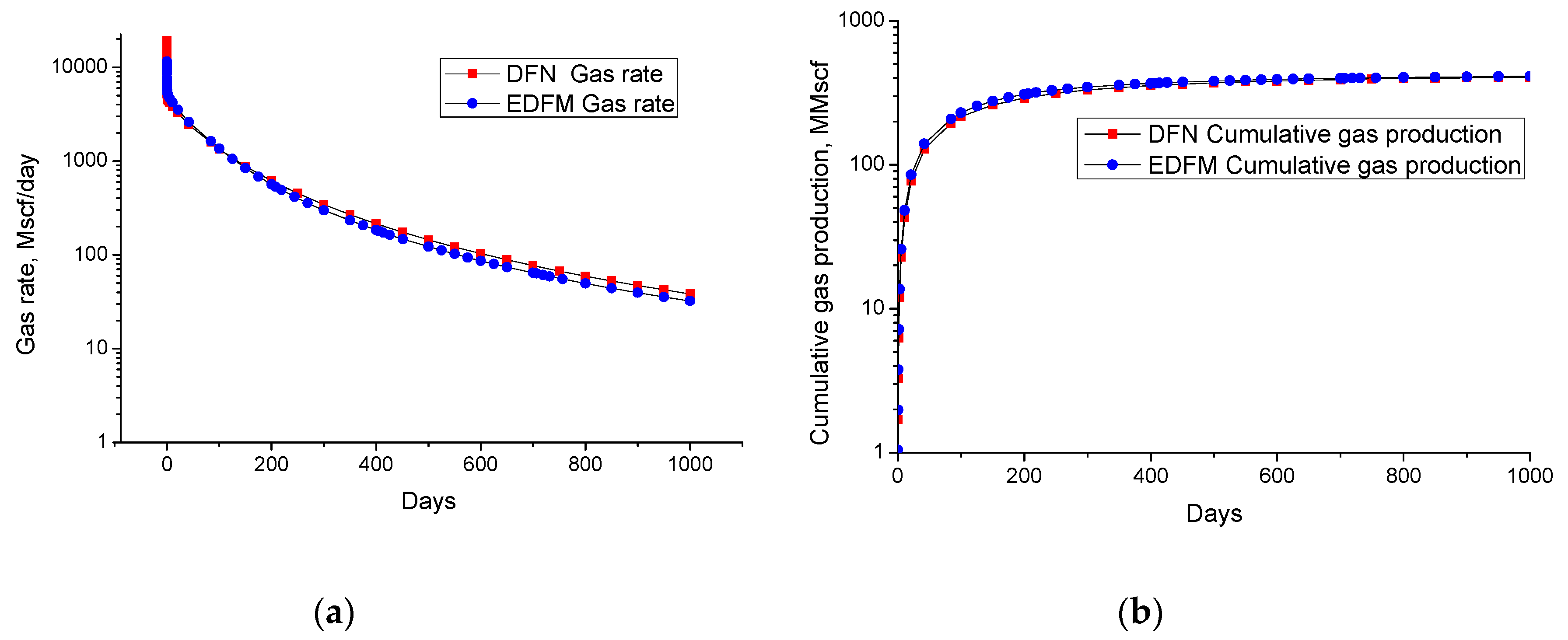
4.1. Validating the EDFM Method

As mentioned in the introduction section, DFM is the classic method used for upscaling fracture permeability. In this section, computation time and gas rate for EDFM and DFM are compared by testing a model with 251 fractures (Figure 7a). The matrix grid number is 5000 (50 × 50 × 2) in the EDFM model (Figure 7b), while the DFM model includes 238,762 cells (Figure 7c). In the model, matrix permeability is set to 1 mD, and fracture permeability is 5000 mD. A gas well in the center of the model with a constant rate is assumed in the study. Figure 8 presents that the two methods obtain the same gas rate. The computation time for the DFM is 287 seconds and for the EDFM is 73 seconds based on the same computation environment for single-phase flow. These results indicate that EDFM performs better than the DFM method, as one of EDFM’s main advantages is that it avoids the need to generate complex grids for fractures and the matrix.

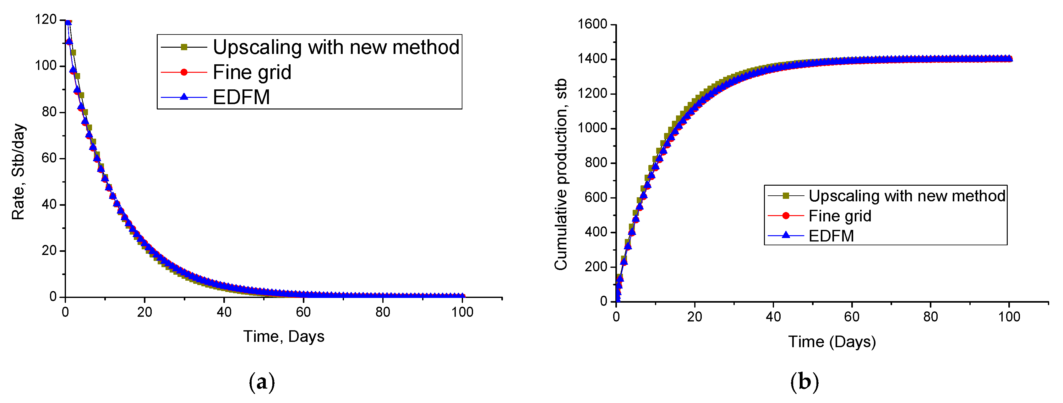
4.2. Validating the New Upscaling Approach by Comparison with the DFM Method

As shown in Figure 9, a cell model with two fractures is used to compare the EDFM and DFN model for upscaling. The EDFM includes 400 cells for the matrix and six fractures, while the fine grid model includes 862 cells. Fracture permeability is set to 5000 mD with an aperture of 0.001 ft, and matrix permeability is 0.1 mD for both models. A constant pressure boundary is used in the flow direction, and closed boundaries are set for the other two sides. The upscaling permeabilities calculated from the EDFM and the fine grid model in the X direction are 0.1235 mD and 0.1227 mD, respectively, and in the Y direction are 0.1236 mD and 0.1228 mD, respectively. The gap between the two methods is less than 1%. The computation time for the EDFM and the fine grid model is 4.2 s mD and 9.8 mD, respectively. The results indicate that using the EDFM method for upscaling can speed up the upscaling process.

4.3. Comparison with Other Models for Flow Results

In this section, the simulation result of the new method is compared with results from other methods, such as fine grid and EDFM. In the first case, only two cross-fractures are considered. The fracture distribution, fine model, and EDFM model are shown in Figure 10. The permeability of the matrix is 1 mD, while the fracture permeability is 5000 mD with an aperture of 0.001 ft. In the upscaling, we divide each cell into 10 × 10 cells and use a constant pressure boundary. The permeability distribution after upscaling is shown in Figure 11.

To validate the method, we compare the production performance among different approaches. We define a well in the center of the model, and the well intersects with fractures. As shown in Figure 12, although the middle part of the cumulative production curves has a slight difference, the three methods obtain similar performance for rate and cumulative production. Figure 13 shows the pressure profile of the different methods. The results of EDFM and the new upscaling method are highly consistent in these plots, and the fine grid model is slightly different among these methods.

For the second case, the fracture system in Figure 14a is used for investigation. In this model, fracture permeability is 5000 mD, matrix permeability is 1 mD, and a well that is used to produce liquid at a constant liquid rate is located in the center. Figure 14b,c show the upscaled permeability for the X and Y directions. We find that the distribution of permeability is consistent with that of the fracture. Figure 15 presents the simulation results of oil rate and cumulative oil at the field scale. We observe that the results obtained by the proposed upscaling method and EDFM are close to each other in this study. Figure 16 also indicates that the pressure distribution obtained by the two methods is in good agreement.

4.4. Sensitivity Study for the New Approach

Grid-block: As mentioned in Section 3, in the upscaling procedure, we need to divide each objective cell into small cells and then use EDFM to model flow rate and calculate permeability. The key point here is the number of cells required to obtain an accurate result. The test domain is represented in Figure 17a, where the fractures and the 11 × 11 matrix grid-blocks are represented. The permeability of the matrix is 1 mD, while the fracture permeability is 5000 mD with an aperture of 0.001 ft. Each cell (for example, Figure 17b) would be divided into four scenarios (5 × 5, 10 × 10, 15 × 15, 20 × 20), which are shown in Figure 17c–f. Figure 18a shows the upscaling permeability in cell (5,3) obtained by different scenarios. The result indicates that the computed permeability converges toward a single value. Figure 18b shows upscaling permeability for each cell obtained by different scenarios. The result represents that the slopes of curves (20 × 20 versus n × n) tend to be one as the grid number (n) increases, which means that the calculated permeability tends to be uniform for each cell with an increase in meshes in the upscaling process. The corresponding computation costs for the four scenarios (5 × 5, 10 × 10, 15 × 15, 20 × 20) are 311 s, 320 s, 340 s, 360 s, respectively.

Multiphase flow: We consider multiphase flow in the model based on the model shown in Figure 13. Water is pumped at a constant rate into the injection well, whereas the production well is operating at a constant pressure. After upscaling, fracture permeability is average to the matrix, and equivalent permeability is less than 1/10 or even one percent of fracture permeability. For example, fracture permeability is 5000 mD, matrix permeability is 0.01 mD, and equivalent permeability is 0.023 mD after upscaling. Injection fluid (water) flow through fractures is faster that through the matrix with equivalent permeability. As shown in Figure 19a, the upscaled solution shows a delay of water breakthrough (water cut) compared to the EDFM method. The water and recovery obtained from the two methods are close to each other for multiphase flow over the long term in this study (Figure 19b). The global difference for water cut and recovery between two methods is 1.87% and 0.86%, respectively.

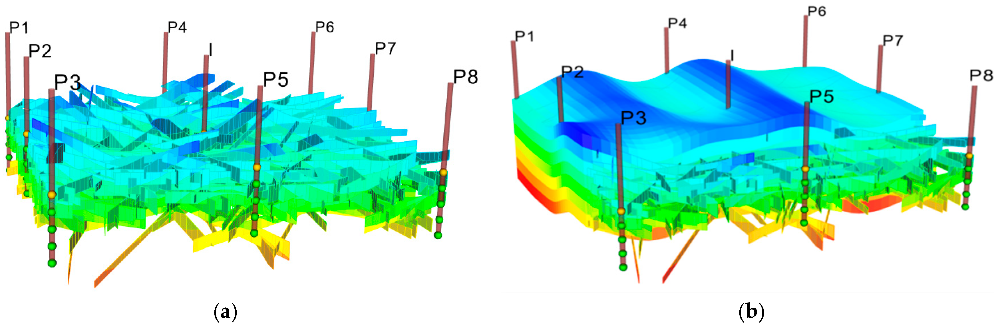
4.5. Comparison Using a Complex Fracture System

In this section, the objective is to test the robustness and the efficiency of the new approach in a complex fracture model. A gas injection simulation is performed on a complex fracture reservoir, and simulation results obtained from the new upscaling procedure and EDFM are compared.

The fracture system in Figure 20 is employed in the study. The model includes 41 × 41 × 7 matrix cells, along with 309 fractures. The matrix porosity is 0.10, and the matrix and fracture permeabilities are 0.1 mD and 5000 mD, respectively. Gas is pumped at a constant rate into the injection well, whereas the nine production wells are operating at a constant pressure. Figure 21 presents the simulation results of the gas–oil ratio and oil recovery for each producer. The gas–oil ratio curve shows a slight difference at the end of injection, and the recovery curve shows good consistency between the two methods. A slight difference gas–oil ratio is caused by the different relative permeability between fracture and matrix. However, the computation time for the new approach and for EDFM are 175 s, and 2560 s, respectively.

5. Conclusions

In this work, we implement a novel upscaling simulation method that uses EDFM to calculate equivalent permeability for a complex fracture network. The main objective of this work was to introduce the procedure and study the feasibility of this novel method. The new upscaling approach divides each cell into small cells and sets a constant pressure in flow directions and closed boundaries for the other two sides. Then, it uses EDFM to compute flow rate and applies the Darcy flow equation to calculate cell permeability. The proposed upscaling model was designed and compared with the DFM and EDFM methods, and comprehensive modeling studies were conducted to understand the key reservoir and fracture properties that affect upscaling performance. Both single-phase and multiphase flow were applied to investigate the feasibility of the new approach. We obtained the following conclusions from the simulation results:

(1)

The computation time of EDFM is much less than that of DFM in the shown model, which means that using EDFM to upscale permeability in a fractured reservoir would be more efficient than DFM.

(2)

For single-phase flow, the results obtained by the proposed upscaling approach, EDFM, and DFM (fine grid model) are close to each other in this study, which validates the proposed approach.

(3)

The recovery factor obtained by different methods has good consistency over the long term for multiphase flow. However, slight differences were found (for example, water cut curve and gas oil–ratio curve).

(4)

Grid number is an important parameter during the upscaling process. The calculated permeability tends to be uniform for each cell with an increase in meshes in the upscaling process.

In a forthcoming work, we will upscale relative permeability for fractured reservoirs with the EDFM method to describe the effects of reservoir heterogeneity on multiphase flow in simulation models, which could increase the efficiency and applicability of this method.

References

1. Hoteit, H.; Firoozabadi, A. Multicomponent fluid flow by discontinuous Galerkin and mixed methods in unfractured and fractured media. Water Resour. Res. 2005, 41, W11412. [Google Scholar] [CrossRef]
2. Nezhad, M.M.; Javadi, A.A.; Abbasi, F. Stochastic finite element modelling of water flow in variably saturated heterogeneous soils. Int. J. Numer. Anal. Methods Geomech. 2011, 35, 1389–1408. [Google Scholar] [CrossRef]
3. Karimi-Fard, M.; Durlofsky, L.J.; Aziz, K. An efficient discrete-fracture model applicable for general-purpose reservoir simulators. SPE J. 2004, 9, 227–236. [Google Scholar] [CrossRef]
4. Fumagalli, A.; Pasquale, L.; Zonca, S.; Micheletti, S. An upscaling procedure for fractured reservoirs with embedded grids. Water Resour. Res. 2016, 52, 6506–6525. [Google Scholar] [CrossRef]
5. Li, L.; Lee, S.H. Efficient field-scale simulation of black oil in a naturally fractured reservoir through discrete fracture networks and homogenized media. SPE Reserv. Eval. Eng. 2008, 11, 750–758. [Google Scholar] [CrossRef]
6. Hajibeygi, H.; Karvounis, D.; Jenny, P. A hierarchical fracture model for the iterative multiscale finite. J. Comput. Phys. 2017, 230, 8729–8743. [Google Scholar] [CrossRef]
7. Tene, M.; Al Kobaisi, M.; Hajibeygi, H. Multiscale projection-based Embedded Discrete Fracture Modeling approach (F-AMS-pEDFM). In Proceedings of the ECMOR Xv-15th European Conference on the Mathematics of Oil Recovery, Amsterdam, The Netherlands, 29 August–1 September 2016. [Google Scholar]
8. Matei, Ţ.; Kobaisi, M.S.A.; Hajibeygi, H. Algebraic multiscale method for flow in heterogeneous porous media with embedded discrete fractures (F-AMS). J. Comput. Phys. 2016, 321, 819–845. [Google Scholar] [Green Version]
9. Li, W.; Dong, Z.; Lei, G. Integrating Embedded Discrete Fracture and Dual-Porosity, Dual-Permeability Methods to Simulate Fluid Flow in Shale Oil Reservoirs. Energies 2017, 10, 1471. [Google Scholar] [CrossRef]
10. Barrenblatt, G.D.; Zheltov, I.P.; Kochina, I.N. Basic Concepts in the Theory of Homogeneous Liquids in Fissured Rocks. J. Appl. Math. 1960, 24, 1286–1303. [Google Scholar]
11. Warren, J.E.; Root, P.J. The behavior of naturally fractured reservoirs. SPE J. 1963, 3, 245–255. [Google Scholar] [CrossRef]
12. Pruess, K.; Narasimhan, T.N. A practical method for modeling fluid and heat flow in fractured porous media. SPE J. 1985, 25, 14–26. [Google Scholar] [CrossRef]
13. Snow, D.T. Rock fracture spacings, openings and porosities. J. Soil Mech. Found. Div. 1968, 94, 73–92. [Google Scholar]
14. Oda, M. Permeability tensor for discontinuous rock masses. Geotechnique 1985, 35, 483–495. [Google Scholar] [CrossRef]
15. Elfeel, M.A.; Geiger, S. Static and dynamic assessment of DFN permeability upscaling. In Proceedings of the 74th EAGE Conference & Exhibition, Copenhagen, Denmark, 4–7 June 2012. [Google Scholar]
16. Durlofsky, L.J. Upscaling of geocellular models for reservoir flow simulation: A review of recent progress. In Proceedings of the 7th International Forum on Reservoir Simulation, Baden-Baden, Germany, 23–27 June 2003; pp. 23–27. [Google Scholar]
17. Durlofsky, L.J. Upscaling and gridding of fine scale geological models for flow simulation. In Proceedings of the 8th International Forum on Reservoir Simulation Iles Borromees, Stresa, Italy, 20–24 June 2005. [Google Scholar]
18. Long, J.C.S.; Remer, J.S.; Wilson, C.R.; Witherspoon, P.A. Porous media equivalents for networks of discontinuous fractures. Water Resour. Res. 1982, 18, 645–658. [Google Scholar] [CrossRef] [Green Version]
19. Koudina, N.; Garcia, R.G.; Thovert, J.F.; Adler, P.M. Permeability of three-dimensional fracture networks. Phys. Rev. E 1998, 57, 4466. [Google Scholar] [CrossRef]
20. Kaufmann, G.; Romanov, D.; Hiller, T. Modeling three-dimensional karst aquifer evolution using different matrix-flow contributions. J. Hydrol. 2010, 388, 241–250. [Google Scholar] [CrossRef]
21. Lough, M.F.; Lee, S.H.; Kamath, J. An efficient boundary integral formulation for flow through fractured porous media. J. Comput. Phys. 1998, 143, 462–483. [Google Scholar] [CrossRef]
22. Bogdanov, I.I.; Mourzenko, V.V.; Thovert, J.F.; Adler, P.M. Effective permeability of fractured porous media in steady state flow. Water Resour. Res. 2003, 39, 1023. [Google Scholar] [CrossRef]
23. Lang, P.S.; Paluszny, A.; Zimmerman, R.W. Permeability tensor of three dimensional fractured porous rock and a comparison to trace map predictions. J. Geophys. Res. Solid Earth 2014, 119, 6288–6307. [Google Scholar] [CrossRef]
24. Fumagalli, A.; Zonca, S.; Formaggia, L. Advances in computation of local problems for a flow-based upscaling in fractured reservoirs. Math. Comput. Simul. 2017, 137, 299–324. [Google Scholar] [CrossRef]
25. Moinfar, A.; Varavei, A.; Sepehrnoori, K.; Johns, R.T. Development of an Efficient Embedded Discrete Fracture Model for 3D Compositional Reservoir Simulation in Fractured Reservoirs. SPE J. 2014, 19, 289–303. [Google Scholar] [CrossRef] [Green Version]
26. Ţene, M.; Sebastian, B.M.B.; Al Kobaisi, M.S.; Haijibeygi, H. Projection-based embedded discrete fracture model (pEDFM). Adv. Water Resour. 2017, 105, 205–216. [Google Scholar] [CrossRef]
27. Petrel. E&P Software Platform; Schlumberger: Sugar Land, TX, USA, 2014. [Google Scholar]
28. CMG. E&P Software Platform; Computer Modelling Group Ltd.: Calgary, AB, Canada, 2015. [Google Scholar]
29. Fracman. E&P Software Platform; Golder Associate: Bristol, UK, 2011. [Google Scholar]
Figure 1. A meshing example of embedded discrete fracture modeling (EDFM). (a) is the corner-point grid (2 × 2 × 2). (b) shows the two input intersecting fractures. (c) is the EDFM model.
Energies 12 00812 g001
Figure 2. An example of connection lists for EDFM. (a) shows the matrix grid and fracture distribution. (b) is the connection list. Reproduced from [Li et al.], publisher: 2017.
Energies 12 00812 g002
Figure 3. The fracture permeability upscaling procedure for fractured reservoirs.
Energies 12 00812 g003
Figure 4. The matrix grid and fracture distribution for a two-dimensional (2D) case. (a) is a matrix system of the corner-point grid (5 × 8), along with nine fractures. (b) shows an arbitrary grid from the left figure. The bottom-right figure shows the grid system for both the matrix and fractures after meshing the grid to 5 × 7.
Energies 12 00812 g004
Figure 5. The boundary condition for a new grid system shown in Figure 4b. Blue lines are fractures, green lines represent the constant pressure boundary, and thick black lines indicate closed (no flow) boundaries. In this case, the flow direction is from right to left or from left to right.
Energies 12 00812 g005
Figure 6. Connection information for the EDFM method for the cells shown in the red block of Figure 5. (a) shows four matrix cells with two fractures, with fracture one divided into segments F1 and F4 by matrix cells and fracture two divided into segments F2, F3, and F5 by matrix cells. (b) shows the connection among different media. Line colors represent the same elements as in Figure 2.
Energies 12 00812 g006
Figure 7. Fracture distribution for the EDFM and DFM model used in the study. (a) shows the fracture distribution, including 250 fractures with 5000-mD permeability and 0.01-ft aperture. (b) is the EDFM model, which presents fracture explicitly. (c) is the DFM model, which includes 238,762 cells.
Energies 12 00812 g007
Figure 8. A comparison of gas rate (a) and cumulative gas (b) between EDFM and DFM.
Energies 12 00812 g008
Figure 9. A conceptual model of fracture distribution and the EDFM and DFN model for one cell. (a) is the fracture distribution, including six fractures with 1000-mD permeability and 0.01-ft aperture. (b) is the EDFM model, and (c) is the DFN model.
Energies 12 00812 g009
Figure 10. A simple model with two cross-fractures used to validate the new approach. (a) shows the fractures, (b) is the fine grid model, which is used to represent fractures, and (c) is the EDFM.
Energies 12 00812 g010
Figure 11. The permeability upscaling result based on the new method. (a) shows the permeability distribution in the X direction, Kx, and (b) shows the permeability distribution in the Y direction, Ky.
Energies 12 00812 g011
Figure 12. A comparison of oil rate (a) and cumulative oil (b) for the new upscaling method, fine grid model, and EDFM model in a single-phase flow case.
Energies 12 00812 g012
Figure 13. A comparison of the pressure profile at the same time level for the new upscaling method, EDFM, and fine grid model in one-phase flow. The pressure figures for (a), (b), and (c) are the new upscaling method, EDFM, and fine grid model, respectively.
Energies 12 00812 g013
Figure 14. The fracture distribution and oil saturation profiles. (a) shows the fracture distribution for the model used in the study. (b) and (c) present upscaled permeability for the X and Y directions, respectively. The yellow lines in the figures represent fractures.
Energies 12 00812 g014
Figure 15. A comparison of oil rate (a) and cumulative oil (b) between the new upscaling model and EDFM.
Energies 12 00812 g015
Figure 16. Pressure profiles for different methods. (a) shows the pressure distribution for the new upscaling method model, and (b) and (c) show the matrix and fracture pressure distribution for EDFM. The pressure profile for the two methods is at the same time level. The blue line in the center of the model represents the producer.
Energies 12 00812 g016
Figure 17. The test domain with fractures and grid-blocks. (a) shows the domain with 14 fractures and an 11 × 11 grid-block. (b) represents a cell (5,3) with four fractures from the test domain, which would be subdivided into smaller cells. The bottom figures show four scenarios: (c) uses 5 × 5 grid-block to model one cell shown in figure (b), (d) 10 × 10 grid-block to model one cell shown in figure (b), (e) 15 × 15 grid-block to model one cell shown in figure (b), (f) 20 × 20 grid-block to model one cell shown in figure (b). Note that serial small cells are added to define the boundary condition in the study for each scenario.
Energies 12 00812 g017
Figure 18. A comparison of upscaling permeability with different grid-block numbers. (a) shows the upscaling permeability with different grid-block numbers for cell (5,3). (b) represents the upscaling permeability with different grid-block numbers for all cells.
Energies 12 00812 g018
Figure 19. A comparison of water cut (a) and recovery (b) for different methods in multiphase flow.
Energies 12 00812 g019
Figure 20. The fracture distribution and EDFM model used in the study. (a) is the fracture distribution, including 309 fractures with 5000-mD permeability and 0.01 ft aperture. (b) is the EDFM model, which presents fracture explicitly.
Energies 12 00812 g020
Figure 21. The simulation results of the gas–oil ratio (a) and oil recovery (b) for each producer.
Energies 12 00812 g021