Statistical Learning for Service Quality Estimation in Broadband PLC AMI


1
Department of Electronics Engineering, Hankuk University of Foreign Studies, Gyeonggi-do 17035, Korea
2
Department of Electronics and Information Engineering, Hansung University, Seoul 02876, Korea
*
Author to whom correspondence should be addressed.
Energies 2019, 12(4), 684; https://doi.org/10.3390/en12040684
Submission received: 12 January 2019
/
Revised: 6 February 2019
/
Accepted: 18 February 2019
/
Published: 20 February 2019
(This article belongs to the Section A1: Smart Grids and Microgrids)
Abstract
:In this paper, we propose a method to estimate communication performance for the advanced metering infrastructure that employs the power line communication (PLC) technology. Using bit-per-symbol signals from the PLC network management system, we estimate a PLC model quality in terms of packet success rate based on statistical learning. We also verify the accuracy of the estimations by comparing them with measured communication test results at test sites. Finally, from the packet success rate estimate, the qualities of services, such as meter readings and time-of-use pricing data downloading under several metering protocol sequences, are investigated through a mathematical analysis, and numerical results are provided.
1. Introduction
Advanced metering infrastructure (AMI) is a system composed of smart meters, communication networks, and systems for managing data. Utilities employ AMI to operate a variety of services and applications, such as meter reading of smart meters, remote management of smart meters, demand response (DR), provision of power information to the customer, and power distribution management [1]. From DR through AMI, the utilities can provide consumers with a variety of optional pricing rate information, such as the time-of-use (TOU), critical peak pricing, and real-time pricing, and can allow consumers to choose a reasonable pricing rate based on their power usage patterns [2,3,4].
An important challenge in constructing AMI is how to choose a cost-effective communication network that meets service requirements to deliver these services. Determining the field communication method for the network configuration in AMI is critical because the cost of building the communication network is very high [5]. As a field communication method for AMI, we can consider the power line communication (PLC) or wireless communication method. When adopting PLC methods, the configuration and the number of low-voltage customers using the same transformer are closely related to the communication quality as well as the AMI construction and operation cost. European utilities prefer PLC methods for the field communication because dozens to hundreds of low-voltage customers are connected to pad-mounted transformers through underground lines. On the other hand, in the United States, because typically less than 10 low-voltage consumers are connected to a pole-mounted transformer, utilities prefer wireless communications rather than PLC methods from the perspective of cost-effective construction and operation of AMI.
The technology on PLC methods can be classified into narrowband and broadband PLCs depending on the frequency bandwidth to be employed. Narrowband PLC generally yields low data rates due to the narrow bandwidth of 3–490 kHz. To overcome the limit of low rates and accommodate various service needs for utilities, powerline intelligent metering evolution (PRIME) and G3-PLC, which are based on the orthogonal frequency division multiplexing technology, have been introduced [6]. Broadband PLC uses relatively wide frequency bandwidth of 2–30 MHz compared to the narrowband PLC case. Three worldwide standards have been established as ITU-T G.hn, IEEE P1901, and ISO/IEC12139-1 [7]. Please note that PLC has an advantage that no additional communication lines are required. However, it is known that the PLC channel state changes with time due to time-varying characteristics of the power lines that are connected to various electrical equipment [8,9,10,11]. Signal attenuations are even larger when passing transformers. Hence, stable performance for data transmissions is not guaranteed in general. When the channel state of PLC deteriorates greatly, to reduce the communication error rate and thus improve the communication reliability, PLC tries to apply a strong forward error correction and repetitive transmissions in a diversity (DV) mode [7]. The DV mode employs a Reed-Solomon coder followed by diversity mapper. To efficiently manage large-scale PLC AMI networks in various and time-varying channel environments, a network management system (NMS) has been introduced and is in operation.
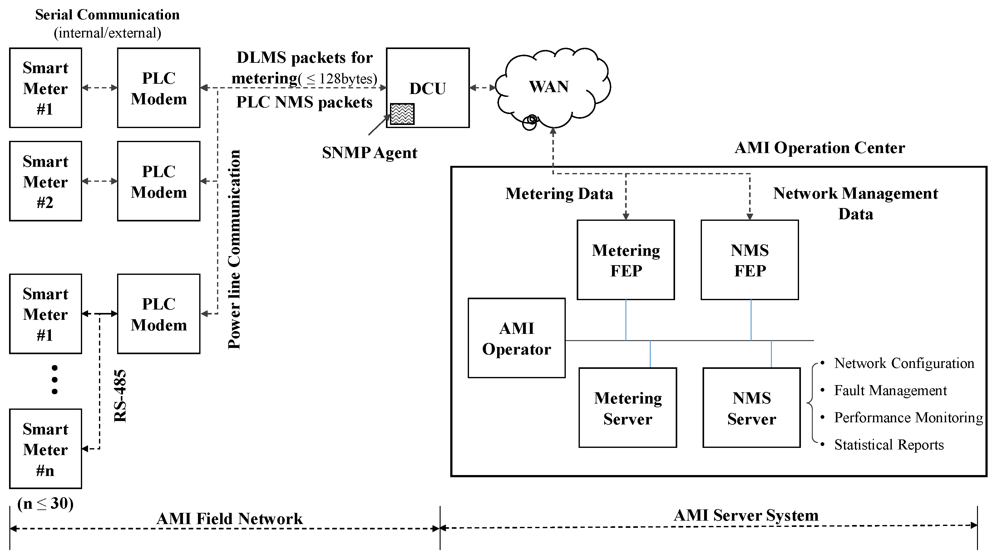
In Korea, most low-voltage customers are supplied with power through pole-mounted transformers, and on average, dozens of customers are connected to a transformer. Korea Electric Power Corporation (KEPCO), a Korean power company, adopts a broadband PLC (ISO/IEC12139-1 standard) [7] as an AMI field communication method in downtown residential areas, and adopts wireless communication methods, such as the smart utility network (SUN:IEEE 802.15.4g) [12] at 970 MHz and ZigBee (IEEE 802.15.4) [13] at 2.4 GHz, in rural areas. Home Plug Green PHY (HPGP) [14], a broadband PLC technology, is being adopted in downtown areas that are powered by underground lines. KEPCO has a plan to build AMI networks for 22.50 million low-voltage customers until 2020 [15,16]. The KEPCO AMI system, which is based on PLC, is composed of the AMI field network and AMI server system as shown in Figure 1. The data concentration unit (DCU) and PLC modem are used to construct the AMI field network, in which at least 200 smart meters can be supported by the corresponding DCU. PLC modems can be classified as an internal type embedded in a separate space of the smart meter and an external type connected with up to 30 smart meters through RS-485. DCU collects packets of the device language message specification (DLMS) from smart meters through PLC modems as shown in Figure 1. DCU then transmits metering data to the AMI server system. The AMI server system consists of metering and NMS servers, in which each server is connected to the front-end processor (FEP), a dedicated processor designed for communication controls. The metering FEP performs sending and receiving packets, and detecting and correcting packet errors between the metering server and the field DCUs. The NMS FEP performs communication tasks related to a network management between the NMS server and the simple network management protocol (SNMP) agent of DCU as shown in Figure 1. Here, the SNMP agent exchanges network management information with PLC modems to provide AMI network management functions, such as modem registration, modem repeating, bits-per-symbol (BPS) information collection, and modem firmware upgrade. NMS also periodically collects the BPS signal from PLC modems as a performance indicator to monitor the PLC channel condition. If the PLC channel is in a good condition, the BPS value goes up and vice versa.
To extend the field communication coverage between a target modem and the corresponding DCU, the communication path between the modem and DCU can be constructed with several different modems as shown in Figure 2. DCU collects information on BPS signals and hop numbers from PLC modems, and establishes links between PLC modems so that the communication state is good, and the number of hops is low. If a PLC modem cannot communicate with its parent PLC modem for a certain period of time, the PLC modem broadcasts a packet requesting a new path setup. For the conventional NMS, the communication condition of a target modem can be monitored from ping utility based on the internet protocol (IP) address. On the other hand, for the current NMS of KEPCO, each PLC modem can only access one-hop BPS signals between the modem and its parent based on the media access control address [17]. Hence, using such BPS signals, which are available from the given modem, is not sufficient to reflect the multiple modems in evaluating the communication path between the target modem and the DCU. Therefore, developing an evaluation algorithm for a modem communication condition using such one-hop BPS signals is required for the current KEPCO NMS.
In this paper, we propose a method to estimate the communication performance from the target modem to the DCU using the local BPS signals along the communication path based on a statistical learning. The proposed algorithm estimates the packet success rate (PSR) between the given modem to the corresponding DCU using a learned polynomial regression function incorporating linked BPS signals that are obtained along the path of the packets. Here, we use the PSR estimate as a communication quality of the modem. In addition, we use the PSR estimate to evaluate service qualities including the metering success rate (MSR) and the downloading success rate (DSR).
This paper is organized in the following way. In Section 2, 20 features from the one-hop BPS signals are introduced and then a PSR estimate algorithm using the features is proposed based on a statistical learning to observe a modem quality. Using the estimated PSR values, an AMI service quality is analyzed based on various service models in Section 3. Using BPS signals obtained from test sites of the Republic of Korea, the qualities of the modems of AMI network and AMI services were evaluated numerically in Section 4. The conclusion is then stated in the last section.
2. PLC Modem Quality Estimation
For a given PLC modem of AMI network as a target modem, we can only access the one-hop BPS signals as mentioned in the previous section. Using these one-hop BPS signals, we can construct the following BPS signals.
- Local BPS signals between the target modem and its parent modem
- Link BPS signals between the target modem and the corresponding DCU
In the local BPS signals, which are equivalent to the one-hop BPS signals, the uplink signal can be obtained from the parent of the target modem, where the amount of received data from the target modem is calculated, and the downlink signal from its parent can be calculated in the target modem. On the other hand, to obtain the link BPS signals, we first find the path that connects the target modem to the corresponding DCU. We then obtain the link BPS signals from combining all one-hop BPS signals that belong to the path. In this section, we first introduce various BPS features extracted from the BPS signals to describe data communication performance between PLC models and the corresponding DCU. We then define a modem quality that can describe communication states, and propose an estimate algorithm for the modem quality based on statistical learning.
2.1. BPS Features Extracted from the BPS Signals
Consider a weakly stationary sequence , for , with its expectation , for a given date of , where . Here, is the number of days for the sequence and is the data size per day. Let denote the uplink local BPS signal for the date of m. In a similar way, we can define the downlink local BPS signal as . Please note that these local BPS signals can be obtained from the parent of the target modem.
For evaluation of the modem quality, we first consider the following basic BPS features (F1–F6):
- F1 (UbMax), F4 (DbMax): maximal local BPS signals per day for uplink and downlink
- F2 (UbAvg), F5 (DbAvg): average local BPS signals per day for uplink and downlink
- F3 (UbMin), F6 (DbMin): minimal local BPS signals per day for uplink and downlink
Here, the maximum features F1 and F4 are defined as and , respectively. The average features F2 and F5 are defined as and , respectively. The minimum features F3 and F6 are defined as and , respectively. We can notice that the average features F2 and F5 for a given date can indicate the amount of data transmitted on average between modems. We have a total of 6 features of these basic features for both uplink and downlink as intuitive indicators for the communication performance.
The BPS signal can fluctuate depending on the link performance. The power spectral density [18] of the BPS signal can represent such variations versus frequencies. We call this power spectral density the noise power spectrum (NPS) of BPS signals. Let , for , denote the autocovariance function of , for a given data of m. Let , for , denote the -point discrete Fourier transform (DFT) of . then implies the NPS of for the uplink case, where is the sampling period of the BPS signal. Hence, the NPS of , which is denoted as , can be defined as [19,20]
In this definition for NPS, implies the number of frequency intervals. It should be large enough to include significant covariances in autocovariance function . To estimate NPS, we usually use an algorithm, which is called the Bartlett-Welch method [21,22], based on smoothing periodograms. We now formulate the Bartlett-Welch method to estimate NPS. Let denote -point DFT of . The periodogram of denoted as can be defined as . From the Bartlett’s procedure [21], we have the following convergence:
Hence, for periodogram-based direct method, the number of frequency intervals should be large enough to obtain unbiased or accurate NPS estimates. As additional features, we use normalized NPS (NNPS) values by the square of BPS average as for the uplink case. We can notice that the inverse of NNPS implies the square of the signal to noise ratio. For the downlink case, we can also define the NNPS values as with the expectation and the periodogram in a similar manner to the uplink case. Cumulative NNPS features (F7-F12) for different three frequency bands are then employed to provide a noisy property in the BPS signals as follows:
- F7 (UbPlow), F10 (DbPlow): low-band powers for uplink and downlink local BPS signals
- F8 (UbPmid), F11 (DbPmid): middle-band powers for uplink and downlink local BPS signals
- F9 (UbPhigh), F12 (DbPhigh): high-band powers for uplink and downlink local BPS signals
Here, using the uplink and downlink periodograms and , respectively, F7 and F10 are defined as and , respectively. F8 and F11 are defined as and , respectively. F9 and F12 are defined as and , respectively. We suppose that the BPS variation is low when the communication performance is good. It is then clear that small values of those 6 cumulative NNPS features imply a good communication performance.
For the local BPS signals, we can consider the zero BPS features (F13, F14) that are the numbers of zeros in the BPS signals for the target modem as follows:
- F13 (Uzero): Number of zeros in the uplink local BPS signal
- F14 (Dzero): Number of zeros in the downlink local BPS signal
When the communication performance is not good, the modem uses the DV mode and sets the BPS signals zero. Hence, the zero values in the BPS signals can imply a bad communication performance.
Several PLC modems construct a network including a gateway, which is called DCU, to transfer their metering data to a server through the gateway. To transfer metering data for the target modem, several modems of the network can be used to relay the data to the corresponding DCU as shown in Figure 2. The link BPS features (F15-F20), which use the link BPS signals along the route, can be summarized as follows:
- F15 (ULbMax), F18 (DLbMax): maximal link BPS features for uplink and downlink
- F16 (ULbAvg), F19 (DLbAvg): average link BPS features for uplink and downlink
- F17 (ULbMin), F20 (DLbMin): minimal link BPS features for uplink and downlink
These link BPS features (F15–F20) can describe communication performance between the target modem and the corresponding DCU. In the proposed approach of this paper, we incorporate this link BPS features to further accurately evaluate communication performance.
2.2. Polynomial Regression for Estimating the Modem Quality
To evaluate the communication performance of the modem, the PSR values, which are obtained from ping tests in the DCU, can be used. Here, PSR is a success rate for data transmission between the target modem and the corresponding DCU. For the target modem, we suppose that this PSR implies a modem quality with a value between 0 and 1. However, current NMS does not supply log data on such PSR values as mentioned in the introduction section. Hence, an algorithm for the PSR estimation is introduced in this section.
Appropriately using the introduced 20 features (F1–F20), which are extracted from BPS signals, we can estimate the PSR values of a given PLC modem. To design an algorithm for estimating PSR, we conduct statistical learning based on the polynomial regression [23,24] using the introduced 20 features and the PSR data. Here, the PSR data can be obtained by implementing a special PSR measurement program into DCU in a restrict environment for acquiring a training sequence (TS). Suppose that we have samples of PSR, i.e., the TS size is . An example of the second-order polynomial regression for , which denotes the i-th sample of PSR, can then be expressed as
for , where are called parameters and errors. Here, denotes the i-th sample of the j-th feature. Once the statistical learning is conducted for TS, we can then use the trained regression function to estimate the PSR for a given PLC modem. In the example of (3), instead of using all 20 features, we can use a subset of the features to simplify or optimize the estimation algorithm. We can also change the polynomial order to improve the regression performance. Conventional approaches are based on observing the BPS features of F1-F14, which are extracted from the local BPS signals. In the proposed approach of this paper is based on incorporating the link BPS features of F15-F20. In the experimental section, different parameters were tested for the polynomial regression using a TS and a comparison was shown for the proposed approach.
For a given DCU, we can use the average of the PSR values that belong to the DCU to evaluate the communication performance of the AMI network that contains the DCU. Hence, we can define the average as the DCU quality to represent a performance of AMI network.
3. Service Quality Analysis
In Korea, various metering methods, such as regular metering and LP metering, are being used based on PLC technology. The regular metering is for the monthly billing of electricity usage. On the other hand, the purpose of the LP metering lies in gathering other information about energy consumption. The TOU pricing is a method to reflect the cost of producing electricity, which varies hourly on a day [4]. For the TOU pricing to be in service, the TOU data need to be downloaded to each meter. The TOU pricing is planned to be in service in the near future in Korea. In this section, from the PSR introduced in the previous section, service qualities of metering and download for the TOU pricing are analyzed in terms of their success rates. We assume that each packet transmission is statistically independent of each other and has the same success probability. In addition, since the metering and download packets are transmitted very sparsely, packets rarely collide with each other. Thus, we do not consider the packet collision in the following analysis.
3.1. Metering Success Rate
There are two types of metering: regular and LP metering. For the monthly billing of electricity use, the regular metering tries to collect the metering data seven times every hour from 12 a.m. to 6 a.m. on a predetermined day. It is then regarded as a success when the metering data is received successfully once or more than once among the seven trials. The LP metering tries to collect the metering data four times in an hour with a 15-min period. In a similar manner to the regular metering case, in the LP metering, it is regarded as a success if at least one metering data is received. This kind of repeated data transmission scheme is employed to obtain a better meter reading performance. In a meter reading, 6 to 10 packet transmissions occur at an application layer that employs the DLMS protocol. The size of each packet can change depending on the type of the packet. However, since the packet size difference is not large, we assume that the PSR has a same value irrespective of the packet size. Now, let us denote PSR or the probability that a packet is successfully transmitted as p. The packet error probability, which is denoted as q, is then . Since the size of the metering data is very small as well as the number of nodes on the network, we can ignore their collisions. Thus, we can assume that packet errors are mainly caused by channel noise and interference induced from electrical loads.
Assume that the metering data consists of K packets and each packet can be retransmitted times, with M total transmissions possible. We also assume that the packet error probability does not change during the retransmissions and error events at each retransmission occur independently. The probability P that the first packet is received successfully with possible retransmissions is then given as Assuming that the errors of K packet transmissions are statistically independent from each other and the packet error probability q does not change, the probability of successful data transmission is and thus the probability that a meter reading fails is given as
Supposing there are N meter reading trials, we now derive the MSR for the regular and LP metering. Since there are relatively long intervals between the successive meter readings, it is assumed that the unsuccessful transmissions are statistically independent. Then, with N trials of meter reading, the probability that all the meter readings fail is from (4). Thus, the metering success probability or MSR is given as
3.2. Download Success Rate
Downloading data, such as the TOU pricing data, is potentially an important service of AMI. The TOU pricing data is downloaded irregularly and very rarely, i.e., once or twice a year. The typical size of the TOU pricing data in Korea is 10 kbytes and a packet is 128 bytes long [25,26,27]. Thus, the whole data consists of 80 packets. When a data transmission is not completed due to a bad channel condition, at every hour downloading resumes just after the data that have been received successfully. This process is done for up to a month. At the beginning of packet transmission, a header of 1 kbyte, which corresponds to 8 packets long, is transmitted before the pricing data. This header is also transmitted when a resumed download begins after a stopped download.
We now derive the probability that a download is completed successfully to obtain the DSR. Since the derivation is rather complex, we derive it in two steps as follows. First, the probability of successful download when the header packets are received without errors. The probability of the general case is then derived.
- Step 1: No errors in header packets are present.
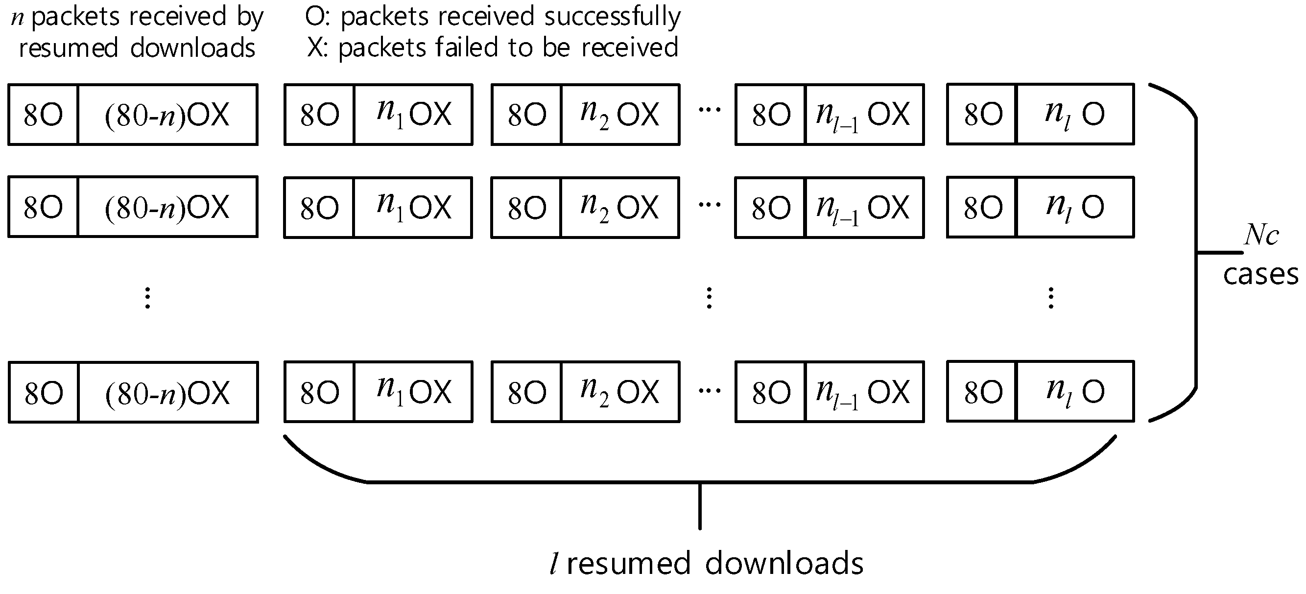
Assume that n packets are to be received by ℓ resumed downloads, where . Then packets are received successfully at first transmission. The remaining n packets are received through ℓ resumed downloads. Figure 3 shows the cases where n packets are transmitted through the ℓ resumed downloads when no header packets are in error. In this figure, each box represents a sequence of packets, in which “O” means a successful packet and ” X” packet in error. In addition, “nOX” represents n packets are received successfully, and the last packet is not received successfully. In Figure 3, a box with “8O”, appearing ahead of the other box represents 8 header packets received successfully. In each line, the probability of successful download is given as
where P is defined before (4) and . In (6), it is assumed that a packet in error can be retransmitted up to times. There are many cases that n packets can be downloaded with ℓ resumes. We denote the number of the cases as . In each line of Figure 3, at each resumed download segment, zero or more data packets can be a successful transmission, except the last segment. The last segment should have at least one successful packet. Otherwise, the number of resumes should be larger or smaller than ℓ. Let , , be the number of data packets at the i-th resumed download segment. Then,
holds. As mentioned previously, , should be a nonnegative integer and a positive integer. The number of all possible solutions which meet (7) is .
Now, let us find the value of . In Figure 3, each line has n circles and crosses after the first segment. We can put crosses between circles. At the beginning of the circles, crosses can be put. However, at the end of the circles, crosses cannot be put. Thus, there are n locations where crosses can be put. Moreover, multiple crosses can be put between two circles. Then, the number of circles between two crosses is . At the beginning and at the end, the number of circles before the first cross and after the last cross is and , respectively. Finding the combinations of this problem is similar to those of stars and bars problem [28]. The combinations is then given as
for given n and ℓ. Then from (6), the probability that n packets are downloaded successfully with ℓ resumed downloads is given as
By summing along n, we can obtain the probability of success with ℓ resumed downloads, which is denoted as , as
Let be the number of total possible transmission trials. The number of downloads ℓ can be . Taking all possible ℓ into consideration, the probability of successful download when the header packets are received without error is then derived as
where is the probability of successful download without resuming, and is given as .
- Step 2: Errors in header packets are present.
Now, when any of the header packets fails to be received, the probability of a successful download is derived. We denote a sequence of packets with error free header as Segment S. In addition, Segment F represents a sequence of packets with headers in error. When a header packet is not received successfully, the following data packet fails to be downloaded. Figure 4 shows a situation that data downloading is completed with ℓ resumes, where successfully downloaded segments are present. Please note that between the Segments S or before the first Segment S, Segments F can be placed. Of course, one or more Segments F can be placed at the locations. At Segment F, since the header packets are not transmitted successfully, there is no downloaded data.
The probability that Segment F occurs, , is given as
When Segments S are present as in Figure 4, there can be k Segments F, where . The k Segments F can be placed at locations. Please note that Segments F can come one after another. The number of cases that k Segments F can be placed multiply at locations are found by a similar approach to obtain . The number of combinations is given as
Since the probability that k Segments F occur is , the probability that k Segments F are located at positions is . The number of Segments F, k, can be . Thus, when there are ℓ resumes and header packet errors are present, the probability that Segments F occur is given as
Combining equations (9) and (14), the probability that data of n packets are successfully received by ℓ resumed download is given as
Since n is the number of data packets obtained by ℓ resumed download, . Taking all the possible cases of n into consideration, we obtain the probability of successful download with ℓ resumes, as
Now, let us consider the case when all the packets are received without resuming, which is the case for . Segments F can be placed before Segment S, which comes last, and the number of Segments F can be . The probability for this case is
As mentioned previously, . Taking all possible cases of ℓ into consideration, the probability of successful download when the header packets are received in error is given as
Finally, the probability of the successful download or DSR is obtained by adding up the probabilities and as
4. Experimental Results and Discussions
In this section, to conduct the statistical learning to design an estimate of PSR, we used BPS signals acquired from 50 PLC modems of 5 DCUs in a Daejeon city area of the Republic of Korea as TS. We call this sequence Daejeon TS. A validation sequence (VS) was also constructed using BPS signals from 21 PLC modems of 3 different DCUs (Daejeon VS). This VS was used to test a robustness of the designed estimate under different statistical condition.
4.1. Packet Success Rate Experiments
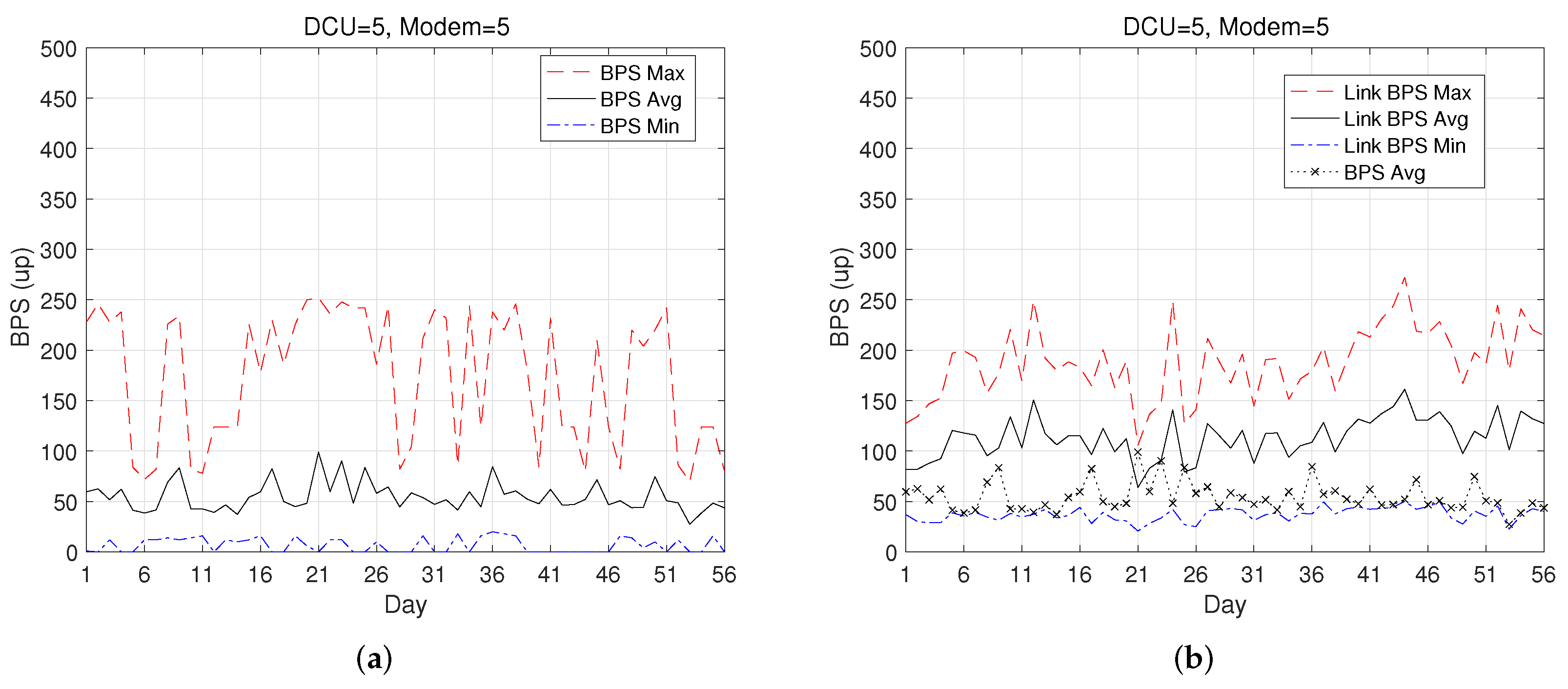
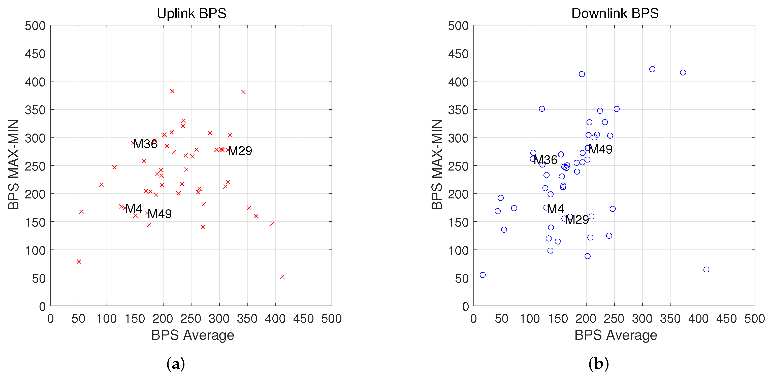
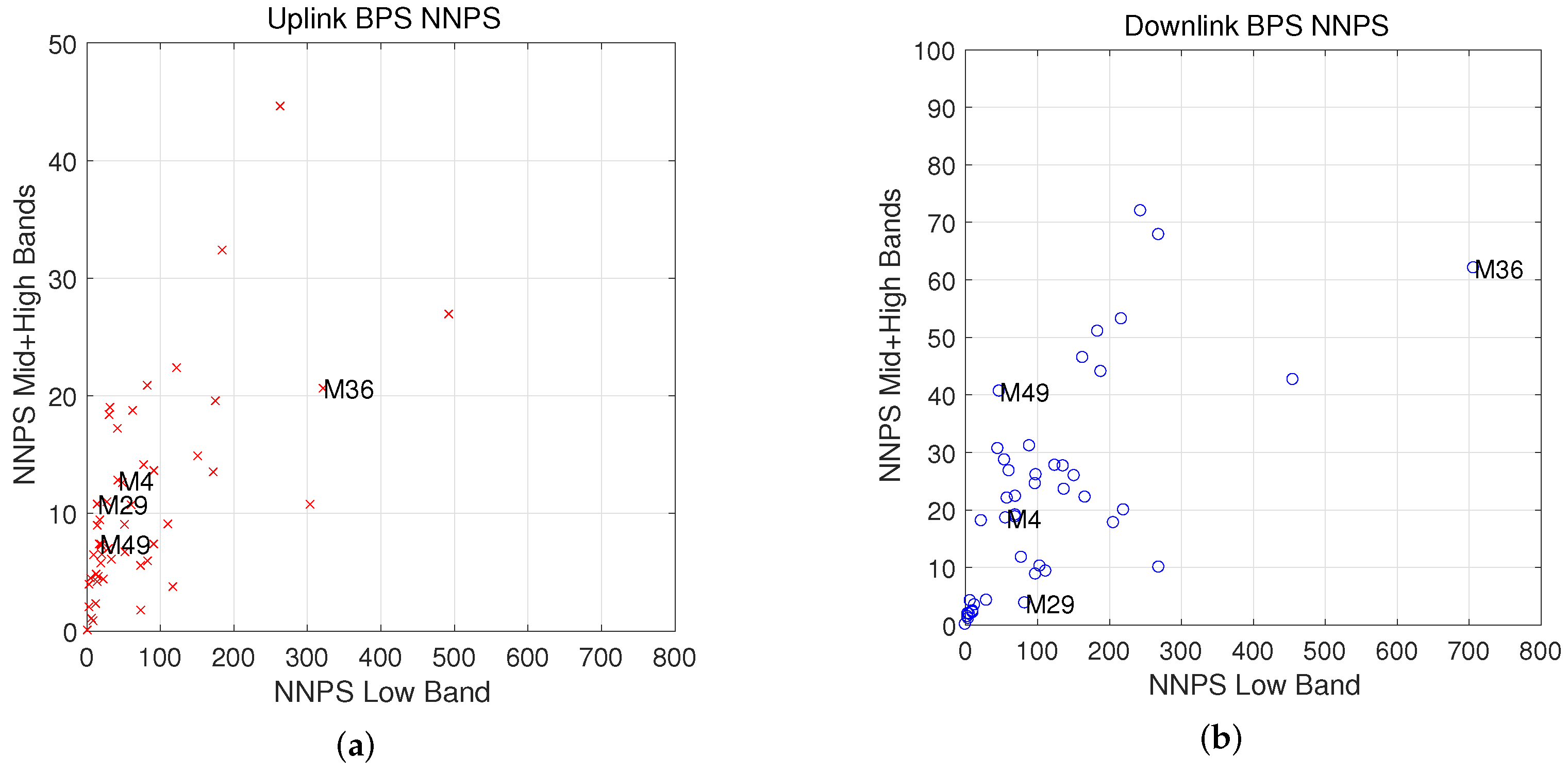
Figure 5 shows examples of the features extracted from the BPS signals of a PLC modem in Daejeon TS (Modem 5 of DCU 5). The average BPS signal per day (F2) shows values around BPS = 50. However, the maximal BPS signal per day (F1) has a relatively large variation as shown in Figure 5a. We can see from Figure 5b that the minimal link BPS (F17) is close to the average BPS (F2) of Figure 5a. In Figure 6, scatter diagrams of the basic BPS features (F1-F6) for Daejeon TS are illustrated for a better understanding of the basic statistical features of Figure 5a. It is believed that higher BPS average values (F2 and F5) can provide better communication performance for a given modem. Furthermore, smaller values of the differences |F1–F3| and |F4–F6| can provide more stable communication performance. For the uplink case of Figure 6a, Modem M4 showed the best basic BPS feature. From Figure 6, we can observe that the BPS features of the uplink and downlink cases are different. In Figure 7, scatter diagrams of the cumulative NNPS features (F7–F12) for Daejeon TS are illustrated for an observation of the feature values. The closer the feature value is to the origin, the better the communication performance of the modem. For the uplink case of Figure 7a as an example, Modem M49 showed the best NNPS feature.
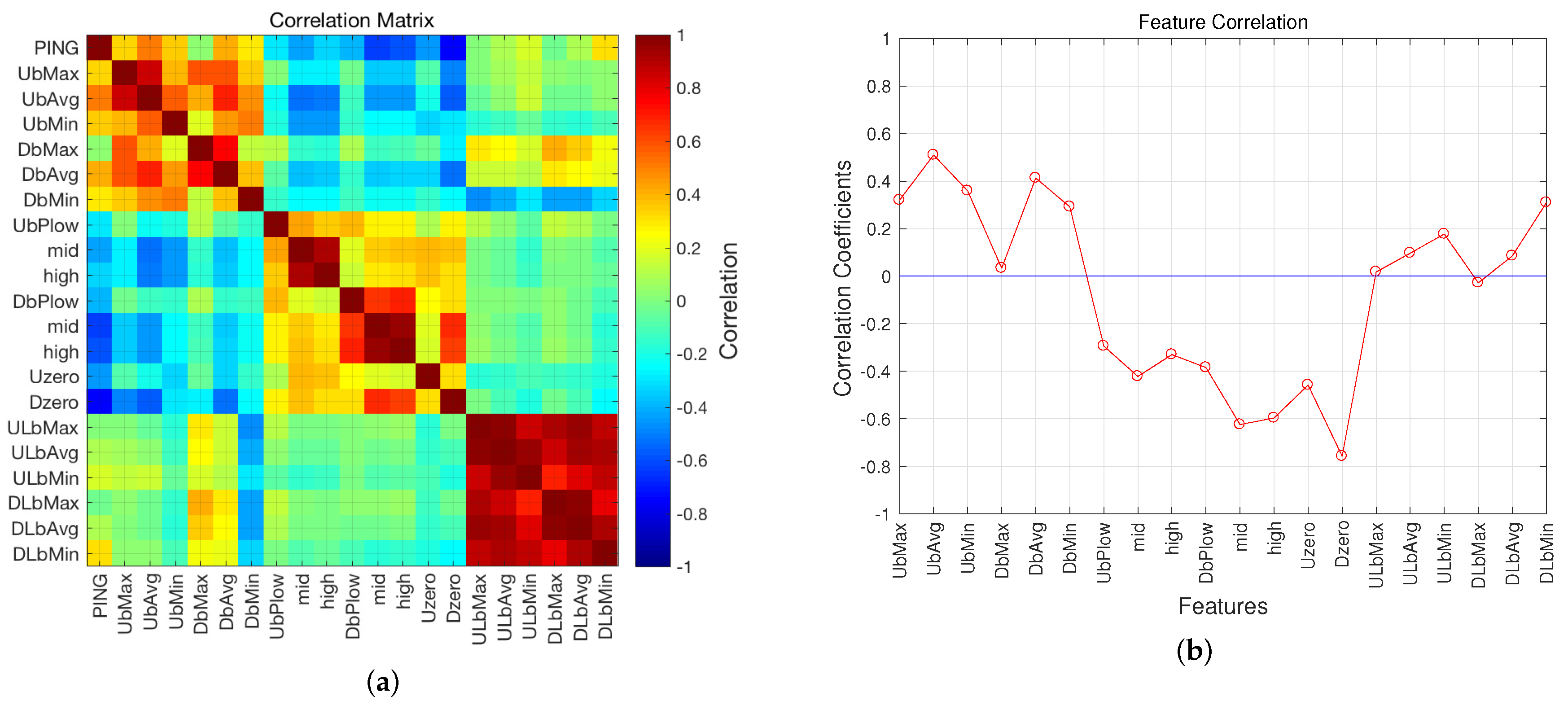
In Figure 8, a correlation matrix of the 20 features is illustrated to observe the cross-correlation coefficients between the features and measured PSR values. From observing this correlation matrix, we can select appropriate features for an estimation of PSR. We can observe that the NNPS (F7–F12; “UbPlow”–“DbPhigh”) and zero features (F13, F14; “Uzero” and “Dzero”) have relatively high correlations with PSR (Figure 8b). However, the link BPS features (F15–F20; “ULbMax”–“DLbMin”) show very low correlations (Figure 8b) and have a high correlation with each other (Figure 8a).
In Figure 9, the mean square error (MSE) values of both inside-TS and outside-TS versus different polynomial orders in statistical learning for the different feature combinations of “6F” (F1–F6), “12F” (F1–F12), “14F” (F1–F14), and “20F” (F1–F20) are depicted. Here, the leave-one-out cross validation technique was used for calculating the outside-TS MSE. A good learning shows a small difference of the MSE values of inside-TS and outside-TS [29]. We can notice from Figure 9 that the case of “20F” for the polynomial order of 2 showed the best estimation performance in terms of minimal MSE values.
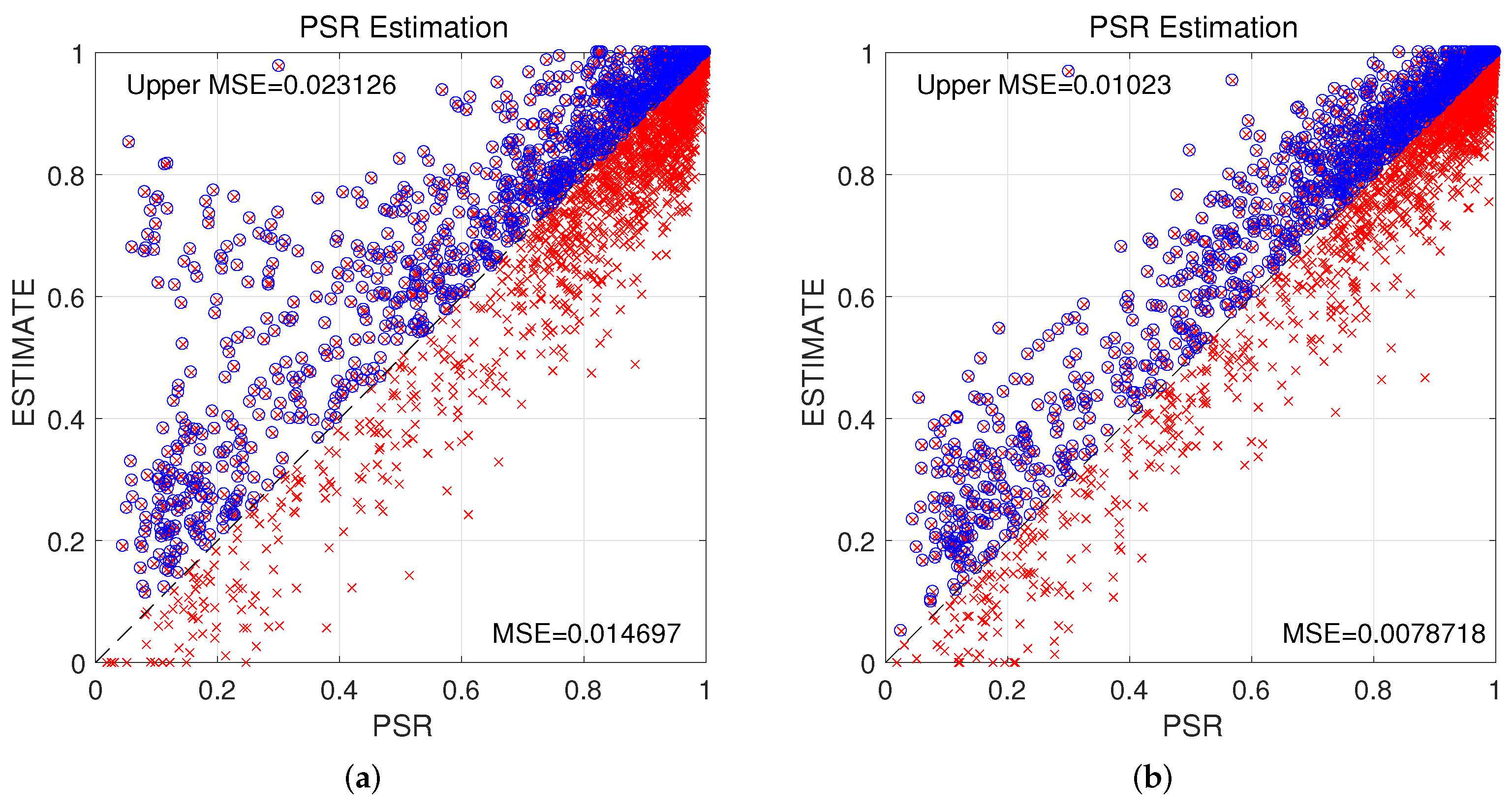
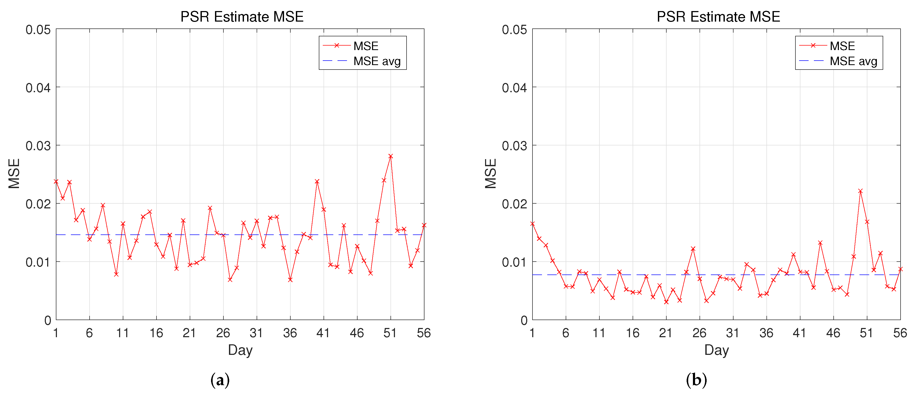
Figure 10 is a comparison of the scatter diagrams of the estimated PSR versus the true PSR. In the experiment of Figure 10, the estimates were conducted from a statistical learning based on the 3rd-order polynomial regression for Daejeon TS. We could see that the inside-TS MSE and the outside-TS MSE were very close with a difference of 0.15dB. When we did not use the link features as in the conventional approaches, the upper MSE (0.0231) was much higher than that of the lower MSE (0.0147) as shown in Figure 10a. In other words, estimating relatively low PSR values is difficult. However, incorporating the link features as in the proposed approach could reduce the upper MSE (0.0102), which was close to the lower MSE (0.00787), and could provide good estimates for low PSR values as shown in Figure 10b. Figure 11 illustrates the averages and standard deviations of PSR estimates compared to the true PSR values. Modem M49 in Figure 11b was an example of a low PSR value and showed an improved estimate precision due to the link features from Modem M49 of Figure 11a in the proposed approach. In Figure 12, the MSE values of estimate are compared for the cases of excluding and including the link BPS features (F15–F20). We can notice that using the link BPS features is very important in reducing the estimate errors.
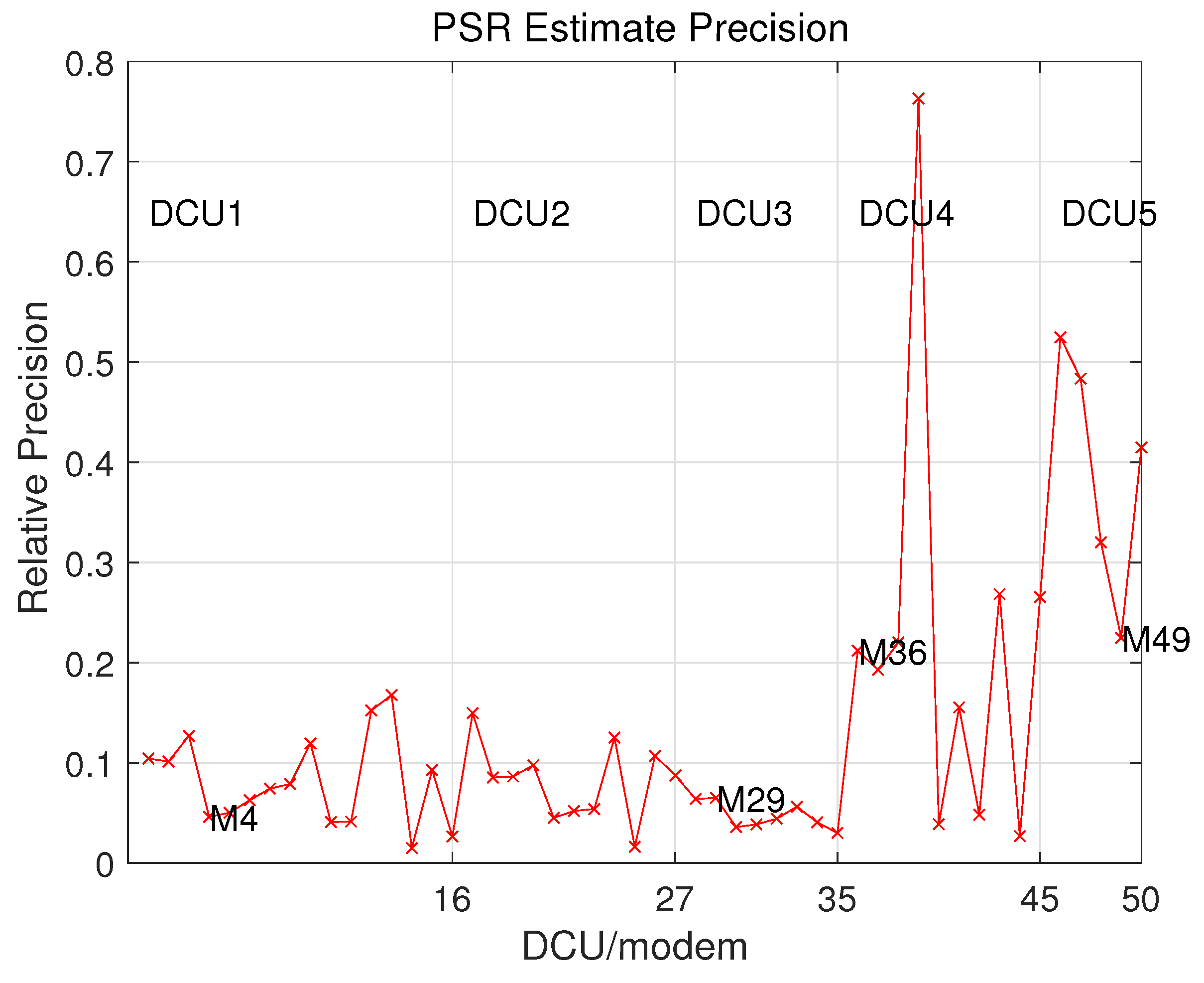
In Figure 13, the relative precision, which is defined as the standard deviation to mean ratio for PSR estimates, are illustrated. For the case of low values of PSR, the estimate precision is usually not good. This fact implies that estimation of relatively low PSR is more difficult than the relatively high PSR case as shown in Figure 11.
4.2. Metering Success Rate and Download Success Rate Experiments
For a meter reading, 6 to 10 packets are usually used. We choose the number of packets for a meter reading and let , meaning that each packet can be retransmitted up to 3 times. These are the typical values in AMI in Korea. For regular metering, meter readings are tried 28 times (), seven times a day for four days, while for LP metering, the number of tries is 4 () for an hour.
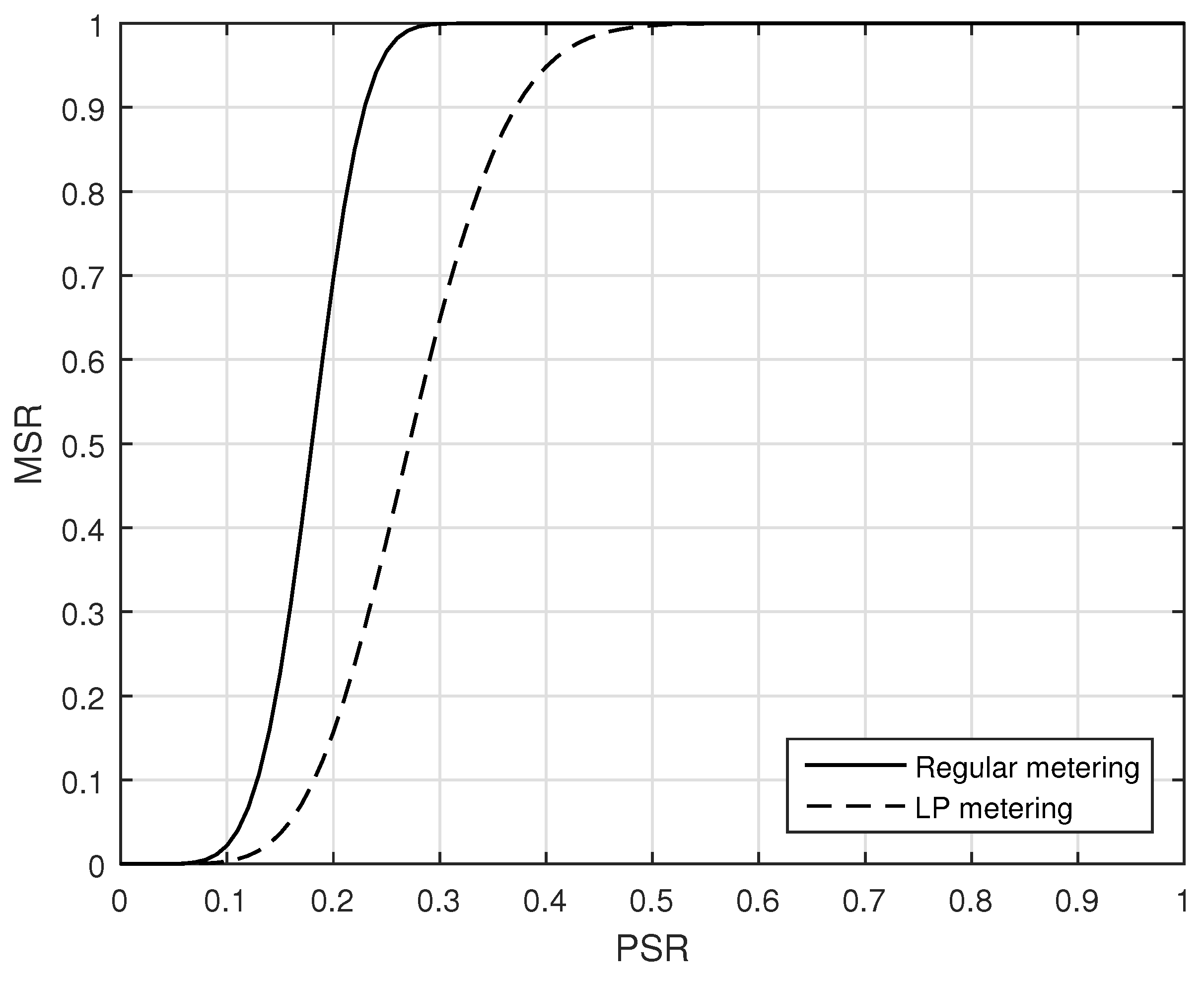
Figure 15 shows the results for the regular and LP metering. In this figure, the x-axis represents a PSR(or probability of a successful packet transmission) and y-axis the MSR. It is observed that with the same PSR, regular metering produces higher success rate. This is due to the lager metering trials at regular metering. From the results, it is observed that to achieve , the PSR should be equal to or greater than 0.24 for regular metering, while it should be equal to or greater than 0.40 for LP metering.
The typical parameters used for TOU pricing in Korea is as follows: TOU price data consists of 80 packets and in addition to these data packets, 8 packet long header is employed for a resumed download. When a packet is in error, the packet can be retransmitted up to 4 times, resulting . Resuming download is tried up to 24 times a day for 30 days, which means .
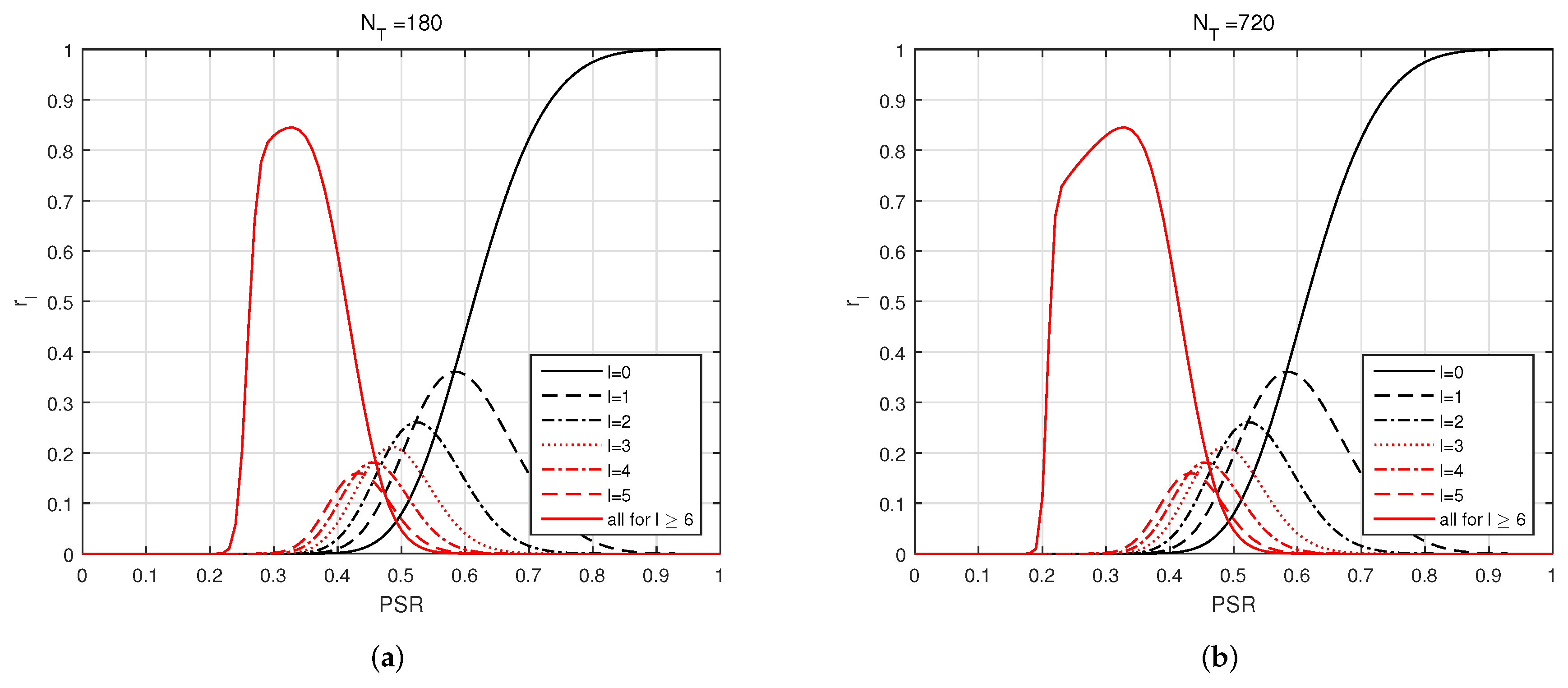
In the analysis of the successful download probability, and are derived. They are the probabilities of successful download at the ℓth resumed download. The former is the probability when no header packet error is present and the latter is the one that includes the case with header packets broken. Thus, represents the successful download probability at the ℓth resumed download. We let for simplicity. Figure 16a shows the results for at , when a PSR p is given. For , the probabilities are added up and the sum is shown. From the results, it is observed that at a high PSR, which means a low packet error rate, successful downloads are mainly achieved at , which is the case where the download is completed without resuming. However, as the PSR gets low, which means the higher packet error rate, the successful download is achieved at larger ℓ. In particular, it is seen that the sum of probabilities at has the largest value when the PSR is 0.33, which is a rather low PSR. This means that when a channel condition is bad, downloads are completed successfully with a lot of resumes. In this figure, was chosen to be 160.
Next, is increased to 720. The results are shown in Figure 16b. These results show little difference from those of Figure 16a when the PSR is greater than 0.3. Also, the sum of probabilities at has the largest value when the PSR is 0.33. The sum of with is larger than that with when the PSR is equal to or less than 0.3. This means that when the number of resumes is increased, the DSR can be improved at low p with the increased resume tries.
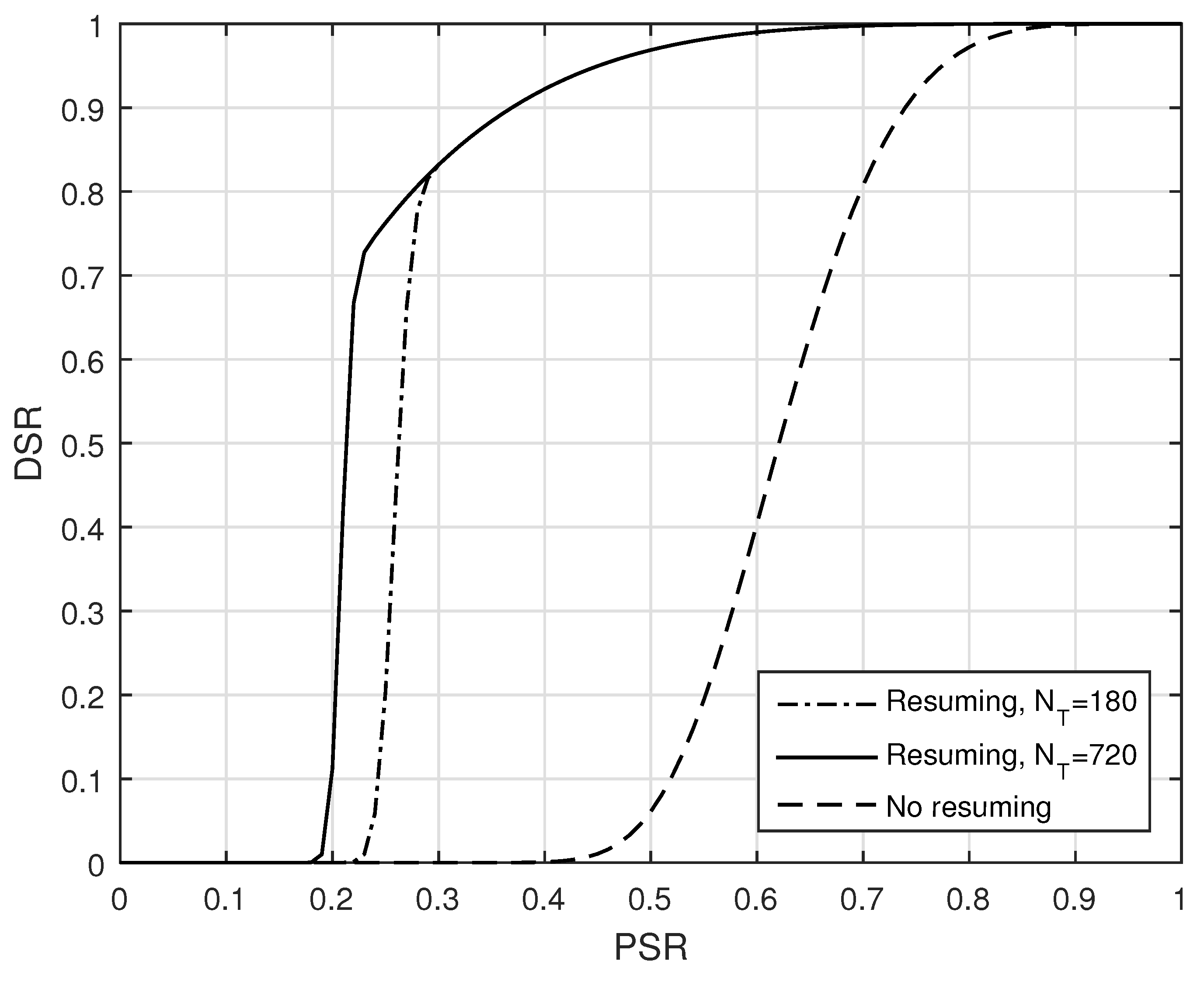
Finally, the results for the download success probability or DSR are shown in Figure 17 when = 160, 720. As seen previously, when the PSR is greater than 0.3, the DSR with shows no difference from the one with . Also in this figure, the DSR when a resume capability is not employed is shown for comparison purposes. From the results, we can observe that to obtain the DSR of 0.9, a PSR of 0.37 is needed when resume capability is employed, while 0.74 is required when a resume capability is not employed.
5. Conclusions
AMI system, which is an important part of the smart grid, should be constructed and operated in a way that is best suited to utilities, taking the site and service environment of each utility into account. KEPCO, a Korean power company, has adopted a broadband PLC for AMI, and is constructing nationwide AMI systems. To effectively establish and manage AMI systems, NMS for PLC AMI systems has been introduced and designed for evaluating the PLC modem quality based on the one-hop BPS values. In this paper, we first proposed a method to estimate communication quality of PLC modems in AMI systems based on statistical learning. Employing link BPS values along the path between the target modem and the corresponding DCU, we could improve the estimate accuracy from the mean square errors of 0.0146 to 0.0077 for a practical data set. The qualities of services including meter readings and TOU data downloading were then investigated through a mathematical analysis. When a PSR was given, analysis and experimental results for the LP MSR, regular MSR, and TOU data DSR were provided. From the results, we can observe that to achieve an MSR greater than , the PSR should be greater than 0.24 for regular metering.
Author Contributions
D.S.K. conducted the statistical leaning based on the polynomial regression and organized and refined the manuscript. B.J.C. derived the issues of communication and service quality management, and checked the validity of the prediction results. Y.M.C. conducted the service quality analysis and obtained the service quality experimental results.
Funding
This research was supported by grant No. CX 74170031 from the Korea Electric Power Corporation (KEPCO). This research for Young Mo Chung was financially supported by Hansung University.
Conflicts of Interest
The authors declare no conflict of interest.
Nomenclature
| AMI | Advanced metering infrastructure |
| BPS | Bit-per-symbol |
| DCU | Data concentration unit |
| DLMS | Device language message specification |
| FEP | Front-end processor |
| LP | Load profile |
| MSR | Metering success rate |
| DSR | Download success rate |
| NMS | Network management system |
| NNPS | Normalized NPS |
| NPS | Noise power spectrum |
| PLC | Power line communication |
| PSR | Packet success rate |
| SNMP | Simple network management protocol |
| TOU | Time-of-use |
| TS | Training sequence |
| VS | Validating sequence |
| , | Uplink and downlink NPS values |
| Number of days | |
| TS size | |
| Data size per day | |
| , | Autocovariance function of the uplink and downlink BPS signals |
| , | Power spectrum density of the uplink and downlink BPS signals |
| , | Periodogram of the uplink and downlink BPS signals |
| The i-th sample of PSR | |
| Regression parameters | |
| The i-th error | |
| The i-th sample of the j-th feature | |
| p | Packet success probability |
| q | Packet error probability |
| M | Number of total packet transmission trials allowed |
| P | Probability that a packet is received successfully with retransmissions allowed |
| Q | Probability of packet error with retransmissions allowed |
| K | Number of packets that compose a metering data |
| Probability that a single meter reading fails | |
| N | Number of meter reading trials |
| Metering success rate | |
| n | Number of packets to be downloaded |
| ℓ | Number of resumes |
| Combinations for n successful packet reception with ℓ resumes | |
| when no header packet in errors | |
| Combinations that Segments F are placed multiply at locations | |
| when a header packet in errors | |
| Probability of successful download with n and ℓ when header packets are not corrupted | |
| Probability of successful download when header packets are not corrupted | |
| Probability of successful download with n and ℓ when header packets are in error | |
| Probability of successful download when header packets are in error | |
| Number of total transmission trials allowed at downloading | |
| Probability of successful download with ℓ resumes | |
| Download success rate or probability of successful download |
References
- Uribe-Pérez, N.; Angulo, I.; de la Vega, D.; Arzuaga, T.; Fernández, I.; Arrinda, A. Smart grid applications for a practical implementation of IP over narrowband power line communications. Energies 2017, 10, 1782. [Google Scholar] [CrossRef]
- Palensky, P.; Dietrich, D. Demand side management: Demand response, intelligent energy systems, and smart loads. IEEE Trans. Ind. Inform. 2011, 7, 381–388. [Google Scholar] [CrossRef]
- Yu, T.; Kim, D.S.; Son, S.Y. Optimization of scheduling for home appliance in conjunction with renewable and energy storage resources. Int. J. Smart Home 2013, 7, 261–272. [Google Scholar]
- Hu, F.; Feng, X.; Cao, H. A short-term decision model for electricity retailers: Electricity procurement and time-of-use pricing. Energies 2018, 11, 3258. [Google Scholar] [CrossRef]
- Park, S.W.; Son, S.Y. Cost analysis for a hybrid advanced metering infrastructure in Korea. Energies 2017, 10, 1308. [Google Scholar] [CrossRef]
- Hoch, M. Comparison of PLC G3 and PRIME. In Proceedings of the 2011 IEEE International Symposium on Power Line Communications and Its Applications, Udine, Italy, 3–6 April 2011; pp. 165–169. [Google Scholar]
- International Organization for Standardization. Information Technology-Telecommunications and Information Exchange between Systems-Powerline Communication (PLC) Medium Access Control (MAC) and Physical Layer (PHY)—Part 1: General Requirements; ISO/IEC 12139-1; International Organization for Standardization: Geneva, Switzerland, 2009. [Google Scholar]
- Zimmermann, M.; Dostert, K. A multipath model for the powerline channel. IEEE Trans. Commun. 2002, 50, 553–559. [Google Scholar] [CrossRef]
- Zimmermann, M.; Dostert, K. An analysis of the broadband noise scenario in powerline networks. In Proceedings of the 2000 International Symposium on Power-Line Communications and its Applications, Limerick, Ireland, 5–7 April 2000. [Google Scholar]
- Gotz, M.; Rapp, M.; Dostert, K. Power line channel characteristics and their effect on communication system design. IEEE Commun. Mag. 2004, 42, 78–86. [Google Scholar] [CrossRef]
- Galli, S.; Scaglione, A.; Wang, Z. For the grid and through the grid: The role of power line communications in the smart grid. Proc. IEEE 2011, 99, 998–1027. [Google Scholar] [CrossRef]
- Chang, K.H.; Mason, B. The IEEE 802.15.4g standard for smart metering utility networks. In Proceedings of the 2012 IEEE Third International Conference on Smart Grid Communications (SmartGridComm), Tainan, Taiwan, 5–8 November 2012; pp. 476–480. [Google Scholar]
- Luan, S.; Teng, J.; Chan, S.; Hwang, L. Development of a smart power meter for AMI based on ZigBee communication. In Proceedings of the 2009 International Conference on Power Electronics and Drive Systems (PEDS), Taipei, Taiwan, 2–5 November 2009; pp. 661–665. [Google Scholar]
- HomePlug Alliance. HomePlug AV Specification Version 2.0; HomePlug Alliance: Beaverton, OR, USA, 2012. [Google Scholar]
- Korea Smart Grid Association (KSGA). Smart Grid Technology Trends Report; KSGA: Seoul, Korea, 2012. [Google Scholar]
- Kim, D.S.; Son, S.Y.; Lee, J. Developments of the in-home display systems for residential energy monitoring. IEEE Trans. Consum. Electron. 2013, 59, 492–498. [Google Scholar] [CrossRef]
- Kim, Y.I.; Park, S.J.; Jung, N.J.; Choi, M.S.; Park, B.S. Design and implementation of NMS using SNMP for AMI network device monitoring. In Proceedings of the 2016 IEEE International Conference on Power System Technology (POWERCON), Wollongong, Australia, 28 September–1 October 2016; pp. 1–6. [Google Scholar]
- Oppenheim, A.V.; Schafer, R.W. Discrete-Time Signal Processing, 3rd ed.; Pearson Education: Upper Saddle River, NJ, USA, 2010. [Google Scholar]
- Jenkins, G.M.; Watts, D.G. Spectral Analysis and Its Applications; Holden-Day: San Francisco, CA, USA, 1969. [Google Scholar]
- Papoulis, A. Probability, Random Variables, and Stochastic Processes, 3rd ed.; McGraw Hill: New York, NY, USA, 1991. [Google Scholar]
- Bartlett, M.S. Periodogram analysis and continuous spectra. Biometrika 1950, 37, 1–16. [Google Scholar] [CrossRef] [PubMed]
- Welch, P.D. The use of fast Fourier transform for the estimation of power spectra: A method based on time averaging over short, modified periodograms. IEEE Trans. Audio Electroacoust. 1967, 15, 70–73. [Google Scholar] [CrossRef]
- Sen, A.; Srivastava, M. Regression Analysis; Springer: New York, NY, USA, 1990. [Google Scholar]
- Hastie, T.; Tibshirami, R.; Friedman, J. The Elements of Statistical Learning: Data Mining, Inference, and Prediction; Springer: New York, NY, USA, 2001. [Google Scholar]
- Park, B.S.; Kim, B.J.; Myung, N.G.; Kang, S.G.; Jeon, G.S.; Cho, J.H.; Kim, D.S. Data Transmission Method for Electronic Watt-Hour System. Patent No. 10-2016-0038121, 26 September 2016. [Google Scholar]
- General Technical Specifications of KEPCO. Data Concentration Unit for Low Voltage Automatic Meter Reading; Korea Electric Power Corporation: Naju, Korea, 2012. [Google Scholar]
- General Technical Specifications of KEPCO. PLC Modem for Low Voltage Advanced Metering Infrastructure; Korea Electric Power Corporation: Naju, Korea, 2015. [Google Scholar]
- Feller, W. An Introduction to Probability Theory and Its Applications, 2nd ed.; John Wiley & Sons: New York, NY, USA, 1957; Volume 1. [Google Scholar]
- Kim, D.S.; Bell, M.R. Upper bounds on empirically optimal quantizers. IEEE Trans. Inf. Theory 2003, 49, 1037–1046. [Google Scholar]
Figure 1.
KEPCO AMI system based on PLC. DCU collects metering and NMS information data.

Figure 2.
Configuration example of AMI field network in KEPCO.

Figure 3.
Successful transmissions with ℓ resumes and no header packets in error.

Figure 4.
Header packets in errors are present.

Figure 5.
Example of BPS features (Daejeon TS, DCU 5, modem 5). (a) Basic statistical features (F1–F3; average, maximum, and minimum per day). (b) Link BPS features (F15–F17; average, maximum, and minimum per day).
Figure 5.
Example of BPS features (Daejeon TS, DCU 5, modem 5). (a) Basic statistical features (F1–F3; average, maximum, and minimum per day). (b) Link BPS features (F15–F17; average, maximum, and minimum per day).

Figure 6.
Scatter diagrams of the basic BPS features (F1–F6) for Daejeon TS. (a) Uplink of |F1–F3| versus F2. (b) Downlink of |F4–F6| versus F5.
Figure 6.
Scatter diagrams of the basic BPS features (F1–F6) for Daejeon TS. (a) Uplink of |F1–F3| versus F2. (b) Downlink of |F4–F6| versus F5.

Figure 7.
Scatter diagrams of the cumulative NNPS features (F7–F12) for Daejeon TS. (a) Uplink of F8 + F9 versus F7. (b) Downlink of F11 + F12 versus F10.
Figure 7.
Scatter diagrams of the cumulative NNPS features (F7–F12) for Daejeon TS. (a) Uplink of F8 + F9 versus F7. (b) Downlink of F11 + F12 versus F10.

Figure 8.
Correlations of the 20 features (F1-F20) extracted from the BPS signal and PSR (“PING”) of Daejeon TS. (a) Correlation matrix. (b) Correlations between the 20 features and PSR.
Figure 8.
Correlations of the 20 features (F1-F20) extracted from the BPS signal and PSR (“PING”) of Daejeon TS. (a) Correlation matrix. (b) Correlations between the 20 features and PSR.

Figure 9.
MSE versus the polynomial order in statistical learning for the different feature combinations of “6F” (F1–F6), “12F” (F1–F12), “14F” (F1–F14), and “20F” (F1–F20).
Figure 9.
MSE versus the polynomial order in statistical learning for the different feature combinations of “6F” (F1–F6), “12F” (F1–F12), “14F” (F1–F14), and “20F” (F1–F20).

Figure 10.
Comparison of scatter diagrams on PSR versus its estimate based on the 3rd-order polynomial regression (Daejeon TS). (a) Conventional approach: learning using F1–F14 without the link BPS features. Inside-TS MSE is −18.33 dB and the outside-TS MSE (leave-one-out cross validation) is −14.39 dB. (b) Proposed approach: learning using F1–F20. Inside-TS MSE is −21.04 dB and the outside-TS MSE (leave-one-out cross validation) is −19.87 dB.

Figure 11.
Modem quality comparison (PSR estimate for the modem of Daejeon TS). (a) Conventional approach: estimate designed excluding the link BPS features. (b) Proposed approach: estimate designed using the 20 BPS features as Figure 10. Modem M49 shows an improved precision due to employing the link features.

Figure 12.
MSE comparison in PSR estimate for Daejeon TS. (a) Conventional approach: estimate designed excluding the link BPS features (MSE average: 0.0146). (b) Proposed approach: estimate designed using the 20 BPS features as Figure 10 (MSE average: 0.0077).
Figure 12.
MSE comparison in PSR estimate for Daejeon TS. (a) Conventional approach: estimate designed excluding the link BPS features (MSE average: 0.0146). (b) Proposed approach: estimate designed using the 20 BPS features as Figure 10 (MSE average: 0.0077).

Figure 13.
Relative precision of the PSR estimate for Daejeon TS. Estimate designed using the 20 BPS features as Figure 10.
Figure 13.
Relative precision of the PSR estimate for Daejeon TS. Estimate designed using the 20 BPS features as Figure 10.

Figure 14.
DCU quality (PSR estimate average of the corresponding modems). (a) Daejeon TS with 5 DCUs and 50 modems (MSE average: 0.0077). (b) Daejeon VS (3 DCUs).
Figure 14.
DCU quality (PSR estimate average of the corresponding modems). (a) Daejeon TS with 5 DCUs and 50 modems (MSE average: 0.0077). (b) Daejeon VS (3 DCUs).

Figure 15.
Metering success rate.

Figure 16.
Probability comparisons at various ℓ. (a) . (b) .

Figure 17.
Download success rate.

© 2019 by the authors. Licensee MDPI, Basel, Switzerland. This article is an open access article distributed under the terms and conditions of the Creative Commons Attribution (CC BY) license (http://creativecommons.org/licenses/by/4.0/).
Share and Cite
MDPI and ACS Style
Kim, D.S.; Chung, B.J.; Chung, Y.M. Statistical Learning for Service Quality Estimation in Broadband PLC AMI. Energies 2019, 12, 684. https://doi.org/10.3390/en12040684
AMA Style
Kim DS, Chung BJ, Chung YM. Statistical Learning for Service Quality Estimation in Broadband PLC AMI. Energies. 2019; 12(4):684. https://doi.org/10.3390/en12040684
Chicago/Turabian StyleKim, Dong Sik, Beom Jin Chung, and Young Mo Chung. 2019. "Statistical Learning for Service Quality Estimation in Broadband PLC AMI" Energies 12, no. 4: 684. https://doi.org/10.3390/en12040684
Note that from the first issue of 2016, this journal uses article numbers instead of page numbers. See further details here.