Aggregate Control Strategy for Thermostatically Controlled Loads with Demand Response


1
State Key Laboratory of Advanced Electromagnetic Engineering and Technology, Huazhong University of Science and Technology, No.1037 Luoyu Road, Wuhan 430074, China
2
Yichang Power Supply Company, Hubei Power Supply Company of State Gird, 117 Yanjiang Road, Yichang 443000, China
*
Author to whom correspondence should be addressed.
Energies 2019, 12(4), 683; https://doi.org/10.3390/en12040683
Submission received: 5 January 2019
/
Revised: 16 February 2019
/
Accepted: 18 February 2019
/
Published: 20 February 2019
Abstract
:The improvement of intelligent appliances provides the basis for the demand response (DR) of residential loads. Thermostatically controlled loads (TCLs) are one of the most important DR resources and are characterized by a large load and a high degree of control. Due to its distribution characteristic, the aggregation of TCLs and their control are key issues in implementing the load control for the DR. In this study, we focus on air conditioning loads as an example of TCLs and propose a simple and transferable aggregate model by establishing a virtual house model, which accurately captures the aggregate flexibility. The deviation of the aggregate model is analyzed for the model evaluation. An air conditioning DR control scheme is proposed based on the aggregate model; it has the advantage of simple implementation and convenient control for the individual units. Simulations are performed in Gridlab-D to evaluate the accuracy and effectiveness of the proposed model and control method.
1. Introduction
Power consumers participate in the control and operation of power systems through the demand response (DR), which results in considerable benefits, such as improving the operation efficiency of the power system, reducing the cost of electricity, and even increasing the social benefits [1,2]. With the rapid development of advanced metering infrastructures and bidirectional communication, residential consumers can easily take part in the DR [3]. Thermostatically controlled loads (TCLs) such as air conditioning loads are one of the most important DR resources. The DR of TCLs can be applied in frequency regulations, capacity reserves, ancillary services, etc. Current research on TCLs and its DR has mainly focused on aggregate models and DR schemes.
The purpose of aggregate models of TCLs is to describe the probability density evolution of a population of TCLs. Many mathematical models have been used for this purpose such as regression models [4], physics-based models [5], stochastic Fokker–Planck diffusion models [6], partial differential equation (PDE) models [7,8], and Markov chain models [9,10]. These models are used to calculate the relationship between the control variables of TCLs and the change in the load level.
An additional research focus is the achievement of the DR. Lu et al. [11] presented a queueing model to analyze the DR based on price aggregate TCLs. Callaway [12] regulated aggregated homogeneous TCLs by changing the setpoint temperature. Bashash and Fathy [7] achieved the DR for homogeneous TCLs by setting changing rate of the setpoint temperature. Using on/off control signals, Lu and Zhang [13] regulated the number of running appliances by using a centralized direct load control strategy for continuous regulation reserves. Tindemans et al. [14] investigated a decentralized frequency-based control strategy of TCLs for flexible DR. Erdinç et al. [15] discussed different DR strategies for providing frequency regulation and compared the performance of experimental and simulation results. Hu et al. [16] proposed a hierarchical centralized control algorithm to provide DR service without affecting the customers’ comfort levels.
However, from a practical point of view, most of the models and schemes require advanced communication technology, which results in high costs for practical applications. Moreover, it is unlikely that a residential consumer, who is not a skillful grid operator, will implement a proposed plan for using electricity. Furthermore, it is impractical to require the appliances to accurately implement an external control command. Therefore, an aggregate model and control strategy, which is simple and easy to implement, is needed for the effective regulation of all TCL units.
In this study, we propose an aggregate model and DR control strategy for TCLs. First, a virtual house model capable of characterizing the relationship between the average temperature and the total power of a population of TCLs is established. Second, considering the interactions of a large number of heterogeneous TCLs, the deviation of this model is determined by comparing it with other detailed models. Within the allowable range, the difference in the heat exchange rate resulting from the indoor temperature difference between the TCLs can be ignored. Third, a DR scheme is proposed to achieve the load control and suppress the load rebound. Finally, a Gridlab-D simulation is performed to demonstrate the effectiveness of the proposed scheme. The main contributions of this paper are the following: (1) the proposed aggregate model has fast computation speed, which reduces the computation time and improves the server performance. (2) The proposed DR scheme achieves accurate load control without the need for individual difference control. (3) The proposed aggregate model and DR scheme are applicable to homogeneous models and heterogeneous models.
2. Modeling of Air Conditioning Load
In this section, the equivalent thermal parameters (ETP) model, which defines the temperature dynamics of the air conditioner is presented. To develop an aggregate model for air conditioners, we propose a virtual house model to approximate the relationship between power consumption and average indoor temperature. Based on this model, a DR scheme is put forward. It is worth mentioning that the virtual house model is only used for an approximate analysis and the deviation is presented in Section 5.
A. Physical model of air conditioning loads
The components of the air conditioning system include a compressor, condenser, fan, and other parts. The compressor cools the liquid by compressing the refrigerant (e.g., Freon); an endothermic reaction occurs and the liquid changes its state at atmospheric pressure [17]. Similarly, an air conditioning system can produce heat [18]. The deadband is an important parameter to consider in a thermostat [19]. An air conditioning thermostat is used to control the indoor temperature and is used to adjust the operating time constant of the air conditioning equipment to ensure that the indoor temperature remains within a given range.
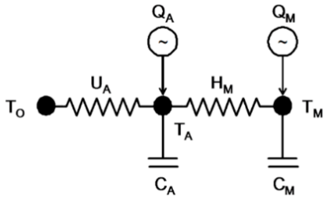
The heat flow between the inside of the house and the outside is a key factor affecting the air conditioning load. For a house, the following types of heat exchanges occur: (1) heat conduction through facades, roofs, and windows, (2) heat exchange due to indoor-outdoor airflow, (3) solar heat irradiating to the house directly (sun), and (4) heat generated by electrical equipment (internal gains) [20].
The thermal flow is shown in Figure 1.
As shown in Figure 1, we can obtain the expressions of the air temperature node and the wall temperature node:
Equation (1) [20] is solved for TM, differentiated with respect to time to provide dTM/dt, and both are substituted into Equation (2) to create a second-order linear differential equation in TA of the form:
where
, , ,
Thus, we can obtain an expression for TA:
where
The temperature, thermal mass, and heat flow in physics are equivalent to the voltage, capacitor, and current flow in an electric circuit. Therefore, a circuit relationship equivalent to the thermal relationship can be developed, as shown in Figure 2. In practice, this circuit is always overdamped. In other words, the temperature and load exponentially decay and approach steady-state (not oscillatory) conditions.
B. The virtual house model
In TCLs, aggregate load models are used to study the effects of DR control [7] or other special cases [21]. As mentioned above, many studies on aggregate models of TCLs have been conducted. Different aggregation methods have been used in these aggregate models depending on whether the goal was to improve the accuracy or an easy implementation of the load control.
From the perspective of economy and feasibility, in aggregate models, the independent control of a temperature controlled appliance (TCA) should be avoided. The requirement of independent control of each TCA means that control devices and instant communication devices have to be installed in each TCA. In fact, aggregate control of TCAs is often implemented in residential houses, shopping malls, dormitories, and hotels. In these situations, there is a strong consistency between every TCL. The scheme achieves DR of the aggregated TCLs using simple control signals. This type of scheme is proposed and is described next.
The aggregate model for achieving DR of the aggregated TCLs using simple control signals is developed by creating a virtual house that includes all TCAs. The virtual house ignores the state parameters of the aggregated units and calculates the total loads over a period by using only the initial state quantities and characteristic parameter values of the aggregated units. In other words, we propose a virtual house, in which the heat exchange with the outdoors is equivalent to the sum of the heat exchange of the aggregated units.
The virtual house is created using the following steps. A virtual house consisting of two houses is used as an example.
- Two houses have their own initial indoor temperatures and setpoints.
- We assume that there is a pipe with a switch between the two houses. There is no heat exchange between the pipe and the outside. If the switch is on, the pipe creates infinite heat exchange between the two houses. It is worth mentioning that this pipe does not exist in reality and is only used to understand the analysis.
- If the switch is on, the air temperatures inside the two houses are the same in the next unit of time. The two houses are equivalent to one virtual house and the area of the virtual house is the sum of the area of the two houses. The heat exchange coefficient with the outside world is equal to the sum of the heat exchange coefficients of the two houses. Although the coefficient of heat exchange is the same, the heat exchange between the virtual house and the outside is not strictly equal to the heat exchange between the two houses and the outside because of the indoor temperature difference.
- In Gridlab-D, this progress means establishing a house whose area is equal to the sum of the area of two small houses and modifying the corresponding heat exchange parameters to make them equivalent, as shown in Figure 3.
In the circuit equivalent model, the resistance and capacitance are parallel, as shown in Figure 3.
The virtual house model is expected to reflect the relationship between the average indoor temperature of the aggregate and the total load, which means that the heat exchange between the virtual house and the outside equals the sum of the heat exchange between each house and the outside. This needs to be verified by mathematical derivation.
3. Aggregate Model Validity Analysis
Two scenarios are created and analyzed to improve the accuracy of the proposed aggregate (virtual house) model and the effectiveness of the aggregated load control.
Scenario one: Homogeneous model
The homogeneous model consists of houses with the same areas, structures, and building materials. Assuming that there are house A1 and house A2, according to the ETP model, the following equation is obtained.
In the homogeneous model, a1 = a2 = … = an, the same applies to b, c, and d. Equation (5) can be simplified as.
Equation (6) has the form of a second-order linear differential equation for TA (Equation (3)). Therefore, the virtual house is equivalent to all houses. Similarly, a virtual house can be equivalent to several houses with the same structure but different area.
In this case, the initial temperature of the equivalent house can be calculated using the law of energy conservation. At the initial time step, the thermal mass of the virtual house should be equal to the sum of the thermal masses of all houses, as shown in Equation (7):
where c is the specific heat capacity of air, ρ is the air density, h is the height of the house, and n is the number of floors of the house. Assuming the height of each house is the same and there is only one floor, the initial temperature of the equivalent house can be calculated as follows.
For the homogeneous model, the heat exchange of the virtual house is equivalent to the heat exchange between the small houses and the outside. In this case, the average temperature calculated by the virtual house model is equal to the actual value and no error is introduced in the load control.
Scenario two: Heterogeneous model
When the areas and structures of the two rooms are different, for the heterogeneous model, Equation (5) cannot be expressed as the form of a second-order linear differential equation for TA (Equation (3)). This means that there will be an error in the proposed aggregate model. To verify the applicability of the aggregate model, in this case, an error analysis is required and the effects of the error on our control strategy have to be considered.
To analyze the error of the heterogeneous loads model, it is necessary to introduce the model of the houses in Gridlab-D. In Gridlab-D, the specific relationship between the building structure, building materials, and area are shown in the following equation.
Table 1 shows that the structure and the heat transfer coefficient of the house are related to the area. Therefore, the heterogeneous model can be established by selecting different floor areas of the houses in Gridlab-D. In this study, an aggregate of 2000 houses is used and different areas are evaluated to observe the error of the proposed aggregate model for the heterogeneous conditions.
Table 2 lists the areas of the different houses. Rows one to five represent the areas of the houses that meet the uniform distributions. Rows six to eight represent the areas of the houses that meet the Gaussian distribution. Rows nine to twelve represent the areas of the houses that meet a different distribution range. The average area of the houses in all cases is 2000 square feet. In these cases, the indoor average temperature error caused by the heterogeneity of the house is shown in Figure 4. It is evident that there is no direct relationship between the degree of the heterogeneity of the houses and the size of the error. The difference in the average temperature never exceeds 0.08 degrees Fahrenheit in these cases.
In fact, many studies [10,22] have shown that homogeneous load populations often result in strong oscillations, whereas well-diversified loads result in natural damping and a more stable aggregated response. Figure 5 shows a comparison of the aggregated responses of 2000 homogeneous and heterogeneous TCLs for a heat setpoint change from 23.3 °C to 24.4 °C. The power curves of 2000 houses with an average area of 185.8 m2 are shown. U100 and U200 represent the uniform distribution of the house area with a variance of (2 × 100)2/12 and (2 × 200)2/12 respectively. For the heterogeneous model, the suppression of load oscillations is strong and the higher the degree of dispersion of the aggregated units, the stronger the ability to suppress the oscillations is.
This temperature error will eventually affect the accuracy of the load control under DR and even lead to load bound and oscillations. In the following section, the effect of the temperature error on the load control will be analyzed. For an air conditioning system, the indoor air temperature can be determined using Equation (3):
where
Figure 6 shows the process of raising the setpoint temperature from T1 to T2 at time t3 for a single air conditioning system. It is observed that the air conditioner is in the rated power (in the running state) during the period of temperature increase and it is in a suspended state during the period of temperature decrease, of which the power is zero. Therefore, for a single air conditioning unit, the probability p when the air conditioning unit is in the rated power running state can be expressed as the period of the temperature increase/the period of one cycle. It can be calculated using the following equation:
As mentioned above, the operating state of the air conditioning system is divided into the running period and the suspending period. In each period, the indoor air temperature can be obtained by Equation (9). The time required for the room temperature to reach a certain temperature value can be obtained by Equation (10).
Therefore, t2, t3, and t4 can be solved by Equation (10). When the aggregated unit is in the steady state, the value NA of the number of air conditioning units at the rated power running condition is . At any time t, the probability that the air conditioning unit i is in the rated power running state is pi(t) and the probability that the air conditioning unit i is in the suspended state is 1-pi(t). Therefore, the power of the aggregate is expected to satisfy Equation (11).
where .
If the aggregated unit exits the load reduction stage in the next unit of time, the setpoint temperature will be restored. In the heating mode, this can be divided into the following two situations:
- If , then all aggregated units will operate at the rated power in the next unit of time, which means P = 1.
- If and if the air conditioner is in the running state, the state will not change; if it is in the suspended state, the next state will change according to the indoor temperature. The specific determination method is as follows. If , the pause operation state will occur in the next unit of time. If , the running state will occur in the next unit of time. In these two cases, the probability that the air conditioner is in the running state after increasing the setpoint temperature can be calculated using Equation (12).where ,
In the case of 2000 air conditioning units, the expected instantaneous power of the aggregated unit when the setpoint temperature is increased is defined in Equation (13).
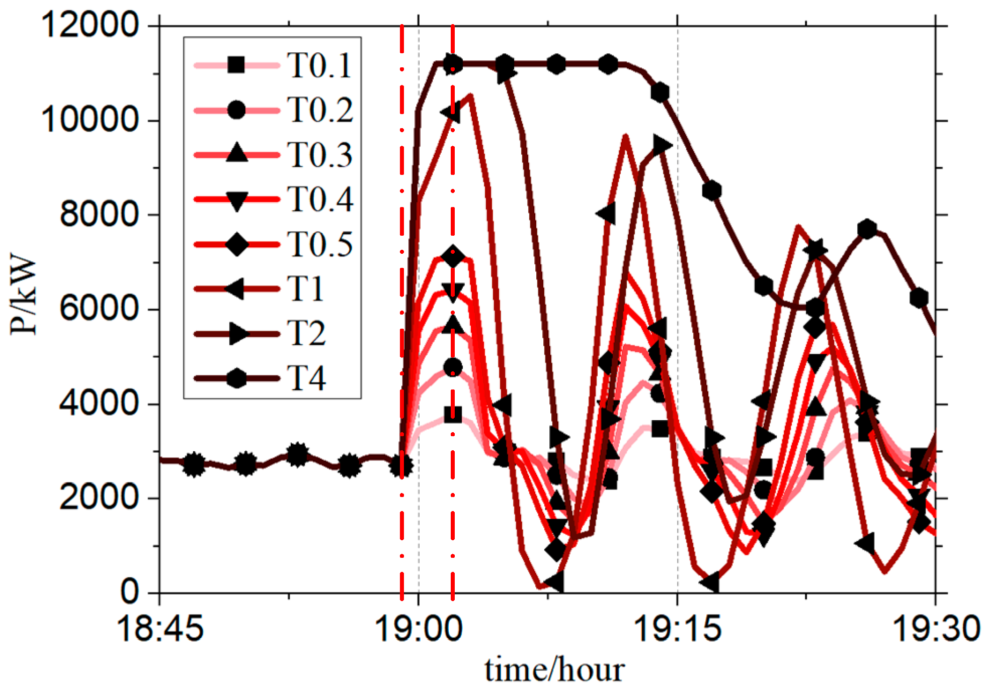
The relationship between the instantaneous power and the change in the setpoint temperature is shown in Figure 7.
It is observed that in the heating mode, an increase in the setpoint temperature of the aggregate will cause an increase in the load. The range of values of the load limit of the virtual house model can be obtained using the relationship shown in Figure 7. Figure 8 shows that the load rebound of the aggregated unit contains the detailed models of 2000 air conditioning systems created in Gridlab-D; an increase in the temperature settings at a given moment can be determined. The rebound peak load shown in Figure 8 is in agreement with the relationship shown in Figure 7. However, the rebound peak load does not occur at the moment of changing the setpoint temperature; there is a short period of increase (shown as the red dotted line in Figure 8) because of the cycle time of the air conditioning compressor. This occurs because the compressor requires some time to return to the running state from the pause state. This time is called the cycle time.
In this case, the initial temperature of the equivalent house can also be calculated using the law of energy conservation.
4. Load Control Scheme
The proposed load control scheme is divided into two stages, i.e., the load reduction stage and temperature recovery stage. The purpose of the load reduction stage is to achieve load control and the purpose of the temperature recovery stage is to restore the room temperature while suppressing the load rebound and oscillation.
In the load reduction stage, depending on the requirements of the load reduction, the average indoor temperature at the end of load reduction is first calculated by the aggregate model. Then the rate of decrease in the average temperature can be calculated. The rate of decrease will be broadcasted to all TCAs. Finally, according to the minimum control time (△t), the set temperature difference (△T) before and after can be calculated and implemented. Figure 9 shows the DR process of an air conditioning system. The green background represents the load reduction state. As shown in the figure, as the set temperature decreases, the time required for the temperature to increase in each heating cycle of the air conditioner decreases. In addition, it takes longer for the indoor temperature to decrease; therefore, the air conditioning power decreases at the load reduction stage. The load can be controlled by setting the value △T based on the aggregate model.
In the temperature recovery stage, the total load required to restore all the air conditioning systems to their original room temperature can be calculated by the aggregate model. Then, according to the rebound load limit value, the minimum time required (Tmin) to exit the DR can be obtained. Subsequently, the set temperature of the air conditioner can be calculated by Equation (14). is heterogeneous because the minimum control time (△t) is different in each air conditioner. As shown in Figure 9, the red background represents the temperature recovery state.
The control diagram is shown in Figure 10. We monitor the indoor temperature and total load and when the values exceed the alarm values, we repeat the process. The proposed DR scheme achieves load control using infrequent communications and few control signals, whereas the queuing method requires frequent communication with and control of each air conditioner; the higher the requirement for load control accuracy, the stricter the demand for communication and control is.
5. Results and Discussion
To verify the applicability of the proposed aggregate model and the effectiveness of the DR scheme, models of 2000 air conditioning units are created in Gridlab-D. These air conditioning units are in the heating mode when the outdoor temperature is set to 10 °C.
Three scenarios are simulated and discussed, namely the homogeneous model and the heterogeneous model. In the third model, each air conditioning unit has a different setpoint temperature based on the heterogeneous model. The detailed models are created in Gridlab-D and the virtual house is created by the proposed aggregate method. The aggregated system receives a DR command that reduces the load by 50 percent from 18:30 to 19:00. The time period for exiting the DR is 19:00 to 20:00. The parameters of the virtual house are solved by the proposed aggregate model.
The specific parameters of the three scenarios are shown in Table 3. The first scenario represents the homogeneous model, in which the aggregated area of the houses is 185.8 m2. The second scenario represents the heterogeneous model with the same setpoint temperature; the aggregated area of the houses meets a uniform distribution and is 167–204 m2. The third scenario represents the heterogeneous model with the different setpoint temperatures; the aggregated area of the houses also meets the uniform distribution and is 167–204 m2. The initial setpoint temperature of the aggregated houses meets the uniform distribution at 23.3–24.4 °C. The average temperature is calculated for the virtual house model and broadcast to each air conditioning unit at a time interval of 5 min. The load-average temperature curve of the aggregated units under a DR scheme is shown in Figure 11; (a) represents the first scenario, (b) represents the second scenario, (c) represents the third scenario, and (d) represents the queuing method. Figure 12 shows the indoor temperature curves of 200 units randomly selected from the aggregated unit.
It can be seen in Figure 11a that the total load quickly decreased to 50% and the load was maintained for half an hour; the average temperature of the aggregate unit fell by more than 0.5 degree centigrade. Compared with Figure 11a, a load rebound is observed at 20:00 in Figure 11b because the proposed virtual house model has an error for heterogeneous houses. As can be seen from Figure 11c, different setpoint temperatures do not affect the load control but suppress the load rebound. In Figure 11d, the air conditioning units are divided into 10 groups for queuing and the performance of the load control accuracy or load oscillation suppression is lower than for the proposed DR scheme.
Figure 12 shows the load curve of the aggregated under the DR schemes. It is evident that the proposed DR scheme exhibits a good load control for the heterogeneous model and the homogeneous model. For a large number of heterogeneous models, the proposed aggregate model is applicable and achieves accurate load control and suppression of load rebound.
As shown in Figure 13, the proposed DR scheme not only reflects the equality of consumers by being able to participate in the DR (unlike in Figure 13d, each consumer in Figure 13a, Figure 13b, and Figure 13c participates in the load control) but also retains the different temperature settings of the consumers (in Figure 13c, consumers with different temperature settings retain their temperature setting preferences).
6. Conclusions
In this paper, an aggregate model for air conditioning loads and their DR control strategy has been proposed. To validate the aggregate model, a detailed model of 2000 air conditioners was established in Gridlab-D to conduct comparisons. The simulation results showed that the temperature error between the aggregate model and the detailed model was comparatively low and its influence on the load control was negligible. Furthermore, the aggregate model does not require user information and it is easy to implement. In addition, the DR scheme based on the aggregate model is less dependent on communication infrastructure. The proposed DR scheme was verified using the detailed model and the results showed that the proposed scheme achieved accurate load control. In addition, the DR scheme also guarantees the different temperature settings by different users so that the comfort level of the users is not affected when implementing the DR. In a future study, we will improve the aggregate model and eliminate the temperature calculation error.
Author Contributions
Conceptualization, X.Z. and J.S.; methodology, X.Z.; software, X.Z.; validation, Y.T.; formal analysis, Y.L.; investigation, S.L.; resources, K.G.; data curation, X.Z.; writing—original draft preparation, X.Z.; writing—review and editing, X.Z.; visualization, X.Z.; supervision, J.S.
Funding
This research was funded by the Science and Technology Project of SGCC under Grant 52150018000N.
Conflicts of Interest
The authors declare no conflict of interest.
Nomenclature
| TCLs | Thermostatically controlled loads |
| DR | Demand response |
| ETP | Equivalent thermal parameters |
| PDE | Partial differential equation |
| Air heat capacity (Btu/°C) | |
| Mass (of the building and its content) heat capacity (Btu/°C) | |
| The gain/heat loss coefficient (Btu/°C*h) to the ambient air | |
| The gain/heat loss coefficient (Btu/°C*h) between air and mass | |
| Air temperature inside the house (°C) | |
| Mass temperature inside the house (°C) | |
| Outdoor temperature (°C) | |
| Set temperature of air conditioning | |
| Deadband of air conditioning | |
| Heat gain from air node (Btu) | |
| Heat gain from mass node (Btu) | |
| Heat gain from solar (Btu) | |
| Heat gain from HVAC (Btu) | |
| Heat gain from internal gains (Btu) | |
| A | Floor area (m2) |
| Awt | The gross exterior wall area (m2) |
| Ag | The gross window area (m2) |
| Ad | The total door area (m2) |
| Aw | The net exterior wall area (m2) |
| Ac | The net exterior ceiling area (m2) |
| Af | The net exterior floor area (m2) |
| R | Floor aspect ratio |
| Rw | R-value, walls |
| Rc | R-value, ceilings |
| Rf | R-value, floors |
| Rd | R-value, doors |
| hs | Interior surface heat transfer coefficient |
| mf | Total thermal mass per unit floor area (m2) |
| h | Ceiling height (m) |
| I | Infiltration volumetric air exchange rate |
| n | Total number of air conditioners |
| The difference between the indoor temperature and the set temperature (°C) | |
| (ECR) | Exterior ceiling, fraction of total |
| (EFR) | Exterior floor, fraction of total |
| (EWR) | Exterior wall, fraction of total |
| (WWR) | Window/exterior wall area ratio |
References
- U. S. Department of Energy. Benefits of Demand Response in Electricity Markets and Recommendations for Achieving Them; A Report to the United States Congress Pursuant to Section 1252 of the Energy Policy Act of 2005; U. S. Department of Energy: Washington, DC, USA, 2006.
- Torriti, J.; Hassan, M.G.; Leach, M. Demand response experience in Europe: Policies, programmes and implementation. Energy 2010, 35, 1575–1583. [Google Scholar] [CrossRef] [Green Version]
- Muratori, M.; Rizzoni, G. Residential Demand Response: Dynamic Energy Management and Time-Varying Electricity Pricing. IEEE Trans. Power Syst. 2016, 31, 1108–1117. [Google Scholar] [CrossRef]
- Lu, N.; Chassin, D.P. A state-queueing model of thermostatically controlled appliances. IEEE Trans. Power Syst. 2004, 19, 1666–1673. [Google Scholar] [CrossRef]
- Manichaikul, Y.; Schweppe, F.C. Physically based industrial electric load. IEEE Trans. Power Apparatus Syst. 1979, 98, 1439–1445. [Google Scholar] [CrossRef]
- Sanandaji, B.M.; Hao, H.; Poolla, K. Fast regulation service provision via aggregation of thermostatically controlled loads. In Proceedings of the 2014 47th Hawaii International Conference on System Sciences, Waikoloa, HI, USA, 6–9 January 2014; pp. 2388–2397. [Google Scholar]
- Bashash, S.; Fathy, H.K. Modeling and control of aggregate air conditioning loads for robust renewable power management. IEEE Trans. Control Syst. Technol. 2013, 21, 1318–1327. [Google Scholar] [CrossRef]
- Zhao, L.; Zhang, W. A unified stochastic hybrid system approach to aggregated load modeling for demand response. In Proceedings of the 2015 54th IEEE Conference on Decision and Control (CDC), Osaka, Japan, 15–18 December 2015; pp. 6668–6673. [Google Scholar]
- Mathieu, J.; Koch, S.; Callaway, D. State estimation and control of electric loads to manage real-time energy imbalance. IEEE Trans. Power Syst. 2013, 28, 430–440. [Google Scholar] [CrossRef]
- Zhang, W.; Kalsi, K.; Fuller, J.; Elizondo, M.; Chassin, D. Aggregate model for heterogeneous thermostatically controlled loads with demand response. In Proceedings of the 2012 IEEE Power and Energy Society General Meeting, San Diego, CA, USA, 22–26 July 2012; pp. 1–8. [Google Scholar]
- Lu, N.; Chassin, D.P.; Widergren, S.E. Modeling uncertainties in aggregated thermostatically controlled loads using a state queueing model. IEEE Trans. Power Syst. 2005, 20, 725–733. [Google Scholar] [CrossRef]
- Callaway, D.S. Tapping the energy storage potential in electric loads to deliver load following and regulation, with application to wind energy. Energy Convers. Manag. 2009, 50, 1389–1400. [Google Scholar] [CrossRef]
- Lu, N.; Zhang, Y. Design considerations of a centralized load controller using thermostatically controlled appliances for continuous regulation reserves. IEEE Trans. Smart Grid 2013, 4, 914–921. [Google Scholar] [CrossRef]
- Tindemans, S.H.; Trovato, V.; Strbac, G. Decentralized control of thermostatic loads for flexible demand response. IEEE Trans. Control Syst. Technol. 2015, 23, 1685–1700. [Google Scholar] [CrossRef]
- Erdinç, O.; Taşcıkaraoğlu, A.; Paterakis, N.G.; Eren, Y.; Catalão, J.P.S. End-User Comfort Oriented Day-Ahead Planning for Responsive Residential HVAC Demand Aggregation Considering Weather Forecasts. IEEE Trans. Smart Grid 2017, 8, 362–372. [Google Scholar] [CrossRef]
- Hu, J.; Cao, J.; Chen, M.Z.; Yu, J.; Yao, J.; Yang, S.; Yong, T. Load Following of Multiple Heterogeneous TCL Aggregators by Centralized Control. IEEE Trans. Power Syst. 2017, 32, 3157–3167. [Google Scholar] [CrossRef]
- Ihara, S.; Schweppe, F.C. Physically Based Modeling of Cold Load Pickup. IEEE Trans. Power Appar. Syst. 1981, PAS-100, 4142–4150. [Google Scholar] [CrossRef]
- Mortensen, R.E.; Haggerty, K.P. A stochastic computer model for heating and cooling loads. IEEE Trans. Power Syst. 1988, 3, 1213–1219. [Google Scholar] [CrossRef]
- Banash, S.; Fathy, H. Modeling and Control Insights into Demandside Energy Management through Setpoint Control of Thermostatic Loads. In Proceedings of the 2011 American Control Conference, San Francisco, CA, USA, 29 June–1 July 2011. [Google Scholar]
- Sonderegger, R.C. Dynamic Models of House Heating based on Equivalent Thermal Parameters. Bachelor’s Ph.D. Thesis, Princeton University, Princeton, NJ, USA, 1978. [Google Scholar]
- Hao, H.; Sanandaji, B.; Poolla, K.; Vincent, T. Aggregate flexibility of thermostatically controlled loads. IEEE Trans. Power Syst. 2015, 30, 189–198. [Google Scholar] [CrossRef]
- Koch, S.; Mathieu, J.L.; Callaway, D.S. Modeling and Control of Aggregated Heterogeneous Thermostatically Controlled Loads for Ancillary Services. In Proceedings of the 17th Power system Computation Conference, Stockholm, Sweden, 22–26 August 2011. [Google Scholar]
Figure 1.
ETP representation of the heat flow in typical residences

Figure 2.
Equivalent thermal parameters circuit

Figure 3.
The virtual house as an aggregation of two houses.

Figure 4.
The average indoor temperature difference. (a) Temperature differences from 0 to 5 h; (b) temperature differences from 0 to 30 min.
Figure 4.
The average indoor temperature difference. (a) Temperature differences from 0 to 5 h; (b) temperature differences from 0 to 30 min.

Figure 5.
The aggregated responses of 2000 homogeneous and heterogeneous TCLs.

Figure 6.
Indoor air temperature for a single air conditioning system.

Figure 7.
The relationship between instantaneous power and the change in the setpoint temperature.

Figure 8.
The load rebound of the aggregate model.

Figure 9.
The demand response process of an air conditioning system.

Figure 10.
The proposed aggregated load control scheme.

Figure 11.
The load-average temperature curve of the aggregation under the demand response scheme. (a) represents the first scenario, (b) represents the second scenario, (c) represents the third scenario, and (d) represents the queuing method.
Figure 11.
The load-average temperature curve of the aggregation under the demand response scheme. (a) represents the first scenario, (b) represents the second scenario, (c) represents the third scenario, and (d) represents the queuing method.


Figure 12.
The load curve of the aggregated units under the demand response scheme.

Figure 13.
The indoor temperature curves of 200 units randomly selected from the aggregated units; (a) represents the first scenario, (b) represents the second scenario, (c) represents the third scenario, and (d) represents the queuing method.
Figure 13.
The indoor temperature curves of 200 units randomly selected from the aggregated units; (a) represents the first scenario, (b) represents the second scenario, (c) represents the third scenario, and (d) represents the queuing method.


Table 1.
Relationship between the house structure and area
| Symbol | Calculation |
|---|---|
Table 2.
Area distributions (U represents normal distribution, N repersents uniform distribution).
| Number | Area Distributions (sf2) | Area Distributions (m2) |
|---|---|---|
| 1 | U(1800,2200) | U(167,204) |
| 2 | U(1600,2400) | U(149,223) |
| 3 | U(1400,2600) | U(130,242) |
| 4 | U(1200,2800) | U(111,260) |
| 5 | U(1000,3000) | U(93,279) |
| 6 | N(2000,1002) | N(186,9.32) |
| 7 | N(2000,2002) | N(186,18.62) |
| 8 | N(2000,4002) | N(186,37.22) |
| 9 | U(1400,1600) and U(2400,2600) | U(130,149)and U(223,242) |
| 10 | U(1000,1200) and U(2800,3000) | U(93,111) and U(260,279) |
| 11 | U(800,1200) and U(2600,3400) | U(74,111) and U(242,316) |
| 12 | U(800,1200) and U(3800,4200) | U(74,111) and U(353,390) |
Table 3.
The specific parameters of the three scenarios.
| Label | Area () | Area () | Initial Setpoint (°F) | Initial Setpoint (°C) | Demand Response Scheme |
|---|---|---|---|---|---|
| Scenario (a) | 2000 | 185.8 | 75 | 23.8 | Proposed method |
| Scenario (b) | U(1800–2200) | U(167–204) | 75 | 23.8 | Proposed method |
| Scenario (c) | U(1800–2200) | U(167–204) | 74–76 | 23.3–24.4 | Proposed method |
| Scenario (d) | 2000 | 185.8 | 75 | 23.8 | Queuing method |
© 2019 by the authors. Licensee MDPI, Basel, Switzerland. This article is an open access article distributed under the terms and conditions of the Creative Commons Attribution (CC BY) license (http://creativecommons.org/licenses/by/4.0/).
Share and Cite
MDPI and ACS Style
Zhou, X.; Shi, J.; Tang, Y.; Li, Y.; Li, S.; Gong, K. Aggregate Control Strategy for Thermostatically Controlled Loads with Demand Response. Energies 2019, 12, 683. https://doi.org/10.3390/en12040683
AMA Style
Zhou X, Shi J, Tang Y, Li Y, Li S, Gong K. Aggregate Control Strategy for Thermostatically Controlled Loads with Demand Response. Energies. 2019; 12(4):683. https://doi.org/10.3390/en12040683
Chicago/Turabian StyleZhou, Xiao, Jing Shi, Yuejin Tang, Yuanyuan Li, Shujian Li, and Kang Gong. 2019. "Aggregate Control Strategy for Thermostatically Controlled Loads with Demand Response" Energies 12, no. 4: 683. https://doi.org/10.3390/en12040683
Note that from the first issue of 2016, this journal uses article numbers instead of page numbers. See further details here.