Wind Power Prediction Based on Extreme Learning Machine with Kernel Mean p-Power Error Loss

Abstract

In recent years, more and more attention has been paid to wind energy throughout the world as a kind of clean and renewable energy. Due to doubts concerning wind power and the influence of natural factors such as weather, unpredictability, and the risk of system operation increase, wind power seems less reliable than traditional power generation. An accurate and reliable prediction of wind power would enable a power dispatching department to appropriately adjust the scheduling plan in advance according to the changes in wind power, ensure the power quality, reduce the standby capacity of the system, reduce the operation cost of the power system, reduce the adverse impact of wind power generation on the power grid, and improve the power system stability as well as generation adequacy. The traditional back propagation (BP) neural network requires a manual setting of a large number of parameters, and the extreme learning machine (ELM) algorithm simplifies the time complexity and does not need a manual setting of parameters, but the loss function in ELM based on second-order statistics is not the best solution when dealing with nonlinear and non-Gaussian data. For the above problems, this paper proposes a novel wind power prediction method based on ELM with kernel mean p-power error loss, which can achieve lower prediction error compared with the traditional BP neural network. In addition, to reduce the computational problems caused by the large amount of data, principal component analysis (PCA) was adopted to eliminate some redundant data components, and finally the efficiency was improved without any loss in accuracy. Experiments using the real data were performed to verify the performance of the proposed method.

1. Introduction

In view of the increasing depletion of fossil fuels and the environmental pollution caused by them, every country is sparing no effort to develop technologies for renewable energy power generation. Because of the large development potential strengths of wind energy, using wind power to generate electricity has obtained the support of the vast majority of countries, thus undergoing rapid development [1,2,3]. As opposed to more conventional power sources, wind power is highly random, intermittent, unstable, and inflexible, due to the influence of meteorological conditions and surrounding terrain environment. Moreover, wind farms are typically located in remote areas at the end of a power system, where grids are relatively weak. In order to ensure the stable operation of the power grid and the reliability of the power supply system, the latter needs to be planned effectively [4]. In order to cope with the randomness, intermittency, instability and inflexibility of wind power, the system must increase the reserve capacity of its power supply system in operation to ensure the normal power supply to users when the wind power output is insufficient [5,6]. However, the increase of reserve capacity indirectly increases the overall cost of wind power operation, so it is necessary to predict the output power of large wind farms. Therefore, wind power prediction systems have become an indispensable part of the practical application of wind power. Through the accurate prediction of wind power generation in the short and medium term, the remote reserve capacity of the power grid can be significantly reduced, which can effectively reduce the cost of wind power generation [7] and provide a reliable basis for the operation and dispatch of the power grid, so as to ensure the safe and stable operation of the power system [8,9,10].

Wind power is affected by many factors, including wind speed, temperature, pressure, humidity, altitude, latitude, and so on. These factors are also correlated with each other, which leads to the strong randomness of wind power that makes the prediction more and more difficult to obtain a satisfactory accuracy. There are many methods used for predicting wind speed. A simple traditional method is the continuous prediction method, which uses the wind power of the nearest point to forecast the predicted value of the next point [11]. The Kalman filtering method combines wind speed and power as state variables to establish a spatial model for prediction [12,13]. The time series method uses a large amount of historical data through model identification, parameter estimation, and model tests to determine a mathematical model that can describe the time series studied, which then deduces the prediction model. At present, the most commonly used model is the auto-regressive and moving average [14,15]. An artificial neural network method can also be applied to wind power prediction, having the ability to self-learn, self-organize, and self-adapt. The most widely applied method is the back-propagation (BP) neural network [16,17,18,19]. Other methods include fuzzy logic, and spatial correlation [20,21]. The literature [22] uses a variety of machine learning technologies to predict wind power and is divided into two steps [23]. First, relevant data are used for wind power prediction, and then the predicted value is smoothed. The literature [24] proposes a new neural network model, recursive variational model decomposition- long short-term memory (R-VMD-LSTM) and direct VMD-LSTMD, for wind power prediction.

Among the above prediction methods, the neural network method has been widely used in recent years because of its high accuracy and strong adaptive ability. A BP neural network is suitable for solving non-linear problems [25], but it also has some drawbacks, such as slow convergence speed, long processing times, easy-to-fall-into local minimum points, and the need to determine the number of intermediate layers and middle layer nodes based on experience (e.g., a large number of network training parameters need to be manually set). In recent years, the extreme learning machine (ELM) of the single-layer neural network model was proposed by professor Huang [26,27]. It only needs to set the number of hidden nodes in the network and does not need to set the input weight matrix of the network nor the deviation of hidden elements. It has a fast learning speed and good generalization performance, and has been widely applied for time series prediction [28], short-term load forecasting [29], wind power ramp events prediction [30], and much more [31,32,33,34]. In solving the weight matrix, the ELM adopts the least square method. If the non-linear and non-Gaussian degree of data is too large [35], the traditional loss function optimization is not a good solution. In order to solve this problem, Huber’s min-max loss [36], risk-sensitive loss [37], correntropy loss [38,39,40], and mean p-power error (MPE) loss [41] appear in machine learning. At present, a novel loss function called kernel mean p-power error (KMPE), was developed by Chen [42], which can be viewed as the MPE loss in kernel space; it has been applied to machine learning. The KMPE as a loss function has been applied to the ELM to enhance its performance when the data includes non-Gaussian characteristics.

Based on previous work, this paper proposes a new wind power prediction method, which not only improves the accuracy, but also improves the complexity of the algorithm. The main contributions of this paper are summarized as follows:

• Taking into account the non-linear and non-Gaussian characteristics of the wind power data [19,43], a novel wind power prediction scheme was developed, using the ELM with KMPE loss, and the prediction accuracy was significantly improved by taking advantage of the novel method. Furthermore, the novel prediction method mainly uses the ELM model, which can solve the problem that the BP neural network needs to set a large number of parameters artificially.
• In addition, considering the excessive influence factors of wind power which may lead to higher computational complex, this paper adopts the principal component analysis (PCA) [44,45] to reduce the redundant components and only get the components with high correlation with wind power, in order to facilitate the algorithm efficiency.

The rest of this paper is organized as follows. Section 2 gives a brief review of Extreme Learning Machine with Kernel Mean p-Power Error Loss (ELM-KMPE). Section 3 proposes the wind power prediction scheme based on ELM-KMPE with PCA. The proposed prediction method is validated by using real data in Section 4. Finally, Section 5 concludes with a summary of the main contributions and provides future research directions.

2. Brief Review of ELM-KMPE

2.1. Brief Review of ELM

2.1.1. Review of the ELM

An ELM is a fast Single-hidden Layer Feedforward Neural (SLFN) training algorithm. The characteristic of this algorithm is that in the process of determining network parameters, hidden layer node parameters are selected randomly, with no adjustments needed in the training process. The only optimal solution can be obtained by setting the number of neurons in the hidden layer. The external weight of the network is the least square solution obtained by minimizing the square loss function (ultimately converted into the Moore–Penrose generalized inverse problem for solving a matrix). In this way, no iterative steps are needed in the determination process of network parameters, thus greatly reducing the adjustment time of network parameters. Compared with the traditional training method (BP neural network), this method has a fast learning speed and a good generalization performance.

For a single hidden layer neural network, the structure is shown in Figure 1. Suppose there are N training samples (x_j, t_j), where,

$$X_j={[x_{j1},x_{j2},\dots ,x_{jn}]}^T\in R^n$$

(1)

$$t_j={[t_{j1},t_{j2},\dots ,t_{jm}]}^T\in R^m$$

(2)

For L hidden layer neuron networks, the expected output is shown below according to the weight matrix and threshold value

$${\displaystyle \sum _{i=1}^L{\beta }_{i}g}(W_i\cdot X_j+b_i)=o_j,j=1,2,\dots ,N$$

(3)

$$g(x)=\frac{1}{1+\exp (x)}$$

(4)

Among them, the g(x) as the activation function, W_i = [w_i1, w_i2, …, w_in]^T is i input weights of hidden layer units, b_i is the ith bias of hidden layer units, β_i = [i₁,i₂,…, i_m]^T is the i output of the hidden layer unit weight , o_j is the expected output, and W_i·X_j represents the inner product of W_i and X_j.

2.1.2. ELM Learning Goals

The learning objective is to make the distance between the expected output and the actual sample output as close as possible to 0, as shown in Equation (5) below

$${\displaystyle \sum _{j=1}^N\Vert o_j-t_j\Vert }=0$$

(5)

In combination with Equations (3) and (5), there are W_i, X_j and b_i

$${\displaystyle \sum _{i=1}^L{\beta }_{i}g}(W_i\cdot X_j+b_i)=t_j,j=1,2,\dots ,N$$

(6)

Equation (6) is expressed as matrix

$$H\cdot \beta =T$$

(7)

where H denotes the output of the hidden layer node, β is the output weight, and T stands for the expected output. Here is an example of an H neural network:

$$H(a_1,\dots ,a_L;b_1,\dots ,b_L;x_1,\dots x_L)={\left[\begin{array}{l}G(a_1,b_1,x_1)\hspace{0.17em}\hspace{0.17em}\cdots \hspace{0.17em}\hspace{0.17em}G(a_L,b_L,x_1)\\ \hspace{0.17em}\hspace{0.17em}\hspace{0.17em}\hspace{0.17em}\hspace{0.17em}\hspace{0.17em}\hspace{0.17em}\hspace{0.17em}\hspace{0.17em}⋮\hspace{0.17em}\hspace{0.17em}\hspace{0.17em}\hspace{0.17em}\hspace{0.17em}\hspace{0.17em}\hspace{0.17em}\hspace{0.17em}\hspace{0.17em}\ddots \hspace{0.17em}\hspace{0.17em}\hspace{0.17em}\hspace{0.17em}\hspace{0.17em}\hspace{0.17em}\hspace{0.17em}\hspace{0.17em}\hspace{0.17em}\hspace{0.17em}\hspace{0.17em}⋮\\ G(a_1,b_1,x_N)\hspace{0.17em}\cdots \hspace{0.17em}\hspace{0.17em}G(a_L,b_L,x_N)\end{array}\right]}_{N\times L}$$

(8)

$$\beta ={\left[\begin{array}{l}{\beta }_1^T\\ \hspace{0.17em}\hspace{0.17em}⋮\\ {\beta }_L^T\end{array}\right]}_{L\times d}\hspace{0.17em}\hspace{0.17em}\hspace{0.17em}\hspace{0.17em}\hspace{0.17em}T={\left[\begin{array}{l}{t}_1^T\\ \hspace{0.17em}⋮\\ t_1^T\end{array}\right]}_{N\times m}$$

(9)

In order to be able to train a single hidden layer neural network, we hope to get ${\widehat{W}}_i$, ${\widehat{b}}_i$ and ${\beta }_i$, so that

$$\hspace{0.17em}\hspace{0.17em}\hspace{0.17em}\hspace{0.17em}\Vert H({\widehat{W}}_i,{\widehat{b}}_i)\cdot \widehat{\beta }-T\Vert ={\min }_{W,b,\beta }\Vert H(W_i,b_i)\cdot \beta -T\Vert$$

(10)

where i = 1,2, …, L, so that the minimum loss function is

$$E={{\displaystyle \sum _{j=1}^N\Vert {\displaystyle \sum _{i=1}^L{\beta }_i\cdot g(W_i\cdot X_j+b_i)-t_j}\Vert }}^2$$

(11)

2.1.3. ELM Learning Methods

In machine learning, the gradient descent method is often used for optimization, but all parameters of the gradient descent method are uniquely determined in the process of iteration. Once the weight matrix W_i and the deviation vector b_i of the hidden layer are determined, there will be the corresponding output matrix H. All single hidden layer neural networks can be transformed into a linear system: H·β = T. At this point, the output weight vector is as follows

$$\widehat{\beta }=H^{+}\cdot T$$

(12)

where H⁺ is the generalized Moore–Penrose inverse matrix of H. If L is used to represent the number of neurons in the hidden layer and N is used to represent the number of training samples, then the matrix H is square and invertible. However, L tends to be less than N, so generalized inverse matrices are generally used.

2.2. Review of the KMPE

Learning theory generally aims at minimizing the loss function. Traditional ELM minimizes the squared loss function to obtain the least squares solution, which minimizes the mean square error (MSE) between the expected output and the actual output. However, as a kind of second-order statistics, MSE is too sensitive to non-Gaussian data and nonlinear outliers, so it is not an optimal solution. In order to solve the above problems, reference [42] used the mean p-power error (MPE) loss to optimize it, and the appropriate p value could then be used to process Gaussian data with large outliers.

At present, a non-second-order measure in kernel space, called the kernel mean p-power error (KMPE), was developed: it is the MPE in kernel space and, naturally, the non-second-order measure in the original space. KMPE will be reduced to a C-loss at p = 2, but when used as a loss function in robust learning, the appropriate p value can be optimized for C-loss [42]. In this work, the KMPE is utilized as a loss function in ELM to develop a novel ELM model which can effectively address the non-linear and non-Gaussian data. Given two random variables X and Y, the KMPE [17] loss was defined in kernel space as

$$\begin{array}{ll}{C}_{p-loss}(X,Y)& =2^{-p/2}\mathrm{E}\left[\left|\right|\Phi (X)-\Phi (Y)|{|}_{\mathrm{H}}^p\right]\\ & =2^{-p/2}\mathrm{E}\left[{\left(\left|\right|\Phi (X)-\Phi (Y)|{|}_{\mathrm{H}}^2\right)}^{p/2}\right]\\ & =2^{-p/2}\mathrm{E}\left[{\left(2-2{\kappa }_{\sigma }\left(X-Y\right)\right)}^{p/2}\right]\\ & =\mathrm{E}\left[{\left(1-{\kappa }_{\sigma }\left(X-Y\right)\right)}^{p/2}\right]\end{array}$$

(13)

where p > 0 denotes the power parameter, E[.] denotes the expectation operator, $\Phi (x)$is a nonlinear mapping induced by a Mercer ${\kappa }_{\sigma }(x,\cdot )$, and${\langle \cdot ,\cdot \rangle }_H$represents the inner product in the kernel space H, satisfying ${\kappa }_{\sigma }\left(X-Y\right)={\langle \Phi (X),\Phi (Y)\rangle }_H$. In general, the Gaussian kernel is used as the kernel function as:

$$k(x,y)=k_{\sigma }(x-y)=\exp (-\frac{{(x-y)}^2}{2{\sigma }^2})$$

(14)

The KMPE will be equivalent to the C-loss when p = 2. In practice, only finite samples ${\{(x_i,y_i)\}}_{i=1}^N$ of the variables X and Y are given. Hence, we obtain the empirical KMPE loss as:

$${\widehat{C}}_{p-loss}(X,Y)=\frac{1}{N}{\displaystyle \sum _{i=1}^N{\left(1-{\kappa }_{\sigma }(x_i-y_i)\right)}^{p/2}}$$

(15)

The KMPE loss function for each sample can be represented as:

$$J_{C_{p-loss}}(e)={\left(1-{\kappa }_{\sigma }\left(e\right)\right)}^{p/2}$$

(16)

where e = x − y.

2.3. ELM Based on KMPE Loss

After having considered a wind power prediction error distribution to Gaussian distribution [19], based on the ELM before the minimum square error (MSE-) and prediction-based forecast, we now introduce the ELM algorithm based on KMPE loss [42].

The output equation of ELM with L hidden layer nodes is:

$$y_i={\displaystyle \sum _{j=1}^L{\beta }_{j}f(W_j\cdot X_i+b_j)}$$

(17)

The equation above is expressed in vector form:

$$Y=H\beta$$

(18)

The output weight vector offset can be solved by minimizing the loss of regularized MSE (or least squares):

$$J_{MSE}(\beta )={\displaystyle \sum _{i=1}^N{e}_i^2+\lambda {\left|\left|\beta \right|\right|}_2^2}={\left|\left|H\beta -T\right|\right|}_2^2+\lambda {\left|\left|\beta \right|\right|}_2^2$$

(19)

where e_i = t_i − y_i is the error of the ith target response and the ith actual output, respectively, and the value of λ >0 represents the regular coefficient to prevent over-fitting. T = (t₁, …, t_N)^T is the target response vector.

Through a pseudo-inversion operation, unique solutions can be easily obtained in case of loss.

$$\beta ={\left[H^{T}H+\lambda I\right]}^{-1}{H}^{T}T$$

(20)

KMPE expression is based on loss function:

$$\begin{array}{l}{J}_{KMPE}(\beta )={\widehat{C}}_p(T,H\beta )+\lambda {\left|\left|\beta \right|\right|}_2^2=\frac{1}{N}{\displaystyle \sum _{i=1}^N{(1-k_{\sigma }(e_i))}^{p/2}}+\lambda {\left|\left|\beta \right|\right|}_2^2\\ \hspace{0.17em}\hspace{0.17em}\hspace{0.17em}\hspace{0.17em}\hspace{0.17em}\hspace{0.17em}\hspace{0.17em}\hspace{0.17em}\hspace{0.17em}\hspace{0.17em}\hspace{0.17em}\hspace{0.17em}\hspace{0.17em}=\frac{1}{N}{\displaystyle \sum _{i=1}^N{(1-\exp (-\frac{e_i^2}{2{\sigma }^2}))}^{p/2}}+\lambda {\left|\left|\beta \right|\right|}_2^2\end{array}$$

(21)

Then, we compute the gradient of Equation (21) and set it to zero yields

$$\begin{array}{l}\frac{\partial }{\partial \beta }{J}_{KMPE}(\beta )=0\\ \Rightarrow \frac{1}{N}{\displaystyle \sum _{i=1}^N\left[\frac{-p}{2{\sigma }^2}{(1-k_{\sigma }(e_i))}^{\frac{p-2}{2}}{k}_{\sigma }(e_i)e_i{h}_i^T\right]+2\lambda \beta }=0\\ \Rightarrow {\displaystyle \sum _{i=1}^N\left[-{(1-k_{\sigma }(e_i))}^{\frac{p-2}{2}}{k}_{\sigma }(e_i)e_i{h}_i^T\right]+\frac{4{\sigma }^{2}N\lambda }{p}\beta }=0\\ \Rightarrow {\displaystyle \sum _{i=1}^N(\phi (e_i)h_i^T{h}_i\beta -\phi (e_i)t_i{h}_i^T)+{\lambda }^{\prime }\beta }=0\\ \Rightarrow {\displaystyle \sum _{i=1}^N(\phi (e_i)h_i^T{h}_i\beta )+{\lambda }^{\prime }\beta }={\displaystyle \sum _{i=1}^N\phi (e_i)t_i{h}_i^T}\\ \Rightarrow \beta ={\left[H^T\Lambda H+{\lambda }^{\prime }I\right]}^{-1}{H}^T\Lambda T\end{array}$$

(22)

where ${\lambda }^{\prime }=\frac{4{\sigma }^{2}N}{p}\lambda$ is the ith row of H matrix, $\phi (e_i)={(1-k_{\sigma }(e_i))}^{\frac{p-2}{2}}{k}_{\sigma }(e_i)$, and the Λ is a diagonal matrix, the diagonal elements ${\Lambda }_{ii}=\phi (e_i)$.

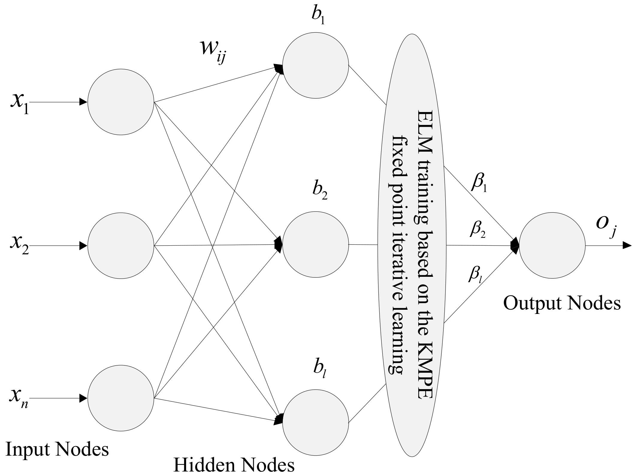
It is worked out that the optimal solution of $\beta ={\left[H^T\Lambda H+{\lambda }^{\prime }I\right]}^{-1}{H}^T\Lambda T$ is not a closed form solution, based on the right side of the matrix Λ on vector β, and β is by e_i = t_i − h_i β. It is actually a non-moving equation. Therefore, the real optimal solution can be used fixed-point iteration algorithm. The ELM-KMPE network structure optimization process using KMPE fixed point iteration which can be seen in Figure 2. In this paper, ELM-KMPE is proposed to be used for wind power prediction, which is significantly more accurate than the traditional ELM and verified by experiments.

Iterative Algorithm ELM-KMPE

The input samples: ${\left\{x_i,t_i\right\}}_{i=1}^N$

Output weight vector: β

Parameter Settings: number of hidden layer nodes L, regular factor lambda λ′, maximum iterative number M, width of nuclear σ, power parameter p and eventually tolerance ε.

Initialization: set β₀ = 0 and randomly initialize parameters W_j and b_j (j = 1, 2, …, L).

Step 1. From k = 1, 2, ..., M cycle.

Step 2. Calculate the error based on ${\beta }_{k-1}:e_i=t_i-h_i{\beta }_{k-1}$.

Step 3. Calculate diagonal matrix $\Lambda :{\Lambda }_{ii}=\phi (e_i)$.

Step 4. Update weight vector $\beta :{\beta }_k={[H^T\Lambda H+{\lambda }^{\prime }I]}^{-1}{H}^T\Lambda T$

Step 5. Until $\left|J_{KMPE}({\beta }_k)-J_{KMPE}({\beta }_{k-1})\right|<\epsilon$.

Step 6. End.

3. Wind Power Prediction Based on ELM-KMPE with Principal Component Analysis

3.1. Review of the PCA

The principal component analysis (PCA) [44,45] is a multivariate statistical analysis technique combining data compression and feature extraction. It seeks for multiple related variables to be replaced by several unrelated variables, which contain most information of the original variables. The data information is represented by the variance of the original variable. The larger the amount of information, the larger the variance. The total amount of information is generally represented by the accumulative variance contribution rate. The algorithm of the principal component analysis is made to obtain the eigenvalues of the data matrix of the input variable, sum up the variance corresponding to each input variable, and then determine the principal component according to the accumulated numerical value. The PCA method has been applied in a long short-term memory model for a prediction of wind turbine–grid interaction [46].

Here is a sample observation data matrix:

$$X=\left[\begin{array}{cccc}{x}_{11}& x_{12}& \cdots & x_{1p}\\ x_{21}& x_{22}& \cdots & x_{2p}\\ ⋮& ⋮& ⋮& ⋮\\ x_{n1}& x_{n2}& \cdots & x_{np}\end{array}\right]$$

(23)

For n observation data, each observation data has p variables, that is, p independent variables.

Step 1. The raw data is standardized

$$\hspace{0.17em}\hspace{0.17em}\hspace{0.17em}\hspace{0.17em}\hspace{0.17em}\hspace{0.17em}\hspace{0.17em}{x}_{ij}^{*}=\frac{x_{ij}-{\overline{x}}_j}{\sqrt{\mathrm{var}(x_j)}}\hspace{0.17em}\hspace{0.17em}\hspace{0.17em}\hspace{0.17em}\hspace{0.17em}\hspace{0.17em}\hspace{0.17em}(i=1,2,\cdots ,n;j=1,2,\cdots p)$$

(24)

Among them,

$${\overline{x}}_j=\frac{1}{n}{\displaystyle \sum _{i=1}^n{x}_{ij}}$$

(25)

$$\mathrm{var}(x_j)=\frac{1}{n-1}{\displaystyle \sum _{i=1}^n{(x_{ij}-{\overline{x}}_j)}^2}\hspace{0.17em}\hspace{0.17em}\hspace{0.17em}\hspace{0.17em}(j=1,2,\cdots ,p)$$

(26)

Step 2. The sample correlation coefficient matrix is calculated

$$R=Cov(X)=\left[\begin{array}{cccc}{r}_{11}& r_{12}& \cdots & r_{1p}\\ r_{21}& r_{22}& \cdots & r_{2p}\\ ⋮& ⋮& ⋮& ⋮\\ r_{p1}& r_{p2}& \cdots & r_{pp}\end{array}\right]$$

(27)

For convenience, we assume that the original data is still expressed after standardization, the correlation coefficient of the normalized data being:

$$r_{ij}=\frac{1}{n-1}{\displaystyle \sum _{t=1}^n{x}_{ti}{x}_{tj}}\hspace{0.17em}(i,j=1,2,\cdots ,p)$$

(28)

Step 3. The characteristic value (λ₁, λ₂, …, λ_p) of the correlation coefficient matrix R and the corresponding eigenvector a_i = (a_i1, a_i2, …, a_ip), i = 1,2, …, p using the Jacobian method.

Step 4. The contribution rate of principal component is calculated and the appropriate principal component is selected.

Principal component analysis can get the principal component, however, due to the diminishing variance of each principal component, it also decreases the amount of information. Thus, for the actual analysis, the general selection is not a main component; according to the size of the contribution rate of each principal component accumulated before selecting principal components, the contribution rate is a main component of variance accounted for the proportion of total variance, actually (e.g., a certain proportion of total eigenvalue combined). Namely,

$$\mathrm{Contribution}=\frac{{\lambda }_i}{{\displaystyle \sum _{i=1}^p{\lambda }_i}}$$

(29)

The higher the contribution rate, the stronger the information of the original variables contained in the principal component. The number of principal component K is mainly determined by the cumulative contribution rate of principal component; that is, the cumulative contribution rate is generally required to reach more than 85%, so as to ensure that the comprehensive variable can include most of the information of the original variable.

Step 5. According to the data of principal component score, further statistical analysis can be carried out.

3.2. The Prediction Scheme via the PCA

In general, various factors are used to predict the wind power, including wind speed, wind direction, air pressure, temperature and relative humidity. Among them, wind speed is affected by many factors, such as temperature, air pressure, topography, altitude, and latitude, so there are some redundant factors. When analyzing multivariate subjects, too many variables will increase the complexity of the subjects. We naturally want fewer variables and more information. There is often a certain correlation between different variables. When two variables are correlated and the correlation is relatively large, it is called redundancy. Therefore, we use the principal component analysis (PCA) to eliminate redundant repeated variables (closely related variables) for all previously proposed variables, and establish as few variables as possible, so that these new variables are pairwise irrelevant, and they can keep the original information as far as possible in reflecting the subject information. PCA is a combination of data compression and extraction methods of multivariate statistical analysis techniques; it seeks multiple related variables with several unrelated to replace, and the uncorrelated variables contains most of the original variable information.

Because the weight matrix of input variables in the ELM algorithm is generated randomly, input variables are processed immediately. Some scholars think that this treatment method is not reasonable and may affect the accuracy of the final output results, so we used the PCA method to preprocess of input variables and used the pretreatment results as an input variable to train the ELM model. After comparing the predicted results with previous results and further verifying the accuracy of the ELM, the algorithm complexity was reduced.

4. Experiment Results

4.1. Method Steps

This paper studied a power plant in China which has 30 wind turbines. The rated power of a single fan is 200 KW, and the rated power of the total generator is 6 MW.

In this paper, the historical data collected from the wind farm from 12:00 on 1 February 2013 to 12:00 on 2 February 2013 were taken as the main data for the verification of the following algorithms. The available historical data are mainly divided into two categories:

(1) NWP data: the numerical weather forecast, which mainly includes meteorological elements such as wind speed, wind direction, temperature, atmospheric humidity and atmospheric pressure.

For wind power plants without a Supervisory Control and Data Acquisition (SCADA) system installed, historical wind power data can be obtained from their internal energy management system, and the data of wind speed, wind direction, air temperature, humidity, and other influencing factors can be obtained through sensors installed on the wind measurement tower. In a wind farm where the terrain is less complex and the wind speed does not fluctuate significantly, a wind tower can reflect the wind speed of the entire wind farm. However, in the construction of wind power plants in steeper terrains, such as mountainous areas, it is necessary to set up several wind measuring towers to collect multiple values of wind speed for comprehensive consideration.

(2) The wind farm supervision and management and data acquisition (Supervisory Control and Data Acquisition) system automatically collects weather data at certain time intervals.

SCADA is a fully automated system integrating operation, adjusting and controlling automatically. At present, many wind farms in China and abroad use a SCADA system to collect data and process information, which enables a timely collection, processing, and monitoring of wind turbine data of wind farms, and enables a centralized management of all collected data. At the same time, the data can be monitored remotely by computer, and the system can be accessed at any time to see if there is any abnormality in the data.

This paper uses a short-term prediction method of learning as the wind power prediction method at intervals of 5 min. Using two sampling points and a wind farm SCADA system to automatically obtain related data, the wind power was measured: within the time of 1 day, the SCADA system took a total of 600 points, and in the process of dealing with this data, applied 500 of these points for the training of the model and the remaining 100 points for the detection of the model.

These data are generally non-linear, among which the wind speed distribution which had a generally positive skew-ness distribution and which is usually used to fit the wind speed distribution with many lines. In contrast, the Weibull distribution double-parameter curve is generally considered suitable for the statistical description of wind speed. The Weibull distribution [47,48,49] is a single-peak, two-parameter distribution function cluster, whose probability density function can be expressed as:

$$P(x)=\frac{k}{c}{(\frac{x}{c})}^{k-1}\exp [-{(\frac{x}{c})}^k]$$

(30)

In the formula, k and c are two parameters of Weibull distribution, k is shape coefficient; the value range is 1.8–2.3, generally k = 2, and c is the scale coefficient, reflecting the annual average wind speed in the region described. According to the probability distribution of wind speed, the annual generation capacity of the wind turbine was estimated, so the feasibility of the wind farm construction project was determined. The wind speed probability distribution could also be used to calculate the reliability and other performance indicators of wind power [50].

4.2. Prediction Steps

The specific steps of wind power prediction Using ELM were as follows:

Step 1. The historical data of a wind farm day were selected as experimental data.

Step 2. According to the algorithm principle of ELM, the program mainly includes the training program and test program of the model.

Step 3. The test data were divided into two groups. One group was used as training data and the other group as test data.

Step 4. The training data was used as the input data of the training program to generate the ELM model, and the test data was used to test and evaluate the predicted results.

Step 5. Other neural network models are used to predict wind power, and their advantages and disadvantages are compared.

Step 6. The principal component analysis was used to preprocess the input variables, and the main influencing factors of wind power were obtained.

4.3. Prediction Results Analysis

In this paper, experiments were carried out from five aspects, including error comparison, time complexity, parameter optimization, data preprocessing, and data expansion, as shown in Figure 3.

4.3.1. Comparative Analysis of Prediction Results

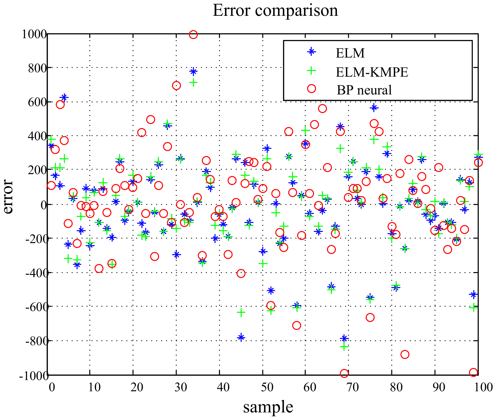
In this subsection, we perform the experiments to verify the prediction performance of the proposed method in comparison to the traditional ELM and BP neural network methods. The ELM wind power prediction results, ELM-KMPE wind power prediction results, and the BP neural network wind power prediction results are shown in Figure 4a,b,c, respectively. Figure 5 shows the error comparison diagram all three algorithms. There are five input variables: wind speed, wind direction, air pressure, temperature, and relative humidity. Five hundred data points are used for model training, and another 100 data points are used for model monitoring and evaluation. It can be seen from the Figure 4 that the predicted value of the selected 100 sample points varies a little from the real value; this is because the results of each operation of the neural network are different, and the average value of 100 training times was adopted.

In this paper, we used the following error criteria: mean absolute error (MAE), mean relative error (MRE), mean square error (MSE), and root mean square error (RMSE).

Table 1. Prediction error between ELM, ELM-KMPE, and BP neural network.

NAME	MAE	MRE	MSE	RMSE
ELM	337.5442	16.6979	245,790.2046	495.7723
ELM-KMPE	255.4860	11.4496	103,612.6563	321.8892
BP neural network	276.2048	15.8444	295,893.7537	543.9612

shows the error comparison of three different prediction methods. It can be seen that the error of ELM-KMPE < BP neural network <ELM. ELM-KMPE is based on the smallest error distribution, because the power distribution of wind power is subject to non-Gaussian distribution, making the smallest possible error and the highest possible precision.

$$MAE=\frac{1}{n}{\displaystyle \sum _{i=1}^n\left|Y_i-{\widehat{Y}}_i\right|}$$

(31)

$$MRE=\frac{1}{n}{\displaystyle \sum _{i=1}^n\left|\frac{Y_i-{\widehat{Y}}_i}{Y_i}\right|}$$

(32)

$$MSE=\frac{1}{n}{\displaystyle \sum _{i=1}^n{\left(Y_i-{\widehat{Y}}_i\right)}^2}$$

(33)

$$RMSE=\sqrt{\frac{1}{n}{{\displaystyle \sum _{i=1}^n\left(Y_i-{\widehat{Y}}_i\right)}}^2}$$

(34)

where $Y_i$ is the ith actual load value, ${\widehat{Y}}_i$ is the ith predicted load value, and n is the total number of predicted points.

4.3.2. Time Complexity Analysis

Time complexity is a key issue for the application of the prediction methods based on neural networks in practice. Therefore, we conducted an experiment to show the time complexity of the proposed method in this subsection.

Table 2. Training time of ELM, ELM-KMPE, and BP neural network.

Name	Training Time(s)
ELM	0.1123
ELM-KMPE	3.6166
BP neural network	2.8017

shows that the training time of the three models is the shortest for ELM, followed by BP neural network, and the training time for ELM-KMPE is the longest. In theory, ELM only needs to take the output weight of the hidden layer, and its input weight and the bias value of the hidden layer are generated randomly. Therefore, there is no need to calculate and the training time is reduced, making it the shortest time. The BP neural network is a neural network based on error feedback. During training, the output error of the upper layer of the neural network should be calculated step by step according to the output error. The ELM-KMPE model requires repeated iterative calculation during training, and it takes the most time to perform 100 iterative operations to ensure the prediction accuracy.

4.3.3. Analysis of the Influence of Hidden Layer Node on the Prediction Results

The number of nodes in the hidden layer of ELM influences the prediction precision of the training model. If there are too many nodes in the hidden layer, this will cause over-learning, poor network adaptability, and a large prediction error. In this paper, after many experiments, the final determination of N is 150 which is most appropriate. As shown in Figure 6 and

Table 3. The MSE results with different number of hidden layer nodes.

N	Error	N	Error	N	Error
10	13832827	110	359306	210	685188
20	5678767	120	384363	220	1095435
30	2762552	130	379956	230	1311510
40	1839047	140	360229	240	1563378
50	1470234	150	343452	250	2430509
60	1036004	160	355909	260	2950694
70	792697	170	373242	270	4621258
80	593769	180	373621	280	8739245
90	438399	190	543456	290	15645062
100	412118	200	632402	300	20876355

, MSE is minimal when the hidden layer node is at 150.

4.3.4. Comparison of Prediction Results after PCA Application

As can be seen from

Table 4. Variance and principal component contribution rate.

Element	Eigenvalue	Variance Contribution Rate/%	Cumulative/%
Wind speed	42.52	42.52	42.52
Wind direction	23.54	23.54	66.06
Temperature	14.55	14.55	80.61
Relative humidity	13.04	13.04	93.65
Air pressure	6.33	6.33	100

, the cumulative contribution rate of variance of the four components of wind speed, wind direction, temperature, and relative humidity is 93.65%, while the contribution rate of variance of air pressure is 6.33%, which accounts for a small proportion. Therefore, wind speed, wind direction, temperature, and relative humidity were selected as the main components.

Figure 7 gives the error diagram before and after principal component extraction. After the principal component extraction, the MSE of the prediction result is 276,003.4592, and the MSE before principal component extraction is 245,790.2046. The difference between the two is small, indicating that the main factors influencing wind power are wind speed, wind direction, temperature, and relative humidity, and that air pressure has little influence on wind power. It can be seen that the PCA algorithm reduces one feature and makes the algorithm simpler and changes little in precision.

4.3.5. The Validation of the Proposed Method via Novel Data Set

To further investigate the performance of the proposed method, a novel data set which was collected from a wind farm in northwest China was used to train the neural network model mentioned above. Solstice was collected every 15 min from 10 October 2016 to 9 April 2018, including the actual power and wind speed data of the wind tower. A total of 52,512 sets of data points was collected. Since there is no other component, the power was predicted only by wind speed. In order to verify the practical significance of the prediction algorithm in this paper, the simulation randomly selected 40,000 data points for training and 10,000 for verification. The error comparison of the three algorithms is shown in

Table 5. Comparison of prediction errors of ELM, ELM- KMPE and BP under new data.

NAME	MAE	MRE	MSE	RMSE
ELM	4.0215	13,320.1620	67.0528	8.1886
ELM-KMPE	3.8211	13,276.7444	67.0085	8.1859
BP neural network	4.0305	13,349.4341	71.2589	8.4415

below. It can be seen that that error of the three algorithm is the best result of ELM-KMPE in case of numerous data, and the other two algorithm errors are in close proximity.

5. Conclusions

Considering the non-linear and non-Gaussian features of wind power, a novel wind power prediction scheme based on ELM with KMPE was proposed in this work. The KMPE is a robust loss function designed by MPE in kernel space, and it is introduced into ELM to replace the MSE loss in the original form of ELM, which can improve the performance of the ELM when the data are non-linear and non-Gaussian. Therefore, by using the ELM with KMPE, we could achieve a higher prediction accuracy. In addition, taking into account many influencing factors for wind power prediction, we used PCA analysis only to select main factors—wind speed, wind direction, relative humidity, and air pressure—to predict the wind power, so as to reduce the computational complexity of the proposed approach. The experiment includes error analysis with different error criteria, time complexity of the three algorithms, a selection of the optimal number of hidden nodes, an elimination of redundant elements in the data, and an expansion of five major parts of the data. The first part compared and evaluated the effectiveness of wind power prediction methods under different conditions, using traditional ELM and BP neural network methods. The experimental results show that the proposed ELM-KMPE method is superior to other methods. In the second part, it could be seen that ELM-KMPE also has its disadvantages, that is, the calculation speed is the slowest because of the fixed point iteration. In the third part, the influence of the number of hidden neurons on the prediction accuracy was investigated and the optimal number is 150. In the fourth part, the PCA algorithm was adopted to eliminate redundant factors (air pressure) and simplify the complexity of the algorithm. The fifth part verified the algorithm with another set of experimental data to prove its effectiveness.

Although the proposed method can achieve ideal predictive performance, there is still much work to be done in this research direction: (1), different optimization algorithms (such as particle swarm optimization, genetic algorithm, simulated annealing algorithm, etc.) can be adopted for the weight matrix or vector in the neural network; (2) the calculation complexity of the proposed method should be improved; (3) with better future computer hardware, deep learning, cyclic neural networks, and convolutional neural networks can be used to predict wind power and investigate its prediction performance.

References

- Kusiak, A.; Zheng, H.; Zhe, S. Short-Term Prediction of Wind Farm Power: A Data Mining Approach. IEEE Trans. Power Appar. Syst. 2009, 24, 125–136. [Google Scholar] [CrossRef] [Green Version]
- Ding, Y.Y.; Zhou, H.; Tan, Z.; Chen, Y.; Ding, J. The influence of wind direction on short-term wind power prediction: A case study in north China. In Proceedings of the IEEE PES Innovative Smart Grid Technologies, Tianjin, China, 21–24 May 2012; pp. 1–5. [Google Scholar]
- Huo, Y.; Jiang, P.; Zhu, Y.; Feng, S.; Wu, X. Optimal Real-Time Scheduling of Wind Integrated Power System Presented with Storage and Wind Forecast Uncertainties. Energies 2015, 8, 1080–1100. [Google Scholar] [CrossRef] [Green Version]
- Cruz, M.; Fitiwi, D.; Santos, S.; Mariano, S.; Catalão, J. Prospects of a Meshed Electrical Distribution System Featuring Large-Scale Variable Renewable Power. Energies 2018, 11, 3399. [Google Scholar] [CrossRef]
- Li, C.P.; Zhang, S.N.; Zhang, J.X.; Qi, J.; Li, J.; Guo, Q.; You, H. Method for the Energy Storage Configuration of Wind Power Plants with Energy Storage Systems used for Black-Start. Energies 2018, 11, 3394. [Google Scholar] [CrossRef]
- Yun, P.P.; Ren, Y.F.; Xue, Y. Energy-Storage Optimization Strategy for Reducing Wind Power Fluctuation via Markov Prediction and PSO Method. Energies 2018, 11, 3393. [Google Scholar] [CrossRef]
- Tascikaraoglu, A.; Uzunoglu, M. A review of combined approaches for prediction of short-term wind speed and power. Renew. Sustain. Energy Rev. 2014, 34, 243–254. [Google Scholar] [CrossRef]
- Khalid, M.; Savkin, A.V. A Method for Short-Term Wind Power Prediction with Multiple Observation Points. IEEE Trans. Power Syst. 2012, 27, 579–586. [Google Scholar] [CrossRef]
- Gugliani, G.K.; Sarkar, A.; Ley, C.; Mandal, S. New Methods to Assess Wind Resources in Terms of Wind Speed, Load. Power and Direction. Renew. Energy 2018, 129A, 168–182. [Google Scholar] [CrossRef]
- Bai, G.X.; Ding, Y.W.; Yildirim, M.B.; Ding, Y.H. Short-term prediction models for wind speed and wind power. In Proceedings of the 2014 2nd International Conference on Systems and Informatics (ICSAI 2014), Shanghai, China, 15–17 November 2014; pp. 180–185. [Google Scholar]
- Yao, Q.; Liu, Y.; Zhang, W.; Hu, Y. Study on the comprehensive evaluation method of regional wind power prediction. In Proceedings of the 2017 36th Chinese Control Conference (CCC), Dalian, China, 26–28 July 2017; pp. 10259–10264. [Google Scholar]
- Chen, K.; Yu, J. Short-term wind speed prediction using an unscented Kalman filter based state-space support vector regression approach. Appl. Energy 2014, 113, 690–705. [Google Scholar] [CrossRef]
- Zuluaga, C.D.; Álvarez, M.A.; Giraldo, E. Short-term wind speed prediction based on robust Kalman filtering: An experimental comparison. Appl. Energy 2015, 156, 321–330. [Google Scholar] [CrossRef]
- Cao, Y.L.; Liu, Y.H.; Zhang, D.Y.; Wang, W.; Chen, Z. Wind power ultra-short-term forecasting method combined with pattern-matching and ARMA-model. In Proceedings of the Powertech IEEE 2013, Grenoble, France, 16–20 June 2013; pp. 1–4. [Google Scholar]
- Zhang, J.Y.; Wang, C. Application of ARMA Model in Ultra-short Term Prediction of Wind Power. In Proceedings of the 2013 International Conference on Computer Sciences and Applications, Wuhan, China, 14–15 December 2013; pp. 361–364. [Google Scholar]
- Li, J.X.; Mao, J.D. Ultra-short-term wind power prediction using BP neural network. In Proceedings of the Industrial. 2014 9th IEEE Conference on Industrial Electronics and Applications, Hangzhou, China, 9–11 June 2014; pp. 2001–2006. [Google Scholar]
- Zhu, L.; Shi, H.T.; Ding, M.S. A Chaotic BP Neural Network Used to Wind Power Prediction. In Proceedings of the 2018 2nd IEEE Advanced Information Management, Communicates, Electronic and Automation Control Conference (IMCEC), Xi’an, China, 25–27 May 2018; pp. 1169–1172. [Google Scholar]
- Zhang, G.; Zhang, L.; Xie, T. Prediction of short-term wind power in wind power plant based on BP-ANN. In Proceedings of the 2016 IEEE Advanced Information Management, Communicates, Electronic and Automation Control Conference (IMCEC), Xi’an, China, 3–5 October 2016; pp. 75–79. [Google Scholar]
- Bessa, R.J.; Miranda, V.; Gama, J. Entropy and Correntropy against Minimum Square Error in Offline and Online Three-Day Ahead Wind Power Forecasting. IEEE Trans. Power Syst. 2009, 24, 1657–1666. [Google Scholar] [CrossRef]
- Damousis, I.G.; Dokopoulos, P. A fuzzy expert system for the forecasting of wind speed and power generation in wind farms. In Proceedings of the PICA 2001. Innovative Computing for Power—Electric Energy Meets the Market. 22nd IEEE Power Engineering Society. International Conference on Power Industry Computer Applications (Cat. No.01CH37195), Sydney, NSW, Australia, 20–24 May 2001; pp. 63–69. [Google Scholar]
- Damousis, I.G.; Alexiadis, M.C.; Theocharis, J.B.; Dokopoulos, P.S. A fuzzy model for wind speed prediction and power generation in wind parks using spatial correlation. IEEE Trans. Energy Convers. 2004, 19, 352–361. [Google Scholar] [CrossRef]
- Dong, W.; Yang, Q.; Fang, X.L. Multi-Step Ahead Wind Power Generation Prediction Based on Hybrid Machine Learning Techniques. Energies 2018, 11, 1975. [Google Scholar] [CrossRef]
- Neeraj, B.; Andrés, F.; Daniel, V.; Kulat, K. A Novel and Alternative Approach for Direct and Indirect Wind-Power Prediction Methods. Energies 2018, 11, 2923. [Google Scholar] [CrossRef]
- Shi, X.Y.; Lei, X.W.; Huang, Q.; Huang, S.; Ren, K.; Hu, Y. Hourly Day-Ahead Wind Power Prediction Using the Hybrid Model of Variational Model Decomposition and Long Short-Term Memory. Energies 2018, 11, 3227. [Google Scholar] [CrossRef]
- Quan, H.; Srinivasan, D.; Khosravi, A. Short-term load and wind power forecasting using neural network-based prediction intervals. IEEE Trans. Neural Netw. Learn. Syst. 2017, 25, 303–315. [Google Scholar] [CrossRef]
- Huang, G.B.; Zhu, Q.Y.; Siew, C.K. Extreme learning machine: Theory and applications. Neurocomputing 2006, 70, 489–501. [Google Scholar] [CrossRef] [Green Version]
- Huang, G.; Huang, G.B.; Song, S.; You, K. Trends in extreme learning machines: A review. Neural Netw. 2015, 61, 32–48. [Google Scholar] [CrossRef]
- Wang, X.Y.; Han, M. Online sequential extreme learning machine with kernels for nonstationary time series prediction. Neurocomputing 2014, 145, 90–97. [Google Scholar] [CrossRef]
- Sun, W.; Zhang, C.C. A Hybrid BA-ELM Model Based on Factor Analysis and Similar-Day Approach for Short-Term Load Forecasting. Energies 2018, 11, 1282. [Google Scholar] [CrossRef]
- Cornejo-Bueno, L.; Cuadra, L.; Jiménez-Fernández, S.; Acevedo-Rodríguez, J.; Prieto, L.; Salcedo-Sanz, S. Wind Power Ramp Events Prediction with Hybrid Machine Learning Regression Techniques and Reanalysis Data. Energies 2017, 10, 1784. [Google Scholar] [CrossRef]
- Alexandre, E.; Cuadra, L.; Nieto-Borge, J.C.; Candil-Garcia, G.; Del Pino, M.; Salcedo-Sanz, S. A hybrid genetic algorithm-extreme learning machine approach for accurate significant wave height reconstruction. Ocean Model. 2015, 92, 115–123. [Google Scholar] [CrossRef]
- Mohammadi, K.; Shamshirband, S.; Yee, P.L.; Petković, D.; Zamani, M.; Ch, S. Predicting the wind power density based upon extreme learning machine. Energy 2015, 86, 232–239. [Google Scholar] [CrossRef]
- Wan, C.; Xu, Z.; Pinson, P.; Dong, Z.Y.; Wong, K.P. Probabilistic Forecasting of Wind Power Generation Using Extreme Learning Machine. IEEE Trans. Power Syst. 2014, 29, 1033–1044. [Google Scholar] [CrossRef] [Green Version]
- Mishra, S.P.; Dash, P.K. Short term wind power forecasting using Chebyshev polynomial trained by ridge extreme learning machine. In Proceedings of the 2015 IEEE Power, Communication and Information Technology Conference (PCITC), Bhubaneswar, India, 15–17 October 2015; pp. 173–177. [Google Scholar]
- Ahlstrom, M.L.; Zavadil, R.M. The Role of Wind Forecasting in Grid Operations & Reliability. In Proceedings of the 2005 IEEE/PES Transmission & Distribution Conference & Exposition: Asia and Pacific, Dalian, China, 18 August 2005; 2005; pp. 1–5. [Google Scholar]
- Costa, A.; Crespo, A.; Navarro, J.; Lizcano, G.; Madsen, H.; Feitosa, E. A review on the young history of the wind power short-term prediction. Renew. Sustain. Energy Rev. 2008, 12, 1725–1744. [Google Scholar] [CrossRef] [Green Version]
- Chen, B.D.; Xing, L.; Xu, B.; Zhao, H.; Zheng, N.; Principe, J.C. Kernel Risk-Sensitive Loss: Definition. Properties and Application to Robust Adaptive Filtering. IEEE Trans. Signal Process. 2017, 65, 2888–2901. [Google Scholar] [CrossRef]
- Liu, W.F.; Pokharel, P.P.; Principe, J.C. Correntropy: Properties and Applications in Non-Gaussian Signal Processing. IEEE Trans. Signal Process. 2007, 55, 5286–5298. [Google Scholar] [CrossRef]
- Chen, B.D.; José, C. Maximum Correntropy Estimation Is a Smoothed MAP Estimation. IEEE Signal Process. Lett. 2012, 19, 491–494. [Google Scholar] [CrossRef]
- Chen, B.D.; Xing, L.; Liang, J.L.; Zheng, N.; Principe, J.C. Steady-State Mean-Square Error Analysis for Adaptive Filtering under the Maximum Correntropy Criterion. IEEE Signal Process. Lett. 2014, 21, 880–884. [Google Scholar] [CrossRef]
- Sideratos, G.; Hatziargyriou, N.D. An Advanced Statistical Method for Wind Power Forecasting. IEEE Trans. Power Syst. 2007, 22, 258–265. [Google Scholar] [CrossRef]
- Chen, B.D.; Xing, L.; Wang, X.; Qin, J.; Zheng, N. Robust Learning With Kernel Mean p-Power Error Loss. Energy Conv. Manag. 2018, 48, 2101–2113. [Google Scholar] [CrossRef]
- Tang, P.; Chen, D.; Hou, Y. Entropy method combined with extreme learning machine method for the short-term photovoltaic power generation forecasting. Chaos Solitons Fractals 2016, 89, 243–248. [Google Scholar] [CrossRef]
- Baldi, P.; Hornik, K. Neural networks and principal component analysis: Learning from examples without local minima. Neural Netw. 1989, 2, 53–58. [Google Scholar] [CrossRef]
- Eastment, H.T.; Krzanowski, W.J. Cross-Validatory Choice of the Number of Components from a Principal Component Analysis. Technometrics 1982, 24, 73–77. [Google Scholar] [CrossRef]
- Wang, Y.N.; Xie, D.; Wang, X.T.; Zhang, Y. Prediction of Wind Turbine-Grid Interaction Based on a Principal Component Analysis-Long Short Term Memory Model. Energies 2018, 11, 3221. [Google Scholar] [CrossRef]
- Akdağ, S.A.; Bagiorgas, H.S.; Mihalakakou, G. Use of two-component Weibull mixtures in the analysis of wind speed in the Eastern Mediterranean. Appl. Energy 2010, 87, 2566–2573. [Google Scholar] [CrossRef]
- Mohammadi, K.; Alavi, O.; Mostafaeipour, A.; Goudarzi, N.; Jalilvand, M. Assessing different parameters estimation methods of Weibull distribution to compute wind power density. Energy Convers. Manag. 2016, 108, 322–335. [Google Scholar] [CrossRef]
- Yeh, T.H.; Wang, L. A Study on Generator Capacity for Wind Turbines Under Various Tower Heights and Rated Wind Speeds Using Weibull Distribution. IEEE Trans. Energy Convers. 2008, 23, 592–602. [Google Scholar] [CrossRef]
- Alexiadis, M.C.; Dokopoulos, P.S.; Sahsamanoglou, H.S. Wind speed and power forecasting based on spatial correlation models. IEEE Trans. Energy Convers. 1999, 14, 836–842. [Google Scholar] [CrossRef]
Figure 1.
ELM structure diagram.
Figure 2.
ELM-KMPE structure diagram.
Figure 3.
A schematic representation of the research workflow.
Figure 4.
The real value of wind power is compared with the predicted value. (a) ELM (b) ELM-KMPE (c) BP neural network.
Figure 5.
Comparison diagram of three algorithm errors.
Figure 6.
The MSE results with different number of hidden layer nodes.
Figure 7.
The error of the ELM-KMPE method before and after principal component extraction.