On the Variation of Turbulence in a High-Velocity Tidal Channel

Abstract

This study presents the variation in turbulence parameters derived from site measurements at a tidal energy test site. Measurements were made towards the southern end of the European Marine Energy Centre’s tidal energy test site at the Fall of Warness (Orkney, Scotland). Four bottom mounted divergent-beam Acoustic Doppler Current Profilers (ADCPs) were deployed at three locations over an area of 2 km by 1.4 km to assess the spatial and temporal variation in turbulence in the southern entrance to the channel. During the measurement campaign, average flood velocities of 2 ms⁻¹ were recorded with maximum flow speeds of 3 ms⁻¹ in the absence of significant wave activity. The velocity fluctuations and turbulence parameters show the presence of large turbulent structures at each location. The easternmost profiler located in the wake of a nearby headland during ebb tide, recorded flow shielding effects that reduced velocities to almost zero and produced large turbulence intensities. The depth-dependent analysis of turbulence parameters reveals large velocity variations with complex profiles that do not follow the standard smooth shear profile. Furthermore, turbulence parameters based on data collected from ADCPs deployed in a multi-carrier frame at the same location and time period, show significant differences. This shows a large sensitivity to the make and model of ADCPs with regards to turbulence. Turbulence integral length scales were calculated, and show eddies exceeding 30 m in size. Direct comparison of the length scales derived from the streamwise velocity component and along-beam velocities show very similar magnitudes and distributions with tidal phase.

1. Introduction

As tides pass through narrow channels and around headlands, high-velocity flows are produced. Depending on site-specific characteristics, the turbulence of these flows varies in time and space. When these turbulent flows encounter a tidal stream turbine (TST), the severity of turbulence affects the turbine energy extraction capability by altering blade performance. This results in reduced rotor thrust and torque [1], which causes a detriment in turbine performance of over 10%. Prolonged exposure to high turbulent flows increases fatigue load cycles and blade bending [2], thereby reducing the expected lifespan of a turbine. Mitigation techniques can be applied to keep design tolerances high to account for turbulence related stresses, but this also increases manufacturing costs. The quantification of turbulence remains an important factor in the optimization of energy extraction and turbine durability and thus successful tidal stream developments.

The measurement of turbulence in a fluid, at scales relevant to rotating hydrofoils, by its nature requires high-resolution measurements (>1 Hz). Originally, sensors were developed to determine atmospheric turbulence; these were designed to be unobtrusive, where the measurements do not cause disruption to the flow of the fluid. To achieve this, the principle of Doppler shift was applied. This transmits high-frequency bursts (pings) from three or more transceivers. As the sound is scattered off by suspended moving particles in the fluid, a frequency shift is observed. This shift in frequency uses the Doppler effect formula, where the particle velocity, and therefore fluid velocity, can be calculated. The combination of multiple beams on different axes allows for the velocity calculation in the x, y and z vectors and therefore speed and direction. This was originally done for converging beam sensors [3]. This technology was later applied to the ocean environment [4], where an adapted method for calculating seabed friction velocity was presented for low flow speeds in the presence of waves. Acoustic Doppler Velocimeters (ADVs) offer high-resolution sample rates in the order of 10 Hz assuming a small volume flow homogeneity (5–50 mm) [5]. However, due to the focusing of the beams, a small area can only be observed, and this limits these sensors to small profiles or single point measurements. When the beam angle configuration changes from convergent to divergent, the beams cover a much larger area. If a similar homogenous flow approximation is applied, but now over an area of 1–50 m, then the component flow directions can be calculated for a depth profile. The application of this method has been used for many years in divergent beam ADCPs. Originally operating via “Narrow-Band” acoustic pulses, instantaneous velocity measurements experienced high noise levels, limiting these datasets to time averaged results not suitable for turbulence assessment. The development of “Broadband” acoustic processing has allowed more accurate instantaneous velocity measurements for diverging beam sensors [6,7]. This continues to allow velocity measurements to be made throughout the water column, but with much higher sample rates, without the need for temporal averaging. For some sensors, this means sample rates as high as 10 Hz or above can be used while maintaining low data noise levels.

The number of transceivers on a sensor has increased over the years. While it is possible to get velocity measurements from a single beam, the velocity component is only in the beam direction, providing heavy application restrictions. Three transducers were common for a number of years and this allowed the calculation of directional velocity components. When combined with a pressure sensor, surface waves could also be measured. This used the pressure, u and v velocity (PUV) method to measure the surface elevation using the pressure sensor and the wave directional orbital velocity (u and v) to establish wave direction [8]. The introduction of four beam sensors with opposing angled beams on two perpendicularly aligned axis increased the accuracy of flow measurements. This allowed two measurements to be used to calculate the velocity in each horizontal vector. More recently, five beam sensors have become the new standard. These use the same beam orientation as the four beam sensors; where the introduction of a fifth vertical beam allows a direct measurement of the vertical velocity and surface elevation. While the implementation of a fifth beam and acoustic surface tracking isn’t new, it is now more commonplace and integrated as default in a wide range of standard ADCPs.

The calculation of turbulence parameters from beam velocities of a 4-beam ADCP in relatively slow velocities (<1 ms⁻¹) was demonstrated in [8]. This identified the effects of Doppler noise and its implications on turbulence parameters. The Doppler noise is created as a byproduct of the velocity calculation, where a phase difference for the Doppler shift occurs for multiple returns within a spatially determined cell [9]. More recent studies quantifying turbulence in tidal channels compared the velocities between a bed-mounted ADCP and an ADV [10,11]. These studies presented a standardised metric, adopted from the wind energy industry, to quantify tidal turbulence; this is known as the turbulence intensity. The turbulence intensity can be calculated using the velocity fluctuation minus the Doppler noise. If the noise is not accounted for, the instantaneous measurements from ADCPs can overestimate the value of the standard deviation calculated from velocity. This produces higher turbulence values for the same corresponding location. The noise can be described as white noise, where it is distributed evenly across all frequencies. The effects of this noise can be mitigated by averaging; this can either be done in time, where instantaneous velocity fluctuations are averaged over a number of minutes, or in space, where velocity fluctuations can be averaged across the vertical profile. This, however, is not a viable solution when considering turbulence measurements. The quantification of the Doppler noise was improved in [12]; this applied a polynomial least square regression method to extend the inertial range to the high-frequency end of the velocity spectrum, lowering the noise floor. Additional methods for correcting instrument noise were presented in [13]. These use either a Noise Auto-Correlation (NAC) or Proper Orthogonal Decomposition (POD) approach to determine and remove noise. In the case of the NAC method, the noise level is calculated based on the velocity spectrum, restricting the noise reduction to the frequency domain. However, the POD method is capable of reducing noise over the spectrum and within the time domain, providing a more flexible output. In addition, these methods may be more suitable for reducing noise in the presence of waves.

The number of published studies quantifying turbulence levels using in-situ field measurements at tidal energy test sites has increased in recent years [14,15,16,17,18,19,20]. Similar studies have been conducted in rivers [21,22,23], however, due to differences on the onset flow conditions, topography and sedimentation, the results of these studies is of limited relevance. Both the tidal and river studies use divergent beam ADCPs to record the velocity fluctuations. Alternatively, single-beam Doppler profilers, horizontally mounted and aligned with the in-stream velocity direction, have been used for turbulence assessment [18,24]. This configuration provides streamwise velocity fluctuations with no assumption of flow homogeneity, resulting in a more accurate measurement of ambient flow speeds at mid-water depth and turbine hub height. However, additional single beam profilers are required (as installed in [18]) to provide flow information in the transverse and vertical directions. The previous studies provide a basic resource assessment, where flow velocities and directions are first quantified in time and often depth. Then a range of turbulence parameters are presented including the standard deviation of the velocity fluctuations, turbulence intensity, Reynolds stresses, Turbulence Kinetic Energy and velocity spectra. Previous studies also provide benchmarks to other locations that allow the Fall of Warness to be contextualized in terms of other potential tidal test sites.

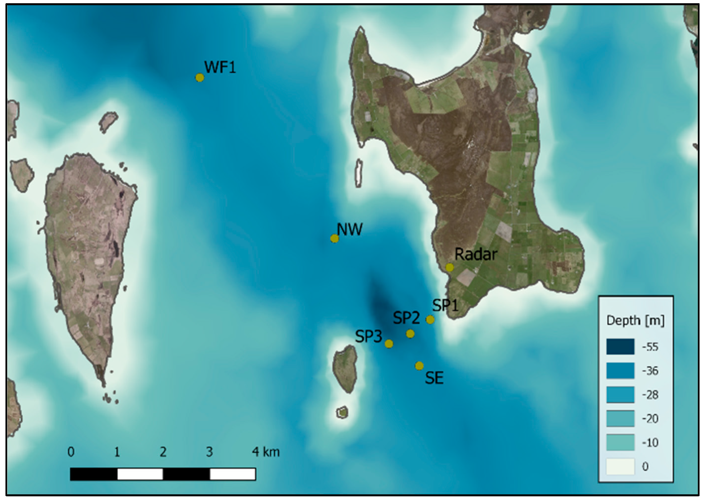
In this study, data are presented from a sensor network at the southern end of the Fall of Warness, with the locations specified in Figure 1. The diverging acoustic Doppler profilers (D-ADP) were deployed simultaneously to measure wave and currents over a 4 day period. The general resource and turbulence characteristics are calculated and compared for each sensor with depth and time. Specific emphasis is placed on the peak velocities of the flood and ebb tides and the average conditions, where turbulence interactions are likely to be higher. The turbulence intensity, turbulence spectrum, Reynolds stresses and integral time and length scales are presented. A direct comparison between the homogenous approximated length scale and the raw beam length scales are presented for two sensors. The data analysis indicates that along with spatial and temporal variations, sensor make and model specific features also cause variation in observed turbulence parameters. These differences are highlighted and discussed throughout this paper. The presentation of turbulence intensity and length scale provide important boundary conditions required for the simulation of tidal turbines [25]. This is crucial for the long term performance analysis of a single or array of devices.

2. Data Collection and Methodology

2.1. Sensor Deployment

A measurement campaign was devised to simultaneously operate multiple coastal sensors at six locations between the dates of the 13th and 18th of June 2016. To enable the measurement of turbulence parameters, at scales relevant to tidal stream turbines, a continuous time series recording at a sample rate of 0.5 Hz or higher is required. Only four of these sensors were suitable for turbulence analysis and these are discussed in this paper. Work was carried out as part of the Response of Tidal Energy Converters to Combined Tidal Flow, Waves, and Turbulence (FloWTurb) project (EPSRC EP/N021487/1). All sensor locations are shown in Figure 1 and discussed in this paper are SP1, SP3 and SE, where the SE location features multiple sensors deployed in a single frame. Names, depths and sampling information of the relevant sensors are shown in

Table 1. Sensor specifications.

Sensors	Location	Beams	Transmitting Frequency	Beam Angle	Sample Frequency	Vertical Cell Size	Depth
Signature 500	SE	5	500 kHz	25°	4 Hz	0.5 m	37 m
Signature 1000	SP1	5	1000 kHz	25°	4 Hz	0.5 m	37 m
RDI Sentinel 600	SE	4	600 kHz	20°	2 Hz	0.75 m	37 m
RDI Sentinel 600	SP3	4	600 kHz	20°	0.5 Hz	1 m	44 m

.

The sensors were located at the southern end of the channel within an area of approximately 2 km (along the channel length) by 1.4 km (perpendicular to the channel length). The bathymetry data used in Figure 1 is taken from the UK Hydrographic Office [26]. Each deployment location uses a bottom mounted ADCP housed in a stainless steel frame. A dual-axis gimbal was used to mount each sensor within the frame. The total dry mass of each frame is around 400 kg. In addition, a land-based X-band radar system was used for remote measurement of wave and surface current conditions; further details on the measurement of the flow characteristics using the radar can be found in [27]. The sensors used were the Signature 500 and Signature 1000 manufactured by Nortek (Rud, Norway), and two Workhorse Sentinel 600 ADCPs manufactured by Teledyne RDI (Poway, CA, USA).

The sensor specifications and setup are shown in Table 1. The SP2 sensor was lost on retrieval and therefore no data exists. An additional Waverider DWR-G4 wave buoy (Datawell, Heerhugowaard, The Netherlands) was attached to the SE sensor frame. This provided surface wave information during slack water periods as the ADCP’s fifth vertical beam was not enabled. This reduced internal processing time and power consumption for the ADCPs. In order to minimize interference between the four co-located SE sensors (1 MHz Nortek AWAC, 400 kHz Nortek Aquadopp, RDI Sentinel 600 and Nortek Signature 500, the latter two of which are suitable for turbulence characterisation) i.e., sensor crosstalk, each sensor suitable for turbulence characterisation recorded data in a staggered formation, permitting only one sensor operated at any one time. This allowed each sensor to record for 20 min of data, then remain inactive for 40 min while each sensor in turn sampled the water column. When all the data is stitched together from each sensor a continuous measurement of the flow is obtained. The deployment period was scheduled between a neap and a spring tide, where the current velocities were increasing.

2.2. Basic Data Processing

Due to the simultaneous deployment of these sensors, it was not possible to standardise either the sensor type or sampling regime for all the deployment locations. This prevented the use of standard sensor specific processing tools, as the subtle differences in the manufacturer’s post-processing procedures may impede the direct comparison of data. To account for this, new software was developed in MATLAB (version R2018a) to read and process raw data from both Teledyne or Nortek sensors. All sensors have a minimum of four diverging beams with beam angles as shown in Table 1. Sensors with an additional fifth beam are capable of surface measurements using acoustic surface tracking. However, the focus of these deployments was on the current data collection, so no vertical beam data were recorded. In order to measure current velocities, the Doppler effect is used based on the frequency shift between emitted and received pulses along each divergent beam. While many previous studies use beam velocities to calculate horizontal velocities and turbulence metrics, the orientation of the beam to the flow is vital, as a misrepresentative value will be recorded and a large difference from the opposing beam will be seen if the beam is not directly in line with the flow direction. This study applies an approach where the velocities from four beams are used to calculate the flow vector in a number of coordinate systems [28,29]. These coordinate systems are shown in Figure 2.

The three coordinate systems used for the calculation of flow and turbulence parameters are xyz relative to beam 1, enu (East, North and Up) relative to magnetic north, and streamwise relative to the mean flow direction (uvw). For this study, a short-term 600 s average was used to calculate mean flow direction. Equation (1) shows the method of calculating the relative directional flow using the sensor orientation (xyz) depending on the beam angle $\left(\theta \right)$:

$$\left[\begin{array}{c}x\\ y\\ z\end{array}\right]=\left[\begin{array}{c}\left(b1-b3\right)/(2\sin \left(\theta )\right)\\ \left(b2-b4\right)/(-2\sin \left(\theta )\right)\\ \left(b1+b2+b3+b4\right)/(4\cos \left(\theta )\right)\end{array}\right]$$

(1)

In Equation (1) b1–b4 are the beam velocities from each transducer in a clockwise rotation. This is consistent with Nortek’s beam numbering convention, and results from the Teledyne sensors were rearranged to fit this convention. To correct for sensor misalignment on installation and sensor motion during deployment, a coordinate transform was applied to each sampled measurement, utilizing the instrument’s onboard tilt sensors and magnetic compass, where the velocities are multiplied by a tilt matrix (R) based on three degrees of freedom, heading (hh), pitch (pp) and roll (rr). This is shown in Equation (2) and the transformation to Earth coordinates is shown in Equation (3):

$$R=\left[\begin{array}{ccc}\cos \left(hh\right)& \sin \left(hh\right)& 0\\ -\sin \left(hh\right)& \cos \left(hh\right)& 0\\ 0& 0& 1\end{array} \right]\left[\begin{array}{ccc}\cos \left(pp\right)& -\sin \left(pp\right)\sin \left(rr\right)& -\cos \left(rr\right)\sin \left(pp\right)\\ 0& \cos \left(rr\right)& -\sin \left(rr\right)\\ \sin \left(pp\right)& \sin \left(rr\right)\cos \left(pp\right)& \cos \left(pp\right)\cos \left(rr\right)\end{array}\right]$$

(2)

$$enu=R\times xyz$$

(3)

This orientates the velocity vectors to Earth coordinates. The uvw velocities are calculated based on the same 600 s window, where the average flow direction is subtracted from the enu flow directions. This provides a speed and direction relative to the streamwise velocity. The vectors are then calculated using the speed multiplied by the cosine of the new streamwise and transverse directions. For the analysis of flow around a tidal stream turbine, the uvw coordinate system is deemed the most relevant, as velocity fluctuations are in line with the turbine hub and perpendicular to the rotor disk. The calculation of the velocity components uses multiple diverging directional beams, this produces a cone-shaped sample area that is narrower at the seabed near the sensor head and expands towards the sea surface based on the transceiver beam angle. In order to calculate the velocity components, it must be assumed that the current flow is homogeneous across the plane of all beams, which is a clear weakness in the use of coordinate transforms for turbulence assessment. The size of this plane increases with distance away from the sensor, which in turn increases the size of the area of the homogeneous approximation. This subsequently increases the size of the minimum resolvable flow structure. While this is a considerable limitation when measuring turbulence, it allows for a simple deployment process where the sensor can be placed on uneven ground without fine positioning to align beam 1 with north. Continuous monitoring of sensor pitch, roll and yaw also allows for compensation of any unexpected frame movements, which are not uncommon in higher velocity environments.

3. Data Analysis and Results

3.1. Flow Characteristics

The average flow characteristics from the high-resolution sensors deployed in the Fall of Warness are shown in Figure 3. The uvw velocity vectors are plotted based on a 600 s average, from a start date of 11:00:00 13/07/2017 and are based on data collected over the following four days. The streamwise velocity vector for all sensors shows a periodic fluctuation as a result of the flood and ebb tide, where one complete tidal cycle is composed of two neighbouring peaks in the streamwise velocity. This is indicative of a semidiurnal tidal cycle. The initial peak in the SE—Signature 500 and SP3 Sentinel 600 velocities, depicts the first flood tide, after which the lower magnitude ebb tide follows. This pattern is not the case for the SP1 sensor, where the peaks are shown to occur in the initial part of the flood tides and no obvious peak in the ebb tide is observed. The positive transverse velocity indicates the deviation from the streamwise flow in a clockwise direction and a negative value equates to an anticlockwise deviation. As expected, the u velocity far exceeds the v velocity for all sensors. The flow directions, relative to magnetic north, and speed at 10 m above the seabed are plotted on the right side of Figure 3. The results indicate similar tidal ellipses for the SE and SP3 sensors. The tidal ellipse shape for these sensors is particularly compressed, indicating an almost bidirectional flow pattern, where the flood tide experiences higher velocities towards a south-south-easterly direction (150°). The tidal ellipse for the SP1 sensor shows much larger directional variation, with a small broad peak for the flood tide and no peak velocity for the ebb tide. This is caused by the close proximity of the sensor to the southern headland of the isle of Eday and related generation of large eddies during ebb tide at the sensor location.

3.2. Depth Profiles

The velocity distribution with depth is presented in Figure 4. This shows the peak flood and ebb tides, based on the maximum velocities over the 600 s windows, for the first 3 respective tidal phases for each sensor. This is conducted for combined speed (uvw), streamwise (u), transverse (v) and vertical (w) velocity components, where the average speed profile indicates the net combined velocity at each depth interval. To visually separate each tidal phase, the flood tide has been plotted as positive (blue) and the ebb tide is shown as negative (red). Distance above the seabed (z) is used to describe the vertical cell position, where the first bin height was set at approximately 2 m for all sensors. In addition to a directional dependence of the velocity magnitudes as shown in Figure 3, the velocity shear profiles in Figure 4 also show reductions in flow speeds toward the sea bed in various degrees of magnitude. The variation in profile is caused as a result of spatial and tidal phase differences, but for the co-located sensor, different flow profiles are seen at the same location between the different sensor types. The SE—Signature 500 sensor shows a typical shear profile from the seabed to 19 m upward, where the current velocity consistently increases. From 19 m to 26 m a considerable reduction in flow speed occurs, and this was also confirmed by looking at the individual beam-by-beam velocities. The co-located SE-RDI Sentinel sensor does not replicate this flow feature and shows a smooth gradually increasing velocity shear profile. Further observational differences identify a substantial variation in the proportion of velocity components, u and v for the SE sensors. This shows the Signature sensor recording a much greater transverse velocity. Both sensor manufacturers have been contacted with regards to the quality of the data sets, the outcome of this suggested that no errors were contained within either data set. Both manufactures were fully satisfied with the quality of their sensor specific data sets. The SP1 sensor shows very different profiles for flood and ebb, where the flood shows a rapid change in the velocity gradient near the seabed and a uniform flow speed of 1.3 ms⁻¹ with only a small increase towards the surface. The ebb tide shows very small velocities for the lower part of the water column, and this changes after 13 m upwards, where the velocity increases gradually towards the surface. The SP3 sensor shows a much more conventional shear profile, which experiences a smooth curve from the seabed to the surface, where flow speeds continually increase. The velocity profiles presented provide further details of the flow characteristics around the Fall of Warness. These measurements are key to fully understanding the following analysis of turbulence parameters.

3.3. Turbulence Intensity

To quantify the turbulence levels, the commonly used turbulence intensity ($I_u$) is calculated. The method used in this paper uses Equation (4) as presented in [11]:

$$I_u=\frac{\sqrt{\langle u^{\prime 2}\rangle -{\sigma }_{noise}^2}}{\overline{u}}$$

(4)

where $u$ is the streamwise velocity component and $\overline{\mathrm{u}}$ is the mean streamwise velocity. $\langle u^{\prime 2}\rangle$ is the velocity variance, and ${\sigma }_{noise}^2$ is the Doppler noise from the sensor. The distribution of the Doppler noise is spread evenly across all frequencies. As the high frequency regions of the spectrum have comparably less energy than the lower frequencies, this results in a larger relative noise level for the high frequency turbulence measurements. To account for this increased instrument noise the method described in [12] was applied to quantify the noise variation. This calculates a ${\sigma }_{noise}^2$ based on an extended fit of the turbulence spectrum. This is only possible by applying Kolmogorov’s theory of the inertial range; this states that inertial effects are much greater than any viscous effects and suggests a rate of turbulence energy decay of −5/3 [30]. This only remains valid in the absence of waves. A Welch’s Fast Fourier Transformation (FFT) was applied to quantify the power spectral density of the turbulence time series in the frequency domain. Each continual time series, or ensemble, was separated into window lengths of 200 s, and a Hanning filter was applied to each window. Zero padding was added to increase the number of samples to equal the next power of the total number of samples. If the ${\sigma }_{noise}^2$ value is set to 0, no noise reduction is applied for the turbulence intensity and the calculation becomes the same as the standard calculation [31]. The definition of $\overline{u}$ is sometimes described as the mean flow velocity at the turbine hub height. As this study is not turbine device specific the more flexible definition is applied, this specifies $\overline{u}$ as average streamwise velocity for each depth interval. The calculated turbulence intensity data from the sensor campaign is presented in Figure 5.

When the results are reviewed in combination with the velocity time series (Figure 3), the higher turbulence intensities are associated with the slower velocities (near slack water) and the lower turbulence intensities with the flood and ebb phases. This is a result of the standard definition of the turbulence intensity parameter used here. In a different approach, where $I_u$ is not combined with velocity information, but taken only as the velocity variance, a different interpretation of the total turbulence energy can be observed. The turbulence intensity profiles often show larger values for slower flow speeds. This may be misleading in the case of a high turbulence intensity value with a low average velocity; in this case the actual turbulent velocity fluctuations and overall forces involved are actually very low with a negligible impact on tidal turbine performance. This can be seen for the SE and SP3 sensors near the seabed. The SP1 sensor experiences low turbulence levels near the seabed and much larger turbulence intensities near the surface for the flood tide, and upwards from around 18 m for the ebb tide.

3.4. Turbulence Kinetic Energy

The quantification of Turbulence Kinetic Energy (TKE), in comparison to the TI presented in the previous section, offers a more intuitive parameter to quantify turbulence (see Figure 6). The TKE which describes the turbulence within a volume of water, is expressed by:

$$k=\frac{1}{2}\left(\overline{{\left(u^{\prime }\right)}^2}+\overline{{\left(v^{\prime }\right)}^2}+\overline{{\left(w^{\prime }\right)}^2}\right)$$

(5)

The derived TKE values are shown in Figure 6. This indicates larger values for the higher velocity flows, where the flood tides experience larger velocities and therefore increased turbulence magnitudes. The TKE is shown to be depth dependent, with the SE-RDI and SP3-RDI sensors showing larger values towards the seabed. Alternately, the SE—Signature 500 and SP1 sensors show larger values towards the surface. It should be noted that the horizontal scale for the SP1 sensor is much greater compared to the other sensors, which causes values that look close to zero from mid-depths to the seabed. This is due to the large magnitude of turbulent velocities near the surface, which masks the lower water column results.

3.5. Turbulence Spectra

The turbulence velocity spectra were calculated using the combined streamwise and transverse velocity components. These are presented in grey in Figure 7, for a depth of 10 m above the seabed.

The peak flood and ebb are presented with the average velocity spectrum for each sensor at the respective tidal phase, where the spectrum is calculated based on a 10 min time period. An additional dotted line is shown with a gradient of f^−5/3 in each sub-figure as defined by Kolmogorov’s model [32], this highlights the gradient of the energy cascade from the inertial sub-range. More recently, the description of the −5/3 turbulence energy cascade has been shown to under predict the gradient of the turbulence energy cascade [33]. However, as this study provides measurements for comparisons with other field sites, this study will maintain to use the more conventional −5/3 cascade as this provides a better comparison with existing literature. The majority of the spectra show a measured gradient much lower than the −5/3 gradient. The results compare well between the SE and SP3 sensors in terms of magnitude and distribution of the energy with frequency. The low-frequency part of the spectrum shows no presence of surface gravity waves, which would be represented by an increased PSD in the region of 0.3 to 0.05 Hz. The lower sample rate of the SP3 and SE RDI Sentinel sensor show less noise variation than both Signature sensors, producing a smoother plot. The SP1 sensor records a much larger turbulence velocity spectrum for the ebb tide, indicating larger turbulence variations, with a heavy weighting toward lower frequencies. The results of the turbulence spectra reflect the conclusion shown in the Turbulence Kinetic Energy results displayed in Figure 7. This shows larger magnitudes of turbulent features for the SP1 sensor, specifically during the ebb tide, where there is an increase in low frequency flow components.

3.6. Reynolds Stresses

The Reynolds shear stresses were calculated for each burst ensemble. The uw and the vw components were reviewed to provide insight into the stresses travelling from streamwise and transverse directions to the vertical direction. The calculation of the shear stresses is often done on a beam-by-beam basis; however, this does not account for the pitch and roll movement of the sensor or the alignment of the flow to the beam direction.

Table 2. Sensor orientation.

Sensor Location	Mean			Standard Deviation
	Pitch	Roll	Yaw	Pitch	Roll	Yaw
SE (Signature 500)	1.73°	−4.93°	232°	0.07°	0.08°	0.04°
SP1 (Signature 1000)	0.53°	0.21°	164°	0.13°	0.09°	0.37°
SE (RDI Sentinel 600)	−0.92°	−0.50°	233°	0.32°	0.36°	0.60°
SP3 (RDI Sentinel 600)	−0.48°	3.11°	160°	0.45°	0.38°	40.81°

shows the mean and the standard deviation in the pitch and roll. This shows small deviations in the mean pitch and roll of less than 5 degrees for all sensors. The standard deviation shows exceptionally small variation in sensor movement for the pitch and roll. A much larger variation in heading is observed for the SP3 sensor, this is due to several frame shifts in the deployment period. These occur over a very short period and the application of the coordinate transformation (shown previously in Section 2.2) has corrected this rotation in the derived enu-framed velocities.

This study uses the conventional approach used in the aeronautical industry, where the velocity components are used to determine the streamwise and transverse shear stresses and are described as:

$$uw=\overline{u^{\prime }{w}^{\prime }}$$

(6)

$$vw=\overline{v^{\prime }{w}^{\prime }}$$

(7)

where $u^{\prime }$ is the streamwise velocity fluctuation and $v^{\prime }$ is the transverse velocity fluctuation. The Reynolds shear stress depth profiles are plotted in Figure 8 for the streamwise and transverse velocities. These are calculated over sample periods of 600 s with an overall average for each flood, ebb, uw and vw scenario. The two left columns show the mean of the flood tide (blue) and the two right columns show the mean ebb tide results (red), where the individual profiles for the three peak flood and ebb velocities are shown in grey.

It should be noted that due to the large variation in stresses between sensors, the scale of the x-axis varies. As with TI and TKE, the comparison between sensors and locations shows considerable variations. For the SE—Signature 500 sensor a small amount of stress is transferred between the uw direction for both the flood and ebb tides. The transverse results show higher stresses, where more turbulence is transferred in the vertical velocity component. The SP1 sensor experiences similar stress magnitudes as the SE—Signature 500 sensor for the flood and ebb streamwise velocity components. However, the transverse stresses are much greater for the upper part of the water column. The RDI Sentinel sensors at SP3 and SE both show very similar behaviour with small shear stresses for the uw component and large vertical energy transfers in the transverse direction. For these profiles, larger stresses are observed towards the seabed. This shows the opposite results for the co-located SE sensors. The larger vw stresses indicate there is more vertical movement of turbulence caused by the transverse flow than the streamwise.

3.7. Integral Length and Timescales

The integral scales describe the time and physical length of the turbulent features observed. The time integral (T_i) describes the duration of the largest turbulent features. This is calculated using the integration of the autocorrelation function ($R_{uu}$) of the velocity fluctuation based on the method presented in [15]:

$$T_i={\int }_{\tau =0}^{\tau \left(R_{uu}\left(\tau \right)=0\right)}{R}_{uu}\left(\tau \right)d\tau$$

(8)

$$R_{uu\left(\tau \right)}=\frac{R\left(u\left(t\right),u\left(t+\tau \right)\right)}{{\sigma }_u^2}$$

(9)

where t is the time and ${\sigma }_u$ is the variance of the streamwise velocity fluctuation. The time integral is obtained from the data between $\tau$ = 0 to the zero crossing point of the autocorrelation function. If the assumption of Taylor’s frozen turbulence hypothesis is invoked the integral length scales are calculated using the following equation where $\overline{u}$ is the mean streamwise velocity for each 600 s time period:

$$L_i=\overline{u}{T}_i$$

(10)

The integral time (left y-axis) and length (right y-axis) scales are presented in Figure 9 and Figure 10 for the streamwise velocity component, with the units of time in seconds and length in meters. These values were calculated based on 10 min velocity fluctuations. Figure 9 shows the integral scales for a depth of 20 m above the seabed. This provides an average length scale of 18 m for the SE—Signature 500 sensor, 22 m for the SE-RDI Sentinel and 45 m for the SP3 sensor. The SP1 sensor experiences more consistent longer and larger flow structures for the ebb tides. Figure 10 plots this data for all depths in the time domain, where the left-hand side plots are the time scale and right-hand side plots are the length scale. This shows the turbulent flow structures as they move through the water column in time. Both SE sensors show a reduced number of turbulence structures during the ebb tide nearer the surface, for these time periods turbulent structures are largest towards the seabed. During the flood tide the SP1 sensor shows large turbulent length scales that are relatively insensitive to the water depth. While, the ebb tide displays a reduction in turbulent structure size for the lower part of the water column, with the larger structures being present in the upper half. The SP3 sensor measured larger turbulent structures that coincide with higher velocity flows i.e., these peaks occur during both the flood and the ebb tide and minimal size structures are recorded during slack water conditions. The vertical distribution of these flow structures shows a parabolic profile with the larger turbulent structures towards the seabed and the surface.

3.8. Length Scales and Homogeneous Assumption

Figure 9 and Figure 10 present the measured integral length scale for all sensors using the streamwise flow vector. This principle is based on the assumption of flow homogeneity over the plane at which the streamwise velocity is calculated. This distance of the homogenous flow assumption is calculated using d = $2z\sin \left(\mathsf{\theta }\right)$, where z is the vertical distance from the sensor transceiver to the depth cell of interest and $\mathsf{\theta }$ is the beam angle of the sensor. For a distance from the transceiver of 13 m and a beam angle of 25 degrees, the length d over which flow homogeneity is assumed equates to 11 m. This leaves a considerable number of the ambient length scales below this value, where they cannot be adequately resolved. This is shown in Figure 11 for a distance of 13 m away from the sensor head, where the length scales below this distance are indicated within the grey shading.

The calculation of the individual beam length scales were also plotted as a reference value in Figure 11. This was only possible for the SE sensor location as the sensor head transducers were closely aligned with the flow direction for beams 1 and 3. Beam 1 had a heading of 143 degrees, and the flood equals 150 degrees. Beam 3 had a heading of 323 degrees, and the ebb tide had a flow direction of 320 degrees. It should be noted that the beam-wise velocity is directly taken in its raw state, where the measured speeds are at 25 and 20 degrees off from vertical for the Signature 500 and RDI Sentinel sensors respectively. This is compared to the streamwise flow conditions, which are shown as calculated for the horizontal flow velocity. The average velocity, over the 600 s sample periods, is also shown for each sensor to help indicate length scales relative to the tidal phase. This indicates a much larger length scale for the faster flood tide than for the slower ebb tide. The comparison between the streamwise and beam length scales shows similar values relative to the tidal phase. Large fluctuations in length scales are particularly present in the beam 3 data. The magnitudes of the streamwise and individual beam length scales show a good similarity, suggesting validity of both approaches. A good correlation is observed between the beam 1 and beam 3 length scales for the RDI Sentinel sensor, but less so for the Signature 500 sensor. Gimbal movement may cause a small misalignment in beams 1 and 3, causing the respective beams to sample slightly different regions of the flow, and this may to some extent explain the disparity between the length scales of beams 1 and 3. Table 2 supports this, where the mean pitch and roll is shown to be larger for the Signature 500 device. This means the beams are sampling slightly different regions of the water column, when compared to the RDI instrument. Compared to the Signature 500, the RDI instrument was positioned closer to the vertical axis. This implies a much more valid assumption of Taylor’s frozen turbulence hypothesis, as the flow’s streamlines pass through both beams at the same distance from the sensor RDI head.

4. Discussion

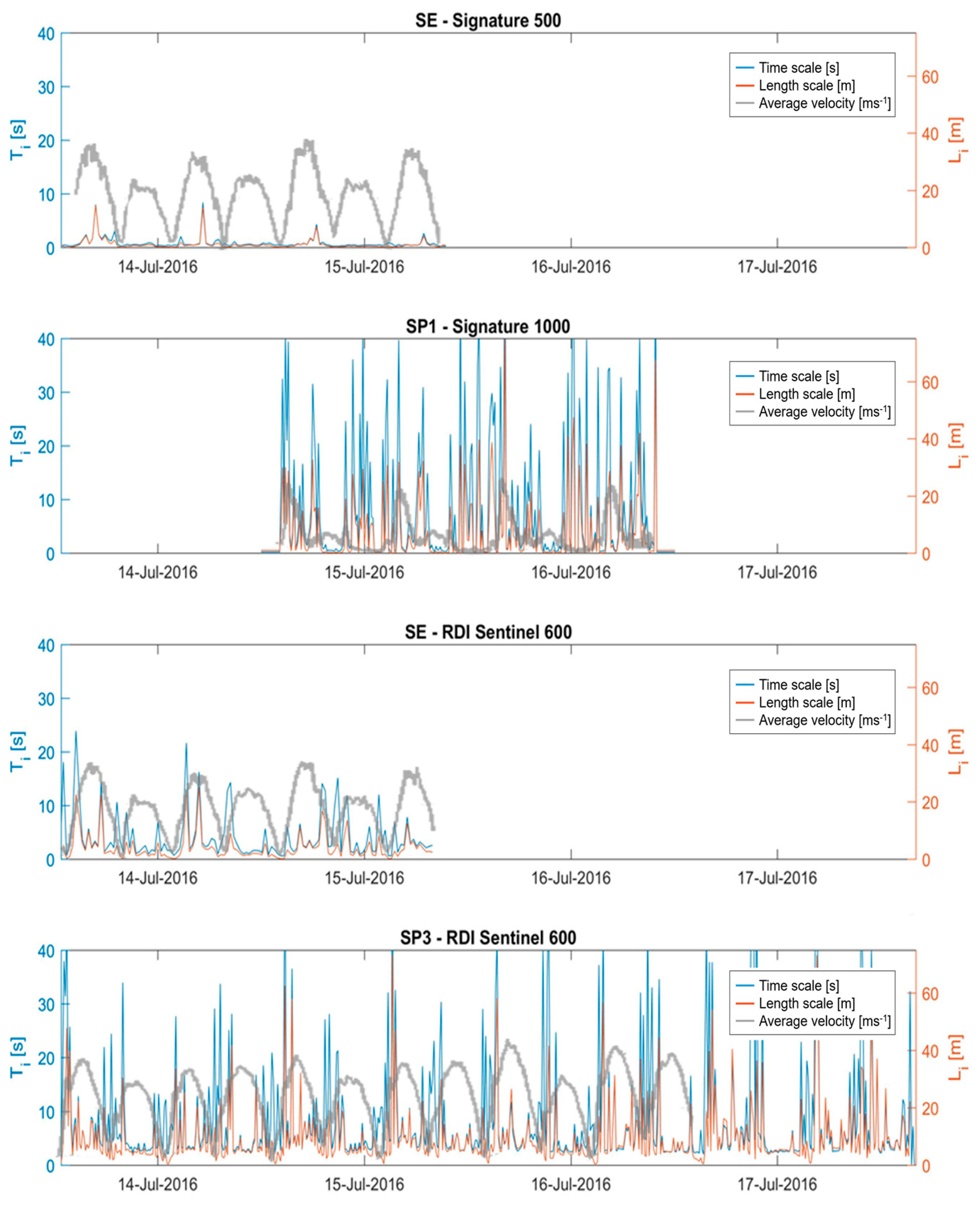
This study has highlighted the difference between the two co-located SE Signature 500 and Sentinel V50 sensors. These sensors were deployed at less than 1 m distance from each other within the same sensor frame. It was expected that the flow speeds and turbulence parameters for these sensors would record almost identical results. However, this was not the case. While exact sensor setup and sampling regime would provide a more robust comparison, the setups used were within reasonable tolerances conducive to turbulence measurements. These results should yield largely similar outcomes, where only the very high frequency turbulence components would differ. The sensor manufacturers, Nortek and Teledyne, were contacted in regards to data quality and measurement validation. This concluded that both SE located datasets were confirmed as credible data sources, with no significant defects or errors. Both hardware and firmware of both ADCPs has also been confirmed as healthy. Further comparison of the co-located sensor’s raw data, showed the presence of the variations in flow profile features, as shown in Figure 4, in the streamwise orientated beam data. This suggests these differences in measurements are a result of the sensors. This measurement campaign does not provide an explanation of the cause of this variation, but brings them to the reader’s attention. Further explanation and validation of these measurement variations, e.g., by an attempt to repeat the deployments, is limited due to the nature and cost of field measurements. Additional experimental work would benefit from collecting turbulence measurements in a laboratory flow tank, where more variables can be controlled.

The analysis of the results show the RDI Sentinel sensor having a much smoother velocity profile across the water column, whereas the Signature 500 experiences a much higher velocity variation. The data used in this study purposely extracted the sensor information in its rawest beam velocities format. This seems to be the case for the Signature 500 sensor, whereas the smooth profile of the RDI Sentinel 600 suggests that some form of internal data filtering has occurred. However, this was dismissed when contact was made with the manufacturer. When the average flow conditions are plotted, this initially assumed data cleaning shows very little effect. However, during the turbulence analysis, this apparent smoothing of the velocity variation causes significant effects to the turbulence parameters. A more direct comparison should be carried out, where the sensors sample rate and bin sizes remain constant and the sampling regime remains as similar as possible, with both sensor head aligned in the same orientation, so a direct beam-by-beam comparison is possible. However, the sampling regime will have to remain staggered to avoid sensor crosstalk. Based on the results presented and discussed in the above sections, it is recommended that a standard procedure is applied to the very basic data processing for the output of raw data for all sensor manufactures. This would require a classification of “raw data” that only allows very basic quality controls parameters to be applied. This would allow a reliable use of combined sensor types for turbulence quantification.

The results from the spatially distributed sensors all show turbulence levels that are consistent with previous literature with similar flow speeds for tidal energy test sites [11,15,19,34], where turbulence intensities are of the order of 0.1 for hub height water depths. This is with exception to the SP1 sensor, where a much more turbulent flow is shown due to wake effects from the southern point of Eday. This sensor experiences a very disrupted tidal flow pattern, where flow speeds during the ebb and later part of the flood tide are significantly reduced. This shows the spatial variability of the flow field, where large difference in flow and turbulence characteristics occur over a short distance. Based on these measurements it seems likely that a tidal device could operate without detriment as a result of turbulence, at the SE and SP3 locations. The SP3 sensor experiences significant turbulence and flow disruptions making it a poor location for turbine siting.

Further work should include longer term continuous turbulence measurements, where full spring, neap cycles are measured. Additional considerations may wish to address the impact of seasonality on turbulence characteristics, where winter storms bring large waves to exposed tidal sites, causing alteration to the turbulence depth profile.

5. Conclusions

This study investigates the spatial and temporal differences in turbulence in the southern entry to the Fall of Warness tidal energy test site in Orkney. Four high-resolution bottom-mounted diverging beam ADCPs were deployed to simultaneously collect flow characteristics for several nearby locations. The measurements were made on a waxing lunar phase, with tides midway between neaps and springs. The flow characteristics show an asymmetric velocity distribution, where maximum flood velocities of 2 ms⁻¹ at 150° and ebb velocities of 1.2 ms⁻¹ at 315° are present within the channel. The SP1 sensor, close to the easterly landmass in Figure 1, experiences flow interference midway through the flood tide that persists into the ebb tide, this provides much lower velocities with a wider directional variation.

The comparison of data from two sensors deployed in the multi-carrier frame at the same location provides different flow results and therefore different turbulence parameters. This provides uncertainty in the accuracy of turbulence measurements using ADCPs. Further comparisons between sensors should be tested in a more controlled environment, e.g., laboratory condition to identify the origins of these variations.

Several turbulence metrics are presented, where the variation in the velocity fluctuations are assessed in depth and time. The turbulence intensities show higher values towards the seabed, relative to the local velocities. The SP1 sensor shows large levels of turbulence near the surface for the flood tide and mid-water column for the ebb tide. This is supported by the presentation of the streamwise (uw) and transverse (vw) Reynold stresses. These stresses indicate larger vertical movement of turbulence in the transverse direction as opposed to the streamwise component; which generally increases towards the seabed. The time and length integral scales show longer and larger turbulent structures during the flood tides. These larger structures are located towards the seabed for the SP1 sensor, whereas for the SP3 sensor these structures are shown nearer the surface. The streamwise and beam length scales were compared at a likely depth of a turbine hub height. This showed that while the streamwise homogenous approximation should prevent the measurement of small (<10 m) length scales, the direct comparison of the individual beam data shows a similar agreement in the results. This shows similar magnitudes length scales across the flood and ebb tide, with some discrepancies occurring, where individual beam data provide larger values and higher frequency of fluctuations. The variation in turbulence between the deployment locations indicates that turbulence values can vary highly over relatively small distances. In order to quantify turbulence for a tidal energy test site for multiple numbers of devices, the deployment of several spatially distributed ADCPs must be required. Caution should be exercised when applying these turbulence conditions to other tidal energy test sites.

Further work focusses on extended deployment durations in obtaining high-resolution datasets. These extended measurement periods will provide more data to allow a more robust quantification of the turbulence parameters for an individual site. The presence of surface gravity waves will also be investigated as well as the application of the fifth vertical beam.

References

1. Blackmore, T.; Myers, L.E.; Bahaj, A.S. Effects of turbulence on tidal turbines: Implications to performance, blade loads, and condition monitoring. Int. J. Mar. Energy 2016, 14, 1–26. [Google Scholar] [CrossRef] [Green Version]
2. Milne, I.A.A.; Day, A.H.H.; Sharma, R.N.N.; Flay, R.G.J. The characterisation of the hydrodynamic loads on tidal turbines due to turbulence. Renew. Sustain. Energy Rev. 2016, 56, 851–864. [Google Scholar] [CrossRef] [Green Version]
3. Deacon, E.L. The Measurement of Turbulent Transfer in the Lower Atmosphere. Adv. Geophys. 1959, 6, 211–228. [Google Scholar]
4. Huntley, D.A. A Modified Inertial Dissipation Method for Estimating Seabed Stresses at Low Reynolds Numbers, with Application to Wave/Current Boundary Layer Measurements. J. Phys. Oceanogr. 1988, 18, 339–346. [Google Scholar] [CrossRef] [Green Version]
5. Sellar, B.; Harding, S.; Richmond, M. High-resolution velocimetry in energetic tidal currents using a convergent-beam acoustic Doppler profiler. Meas. Sci. Technol. 2015, 26, 085801. [Google Scholar] [CrossRef] [Green Version]
6. Teledyne RDI. Sentinel V—Next Gen ADCP; Teledyne RDI: La Gaude, France, 2015. [Google Scholar]
7. Nortek Signature 1000/500—A High Performance Scientific Powerhouse; Vangkroken: Bærum, Norway, 2015.
8. Lu, Y.; Lueck, R.G. Using a Broadband ADCP in a Tidal Channel. Part II: Turbulence. J. Atmos. Ocean. Technol. 1999. [Google Scholar] [CrossRef]
9. Lohrmann, A. Introduction to AD2CP Turbulence Measurements—YouTube. Available online: https://www.youtube.com/watch?v=_WyTY4N7IvY&t=581s (accessed on 30 March 2018).
10. Thomson, J.; Polagye, B.; Durgesh, V.; Richmond, M.C. Measurements of Turbulence at Two Tidal Energy Sites in Puget Sound, WA. IEEE J. Ocean. Eng. 2012, 37, 363–374. [Google Scholar] [CrossRef]
11. Thomson, J.; Polagye, B.; Richmond, M.; Durgesh, V. Quantifying Turbulence for Tidal Power Applications.
12. Richard, J.-B.; Thomson, J.; Polagye, B.; Barda, J. Method for identification of Doppler noise levels in turbulent flow measurements dedicated to tidal energy. Int. J. Mar. Energy 2013, 3–4, 52–64. [Google Scholar] [CrossRef]
13. Durgesh, V.; Thomson, J.; Richmond, M.C.; Polagye, B.L. Noise correction of turbulent spectra obtained from acoustic doppler velocimeters. Flow Meas. Instrum. 2014, 37, 29–41. [Google Scholar] [CrossRef]
14. Osalusi, E.; Side, J.; Harris, R. Structure of turbulent flow in EMEC’s tidal energy test site. Int. Commun. Heat Mass Transf. 2009, 36, 422–431. [Google Scholar] [CrossRef]
15. Milne, I.A.; Sharma, R.N.; Flay, R.G.J.; Bickerton, S. Characteristics of the turbulence in the flow at a tidal stream power site. Philos. Trans. A Math. Phys. Eng. Sci. 2013, 371, 20120196. [Google Scholar] [CrossRef] [PubMed]
16. Bouferrouk, A.; Hardwick, J.P.; Colucci, A.M.; Johanning, L. Quantifying turbulence from field measurements at a mixed low tidal energy site. Renew. Energy 2016, 87, 478–492. [Google Scholar] [CrossRef] [Green Version]
17. Milne, I.A.; Sharma, R.N.; Flay, R.G.J. The structure of turbulence in a rapid tidal flow. Proc. R. Soc. A Math. Phys. Eng. Sci. 2017, 473, 20170295. [Google Scholar] [CrossRef] [PubMed]
18. Sellar, B.; Wakelam, G.; Sutherland, D.; Ingram, D.; Venugopal, V. Characterisation of Tidal Flows at the European Marine Energy Centre in the Absence of Ocean Waves. Energies 2018, 11, 176. [Google Scholar] [CrossRef]
19. Guerra, M.; Thomson, J.; Guerra, M.; Thomson, J. Turbulence Measurements from Five-Beam Acoustic Doppler Current Profilers. J. Atmos. Ocean. Technol. 2017, 34, 1267–1284. [Google Scholar] [CrossRef]
20. McMillan, J.M.; Hay, A.E.; Lueck, R.G.; Wolk, F.; McMillan, J.M.; Hay, A.E.; Lueck, R.G.; Wolk, F. Rates of Dissipation of Turbulent Kinetic Energy in a High Reynolds Number Tidal Channel. J. Atmos. Ocean. Technol. 2016, 33, 817–837. [Google Scholar] [CrossRef]
21. Zippel, S.F.; Thomson, J.; Farquharson, G. Turbulence from Breaking Surface Waves at a River Mouth. J. Phys. Oceanogr. 2018, 48, 435–453. [Google Scholar] [CrossRef] [Green Version]
22. Konsoer, K.M.; Rhoads, B.L. Spatial–temporal structure of mixing interface turbulence at two large river confluences. Environ. Fluid Mech. 2014, 14, 1043–1070. [Google Scholar] [CrossRef]
23. Muste, M.; Yu, K.; Pratt, T.; Abraham, D. Practical aspects of ADCP data use for quantification of mean river flow characteristics; Part II: Fixed-vessel measurements. Flow Meas. Instrum. 2004, 15, 17–28. [Google Scholar] [CrossRef]
24. Horwitz, R.M.; Hay, A.E. Turbulence dissipation rates from horizontal velocity profiles at mid-depth in fast tidal flows. Renew. Energy 2017, 114, 283–296. [Google Scholar] [CrossRef]
25. GL Garrad Hassan Tidal Bladed Multibody Dynamics User Manual 2010; Garrad Hassan and Partners: Bristol, UK, 2010.
26. UK Hydrographic Office INSPIRE portal and MEDIN Bathymetry Data Archive Centre. Available online: https://www.gov.uk/guidance/inspire-portal-and-medin-bathymetry-data-archive-centre (accessed on 2 April 2018).
27. Greenwood, C.; Vögler, A.; Morrison, J.; Murray, A. Spatial Velocity Measurements using X-Band Radar at a High Energy Tidal Test Site. In Proceedings of the European Wave and Tidal Energy Conferences, Cork, Ireland, 30 July 2017. [Google Scholar]
28. Nortek How Is a Coordinate Transformation Done? Available online: https://www.nortekgroup.com/faq/how-is-a-coordinate-transformation-done (accessed on 29 March 2018).
29. Teledyne RDI ADCP Coordinate Transformation: Formulas and Calculations; Teledyne RD Instruments: Poway, CA, USA, 2008.
30. Kolmogorov, A.N. Dissipation of Energy in the Locally Isotropic Turbulence. Proc. Math. Phys. Sci. 1991, 434, 15–17. [Google Scholar] [CrossRef]
31. British Standards Institute. Marine Energy—Wave, Tidal and Other Water Current Converters Part 201: Tidal Energy Resource Assessment and Characterization; International Electrotechnical Commission: Geneva, Switzerland, 2015. [Google Scholar]
32. Kolmogorov, A.N. The Local Structure of Turbulence in Incompressible Viscous Fluid for Very Large Reynolds’ Numbers. Dokl. Akad. Nauk SSSR 1941, 30, 301–305. [Google Scholar] [CrossRef]
33. Kaneda, Y.; Ishihara, T.; Yokokawa, M.; Itakura, K.; Uno, A. Energy dissipation rate and energy spectrum in high resolution direct numerical simulations of turbulence in a periodic box. Phys. Fluids 2003, 15, L21–L24. [Google Scholar] [CrossRef]
34. Coles, D.; Greenwood, C.; Vogler, A.; Walsh, T.; Taaffe, D. Assessment of the turbulent flow upstream of the Meygen Phase 1a tidal stream turbines. In Proceedings of the Asian Wave and Tidal Energy Conference, Taipei, Taiwan, 9–13 September 2018. [Google Scholar]
Figure 1. Sensor deployment locations for the Fall of Warness measurement campaign with the bathymetry provided by UK Hydrographic Office.
Energies 12 00672 g001
Figure 2. Divergent acoustic Doppler profiler beam coordinates relative to xyz, enu and uvw.
Energies 12 00672 g002
Figure 3. Left: Average flow velocity vectors over 10 min in the streamwise coordinate system for the SE—Signature 500, SP1—Signature 1000, SE—Sentinel V50 and the SP3—Workhorse. Right: Average flow direction (degrees) and velocity (m/s) for the same sensors at a 10 min interval. With the start date time of the 13 July 2016 11:00:00 am. All data provided is taken 10 m above the seabed.
Energies 12 00672 g003
Figure 4. Average peak flood and ebb flow profiles for each sensor for three tidal phases, where blue indicates flood tide and red indicates the ebb tide. The values for the u and speed component of the ebb tide have been inverted to illustrate different flow direction.
Energies 12 00672 g004
Figure 5. Turbulence intensity. Left: I u based on 10 min windows for each sensor. Right: Turbulence intensity for the first three peak velocity flood and ebb tides, where the flood is positive (blue) and the ebb tide has been made negative (red).
Energies 12 00672 g005
Figure 6. Turbulence kinetic energy. Left: TKE based on 10 min windows for each sensor. Right: TKE for the first three peak velocity flood and ebb tides, where the flood is positive (blue) and the ebb tide negative (red).
Energies 12 00672 g006
Figure 7. Average turbulence velocity spectra for each sensor during the peak flood (blue) and ebb (red) tide at 10 m from the seabed. The individual spectra for three instances are shown in grey for each sensor during the peak flood and ebb tide. The grey dashed line is included in each subplot to indicate the −5/3 gradient of Kolmogorov’s turbulence energy cascade.
Energies 12 00672 g007
Figure 8. Reynolds stresses depth profiles for streamwise uw and transverse vw velocity components, where the flood tide is shown in blue and the ebb tide in red.
Energies 12 00672 g008
Figure 9. Integral time (blue) and length scales (red) for the streamwise velocity components. Based on measurements 20 m above the seabed for all sensors. The average velocity for each sensor is shown in grey.
Energies 12 00672 g009
Figure 10. The time (left) and length (right) integral scales presented in time and water depth for all sensors. Colour scale units are presented in seconds for the left column of subplots and meters for the right column of subplots.
Energies 12 00672 g010
Figure 11. Streamwise, beam 1 and 3 length scales, 13 m above the seabed for both SE co-located sensors. The shaded area indicates length scales shorter than the length over which the homogeneity approximation applies for the given distance from the sensor.
Energies 12 00672 g011