Initial Design Phase and Tender Designs of a Jacket Structure Converted into a Retrofitted Offshore Wind Turbine

Abstract

Jackets are the most common structures in the Adriatic Sea for extracting natural gas. These structural typologies are suitable for relative low water depths and flat sandy sea floors. Most of them have been built in the last 50 years. When the underground source finishes, these structures should be moved to another location or removed if they have reached their design life. Nevertheless, another solution might be considered: change the future working life of these platforms by involving renewable energy and transforming them into offshore wind towers. The present research proposal aims to investigate the possibility of converting actual structures for gas extraction into offshore platforms for wind turbine towers. This simplified analysis is useful for initial design phases and tender design, or generally when available information is limited. The model proposed is a new simplified tool used to study the structural analysis of the jacket structure, developed and summarized in 10 steps, firstly adopted to study the behavior of the oil and gas structure and then for the retrofitted wind tower configuration.

1. Introduction

Policy support, technology advances, and a maturing supply chain are making offshore wind farms an increasingly viable option for renewable-based electricity generation, harnessing the more consistent and higher wind speeds available offshore instead the onshore solutions. Investment has picked up sharply in recent years, and with fewer restrictions on size and height with respect to their onshore counterparts, offshore wind turbines are becoming giants [1]. The growth of offshore wind creates potential synergies with the offshore hydrocarbons sector; integration could bring benefits in terms of reduced costs and improved environmental performance and utilization of infrastructure [2,3]. The possibility to electrify offshore oil and gas operations where there are wind farms nearby, or via floating turbines, reduces the need to run diesel or gas-fired generators on the platform and emissions of carbon dioxide (CO${}_2$) and air pollutants [4]. The scope is to find new uses for existing offshore infrastructure once it reaches the end of its operational life or when the underground source finishes, in ways that might aid energy transitions [5,6]. The North Sea, a relatively mature oil and gas basin with a thriving renewable electricity industry, is already seeing some crossover between the sectors: some large oil and gas companies are major players in offshore wind; one former oil and gas company, Orsted in Denmark, has moved entirely to wind and other renewables [7,8]. A major problem in offshore wind energy design is the estimation of fatigue life and fatigue loads in an offshore environment [9,10]. The study of the best locations of offshore wind turbines is worth investigation as well [11]. However, many studies have been devoted to how the dynamic behaviors of wind turbines couple with jacket and pile-supported foundations [12,13,14,15,16,17,18,19,20,21].

This work aims to provide a tool for a general structural check analysis of a different retrofitting activities for the same offshore lattice structure. The research should allow the structural designer to evaluate the environmental loads, the dynamics of the structure, and the effects of changing the structural behavior of the platform over the different cases of study. All these analyses should be available in the early design phase when the data available about the site’s environment and seabed conditions are limited. Furthermore, the tools shown should skip the use of the sophisticated and expensive software analysis that requires detailed data and a high level of understanding of the underlying physics. It follows that the calculation procedure will be faster than the long run-times of the software, which is based on time domain simulations of a high number of different load cases. MATLAB and Strand7 have been used as software programs in this research. In terms of accuracy, the most important requirement is that the approach should provide conservative results and at the same time avoid underestimation of loads and deformations. The issue of this project is to find a useful tool that is able to represent the behavior of a generic offshore structure subjected to environmental actions. The structure under investigation can be one of the oil and gas platforms sustained by jacket structures with a long pile foundation. The authors are aware of the complex problem that is presented here. Therefore, the present research is limited, but in agreement with the assumptions considered in this study. Further investigations can be performed in a future work such as tubular joint design [22] and fatigue assessment [23,24]. The influence of a different wind turbine such as vertical axis wind turbines [25] and wind turbines in other environments [26,27] is also worth investigating.

2. Theoretical Background

Offshore structures are complex systems subjected to severe dynamic loads due to wind, waves, currents, and mechanical loads. This makes the design of these structures a complex process that requires expertise from a wide range of fields. Foundations and substructures are specifically the key structural components that differentiate the design of wind towers from those of onshore ones. Due to the long service lifetime of offshore systems, the analysis of the performance of the substructure is a complex task that involves many steps including load analysis, dynamic analysis, evaluation of the fatigue life, as well as long-term deformations. This research presents a simplified methodology for the analysis of the ultimate and dynamics loads with a check on the most stressed pile of the different offshore retrofitted systems. The analysis was carried out such that the data required about the oil and gas platform, wind turbines, and the site are available in the early design phases. Thus, the methodology appears to obtain a conservative estimation. An apparent limitation in the research is the modeling of first the oil and gas platform and second of the offshore wind turbine called 6DOF with all the retrofitting configurations, which was realized in general form, and it found adaptation in different specific applications. The model proposed considers a discrete system of masses and stiffness, which is just a first rough representation of the real offshore lattice structure with pile foundation. Another inherent limitation in the methodology, which is a natural consequence of the approach taken, is the load estimation based on linear analysis and where they are applied. In the model proposed, all the environmental actions are considered at each node of the cantilever beam, while in the real world, all the steel elements are subjected to the wave and wind force. Another issue of the loads is that in this research is that they have not been calculated using partial safety factors regarding the load combination. The present analysis is performed only over one direction with the assumption that the wind and the wave act in the same direction at the same time. Fatigue state analysis is out of the scope of the present research; nevertheless, this is central to the structural analysis, the earthquake analysis, and the checking of the state of the structure like welding, bolts, and grouting, which for sake of simplicity’s, have been bypassed. The simplified analysis proposed in this research can be used in the fatigue design and evaluation including the effects of welding, bolts, and the stiffness of tubular connections [28,29]. The next stage of the current research study will address fatigue analysis using current (global rules) and advanced approaches (local rules) for the critical structural detail considering the wave and wind loads as indicated in the DNVGLstandards.

The equation of motion associated with a generic structure is a second order linear differential equation with constant coefficients, and it changes form in relation to the structural properties that have to be modeled. The general set of equations representing structural motion can be defined by the following matrix form:

$$\mathit{M}\ddot{\mathbf{\xi }}+\mathit{C}\dot{\mathbf{\xi }}+\mathit{K}\mathbf{\xi }=\mathit{p}$$

(1)

that represents a finite set of N ordinary, linear differential equations in N independent coordinates that contain the dominant features of the structural motion. These coordinates are the elements of the column vector:

$$\mathbf{\xi }={[{\xi }_1,{\xi }_2,\dots ,{\xi }_N]}^T$$

(2)

The loading vector $\mathit{p}=\mathit{p}\left(t\right)$ is comprised of N loads $p_i$, $i=1,2,\dots ,N$ where the load $p_i=p_i\left(t\right)$ is located at the respective node i. The vector representation is:

$$\mathit{p}={[p_1,p_2,\dots ,p_n,\dots ,p_N]}^T$$

(3)

In this analysis, the mass matrix M is assumed to be a diagonal matrix with elements $m_i>0$, $i=1,2,\dots ,N$, in which the element’s subscript is its associated node point. It has been said that each generalized coordinate represents either the displacement or the rotation of a portion of the structure’s mass at a specific node point. The mass lumping method is probably the most popular method of discretizing the supporting framework and the rigid body portions of an offshore structure. In this research, the mass lumping method will be applied where all the offshore mass structure is modeled as lumped at the top of a cantilever beam. The stiffness matrix K for an N degree of freedom structure is a symmetric matrix of $N\times N$ elements. The stiffness is defined as the force applied to the structure in order to produce a unitary displacement. The constant $k_{ij}$ in other terms is that force that is required at node i to counteract a unit elastic displacement ${\xi }_{sj}=1$ imposed at node j, under the condition that all displacements ${\xi }_{si}=0$ for $i\ne j$. If a displacement condition is applied sequentially to each node, then the net force at each node j can be obtained by superposition. For a structure with N degrees of freedom, the damping matrix C is defined as a symmetric array of $N\times N$ constants $c_{ij}$. Damping is an influence within or upon an oscillatory system that has the effect of reducing, restricting, or preventing its oscillations. In physical systems, damping is the capacity of the system to dissipate the energy stored in the oscillation within itself without damage. In this analysis, the damping force $q_{Di}$ for the structural mode coordinate $\xi$ is assumed to be a linear combination of the generalized coordinate velocities ${\dot{\xi }}_i$, $i=1,2,\dots ,N$:

$${\mathbf{q}}_{\mathbf{D}}=\mathit{C}\dot{\mathbf{\xi }}$$

(4)

The damping matrix can be cast in several different specialized forms, each of which has the advantage of easily utilizing available experimental data to determine the elements $c_{ij}$. One such form is Rayleigh damping in which C is proportional to the system’s mass and also the system’s stiffness:

$$\mathit{C}=a_1\mathit{M}+a_2\mathit{K}$$

(5)

in which $a_1$ and $a_2$ are Rayleigh constants, and they are fixed for a given dynamic system. Rayleigh constants are determined using a standardized procedure [30]. The latter equation is pre- and post-multiplied by the matrix of the shape functions as ${\mathit{X}}^T\mathit{CX}=a_1{\mathit{X}}^T\mathit{KX}+a_2{\mathit{X}}^T\mathit{MX}$ with the orthogonal properties ${\mathit{X}}^T\mathit{KX}=diag\left({\omega }_n\right)$ and ${\mathit{X}}^T\mathit{MX}=\mathit{I}$. Introducing the nth modal damping factor ${\zeta }_n$, the last result becomes ${\mathit{X}}^T\mathit{CX}=diag(a_1{\omega }_n^2+a_2)=diag\left(2{\zeta }_n{\omega }_n\right)$. After equating the nth diagonal terms above, it follows that ${\zeta }_n=({\omega }_n/2)a_1+\left(0.5{\omega }_n\right)a_2$. This last result shows that, for an N degree of freedom system for which the N frequencies ${\omega }_1,{\omega }_2,\cdots ,{\omega }_N$ are known, the two Rayleigh constants $a_1$ and $a_2$ are uniquely determined if any two of ${\zeta }_n$ are specified. For instance, if ${\zeta }_k$ and ${\zeta }_m$ are specified, then the equation yields the following two simultaneous equations from which $a_1$ and $a_2$ can be calculated ${\zeta }_k=({\omega }_k/2)a_1+\left(0.5{\omega }_k\right)a_2$ and ${\zeta }_m=({\omega }_m/2)a_1+\left(0.5{\omega }_m\right)a_2$. Then, the remaining $N-2$ values of ${\zeta }_n$ for all $n\ne m$ can be determined.

3. Reference Model

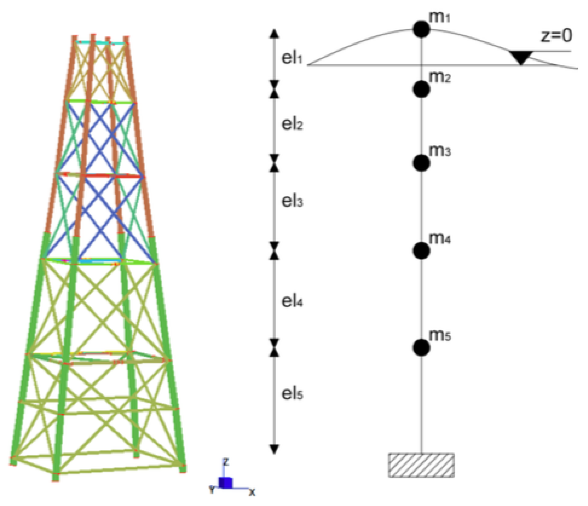
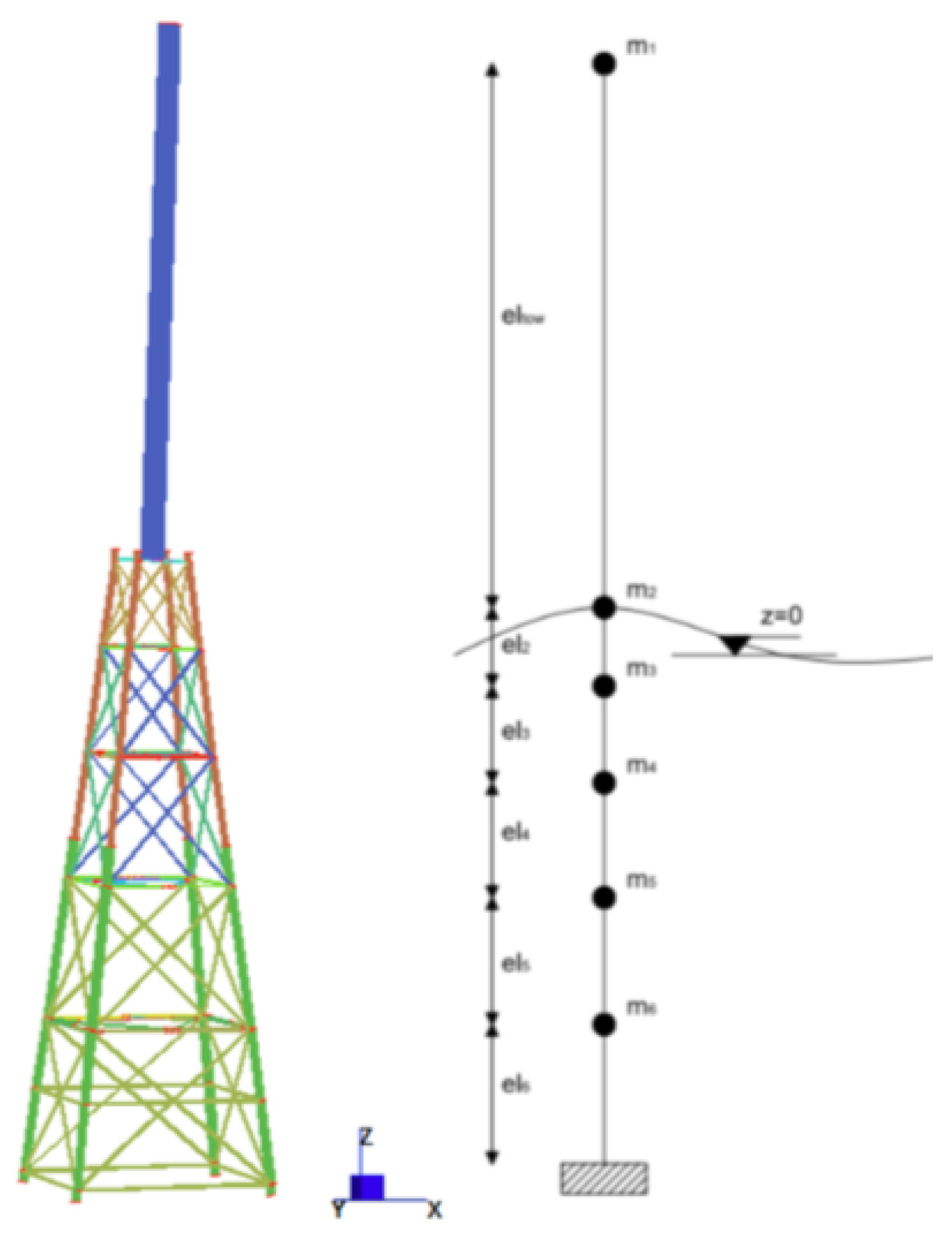
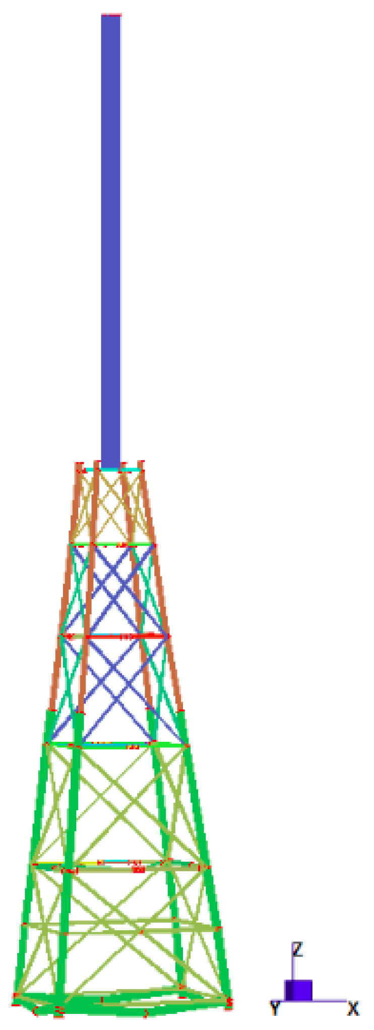
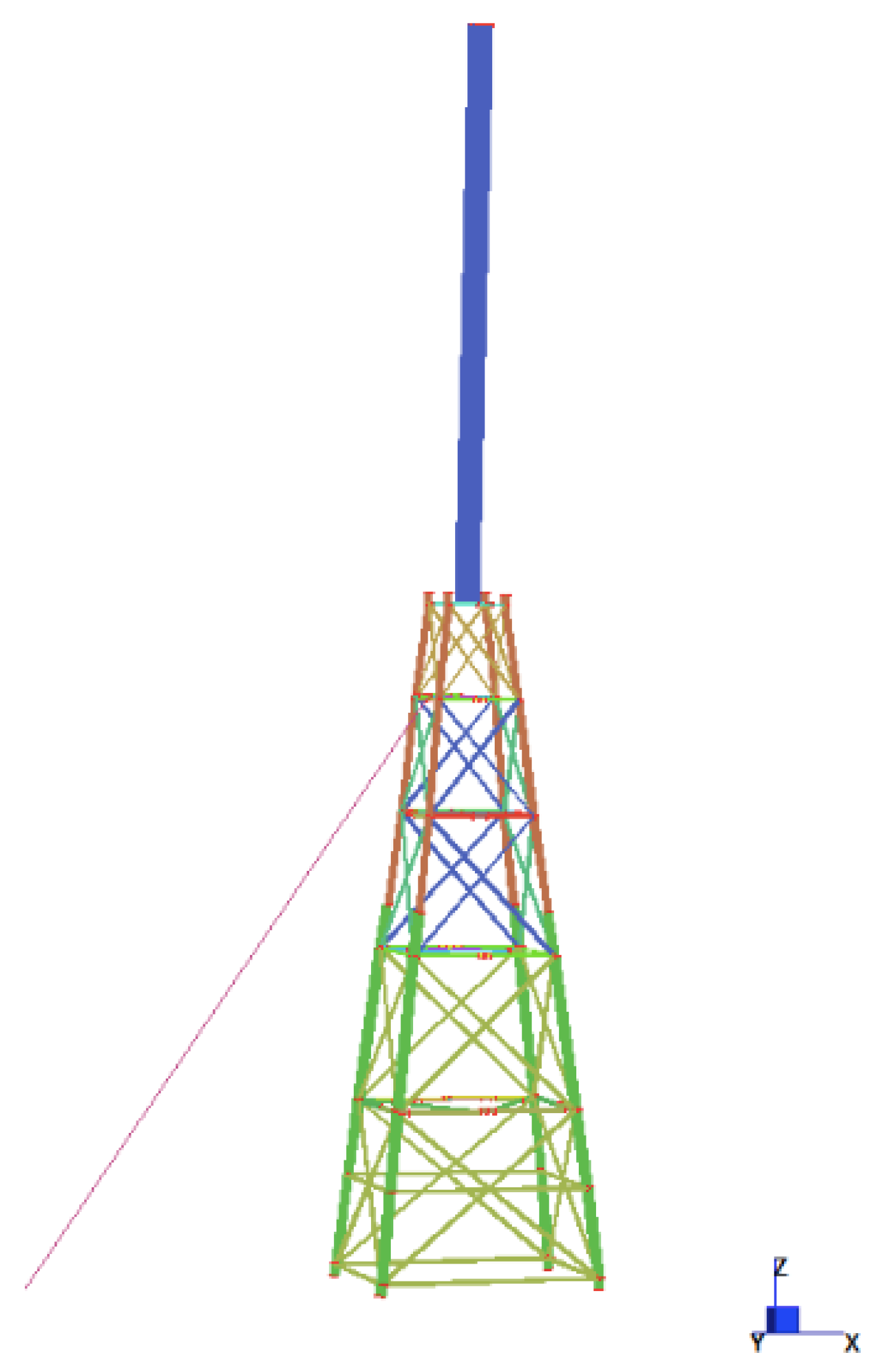
Let us suppose that the oil and gas platform studied in this detection is part of a wide context of a gas field, in a water depth of 87 m. The platform sub-structure is a steel jacket, installed by lifting, supporting a three generic level deck for the drilling and extraction activities. The jacket configuration is represented by a four-legged tubular structure, and the jacket base dimensions are approximately 32 m by 20 m (excluding the sleeves). The jacket dimensions at the top interface are 8 m × 8 m. Jacket planes are located at the following elevations from top the bottom with respect to the still water level: +6 m, −8.5 m, −24.5 m, −43.5 m, −64.5 m. The leg diameter varies from 1200 mm by 40 mm at the top to 1600 mm by 50 mm at the bottom. For the bracing elements, the diameter varies from 600 mm by 10 mm–800 mm by 15 mm. Figure 1 is a possible representation of the jacket substructure, the subject of this analysis, realized using Strand7 and MATLAB software.

All analysis steps necessary for the simplified design of an offshore structure have been done introducing a 10-step modeling approach:

• Structural and environmental parameters
• Undamped motion of the structure
• Damped frequencies’ definition
• Response to environmental loads
• Maximum load pile applied
• Time domain solution
• Transfer function definition
• Spectral density function of the generic load
• Response spectrum
• $3\sigma$ approach

In order to test if the activity model conforms to the real response of the structure, two methods of analysis will be tested for the same structure. One has been developed using MATLAB software and the other one using the Strand7 software. If the results are coherent, the modeling could be said to be efficient and suitable for the representation of the behavior of a generic jacket steel structure.

Platform properties and environmental parameters are described below. The steel jacket is modeled with five lumped masses placed at different heights, one at each horizontal plane and clamped at the bottom. The generic lumped mass is the sum of all the tubular masses surrounding the center of the horizontal plane, in particular half above and half below the generic horizontal plane. A real complex steel jacket structure can be studied using an FE model in Strand7. All the masses have been calculated considering the specific weight of steel 7850 kg/m${}^3$ multiplied by the generic cross-section and multiplied by the length of the tubular members. The diagonal mass matrix M of the 5DOF model expressed in kg developed in MATLAB:

$$\begin{array}{c}\hfill \mathit{M}=\left[\begin{array}{ccccc}{m}_1& 0& 0& 0& 0\\ 0& m_2& 0& 0& 0\\ 0& 0& m_3& 0& 0\\ 0& 0& 0& m_4& 0\\ 0& 0& 0& 0& m_5\end{array}\right]=\mathrm{diag}\left[\mathrm{581,889},\mathrm{122,432},\mathrm{147,074},\mathrm{242,301},\mathrm{206,739}\right]\end{array}$$

(6)

The stiffness matrix K has been determined along the direction x. Once having applied the definition of stiffness to all the system, it is possible to define (using MATLAB) the matrix K in N/m as:

$$\begin{array}{c}\hfill \mathit{K}=\left[\begin{array}{ccccc}{k}_{11}& k_{21}& k_{31}& k_{41}& k_{51}\\ k_{12}& k_{22}& k_{32}& k_{42}& k_{52}\\ k_{13}& k_{23}& k_{33}& k_{43}& k_{53}\\ k_{14}& k_{24}& k_{34}& k_{44}& k_{54}\\ k_{15}& k_{25}& k_{35}& k_{45}& k_{55}\end{array}\right]=\left[\begin{array}{ccccc}0.6568& -0.6568& 0& 0& 0\\ -0.6568& 1.1290& -0.4722& 0& 0\\ 0& -0.4722& 0.9560& -0.4838& 0\\ 0& 0& -0.4838& 1.0523& -0.5685\\ 0& 0& 0& -0.5685& 1.0390\end{array}\right]·{10}^9\end{array}$$

(7)

The sea state analysis has been simplified, and sample values have been chosen through Pierson–Moskowitz spectra. Such a distribution is an empirical equation for deep water waves that defines how the energy is distributed with respect to the wave frequency. It is based on the assumption of the fully-developed sea in which the wind blows constantly for a long time over an unlimited fetch area. Another wave spectrum (termed JONSWAP) might be taken into account. It is typical of the North Sea characterized by a limited fetch area. The aim of this project is not to reproduce a specific study of a particular case, but to find a generic tool to reproduce an easier and faster way expressed in terms of analysis cost of the dynamic behavior of a generic lattice structure. The quality of this model is also promoted by the flexibility, the adaptability of the frame, which represents a valid approach to consider different cases. The reader is free to reproduce the analysis using the JONSWAP spectra.

These data characterize the definition of the wave loads defined by Morison’s equation against the structure. The following sea state conditions have been chosen as wave height $H=11.6$ m, the wave period $T=12$ s, the wavelength $\lambda =1.56T^2$ = 226 m, the wave frequency $\omega =2\pi /T=0.5236$ rad/s, and the salt water density $\rho =1031$ kg/m${}^3$.

The free undamped motion of the structure is investigated solving the eigenvalue problem:

$$\det (\mathit{K}-{\omega }^2\mathit{M})=0$$

(8)

Thus, the five undamped natural structural frequencies for free vibration in rad/s of the 5DOF model in rad/s are:

$$\begin{array}{c}\hfill {\omega }_1=11.4498,{\omega }_2=35.8886,{\omega }_3=68.9503,{\omega }_4=87.9880,{\omega }_5=110.9217\end{array}$$

(9)

Modal shape matrix X is also identified for each natural structural frequency ${\omega }_n$. Each modal vector is identified by ${\widehat{\mathbf{\xi }}}_{\mathit{n}}={[{\widehat{\xi }}_{1n},{\widehat{\xi }}_{2n},\dots ,{\widehat{\xi }}_{Nn}]}^T={[1,{\widehat{\xi }}_{2n},\dots ,{\widehat{\xi }}_{Nn}]}^T$. Those vectors are normalized with respect to the mass matrix to form the new modal vectors ${\mathit{x}}_{\mathit{n}}={\widehat{\xi }}_{\mathit{n}}/e_n$, where $e_n$ is a set of positive and real constants computed from ${\widehat{\mathbf{\xi }}}_{\mathit{n}}^{\mathit{T}}\mathit{M}{\widehat{\mathbf{\xi }}}_{\mathit{n}}=e_n^2$. It follows that the modal shape matrix X of the 5DOF model is defined as the assembly of the normalized modal vectors ${\mathit{x}}_{\mathit{n}}$:

$$\begin{array}{c}\hfill \mathit{X}=[{\mathit{x}}_{\mathbf{1}},{\mathit{x}}_{\mathbf{2}},\dots ,{\mathit{x}}_{\mathbf{5}}]=\left[\begin{array}{ccccc}1.1& 0.6& 0.3& -0.2& 0.2\\ 1.0& -0.1& -1.0& 1.1& -2.2\\ 0.8& -0.9& -1.7& 0.7& 1.5\\ 0.5& -1.4& 0.1& -1.3& -0.4\\ 0.3& -1.0& 1.4& 1.3& 0.2\end{array}\right]·{10}^{-3}\end{array}$$

(10)

Associated with five undamped natural structural frequencies for free vibration ${\omega }_n$ with $n=1,2,\dots ,5$ are the five corresponding vibration modes of the 5DOF model.

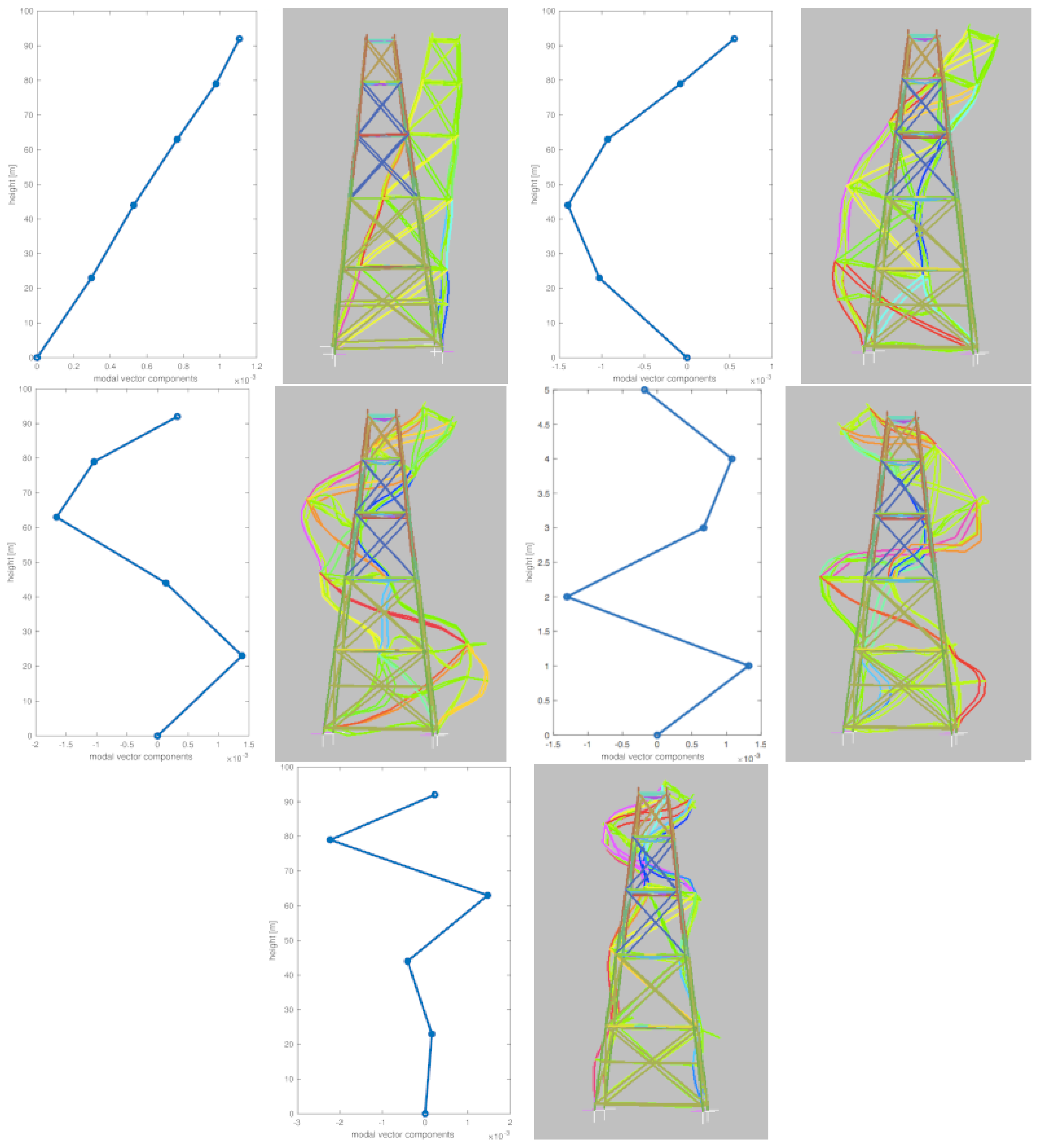
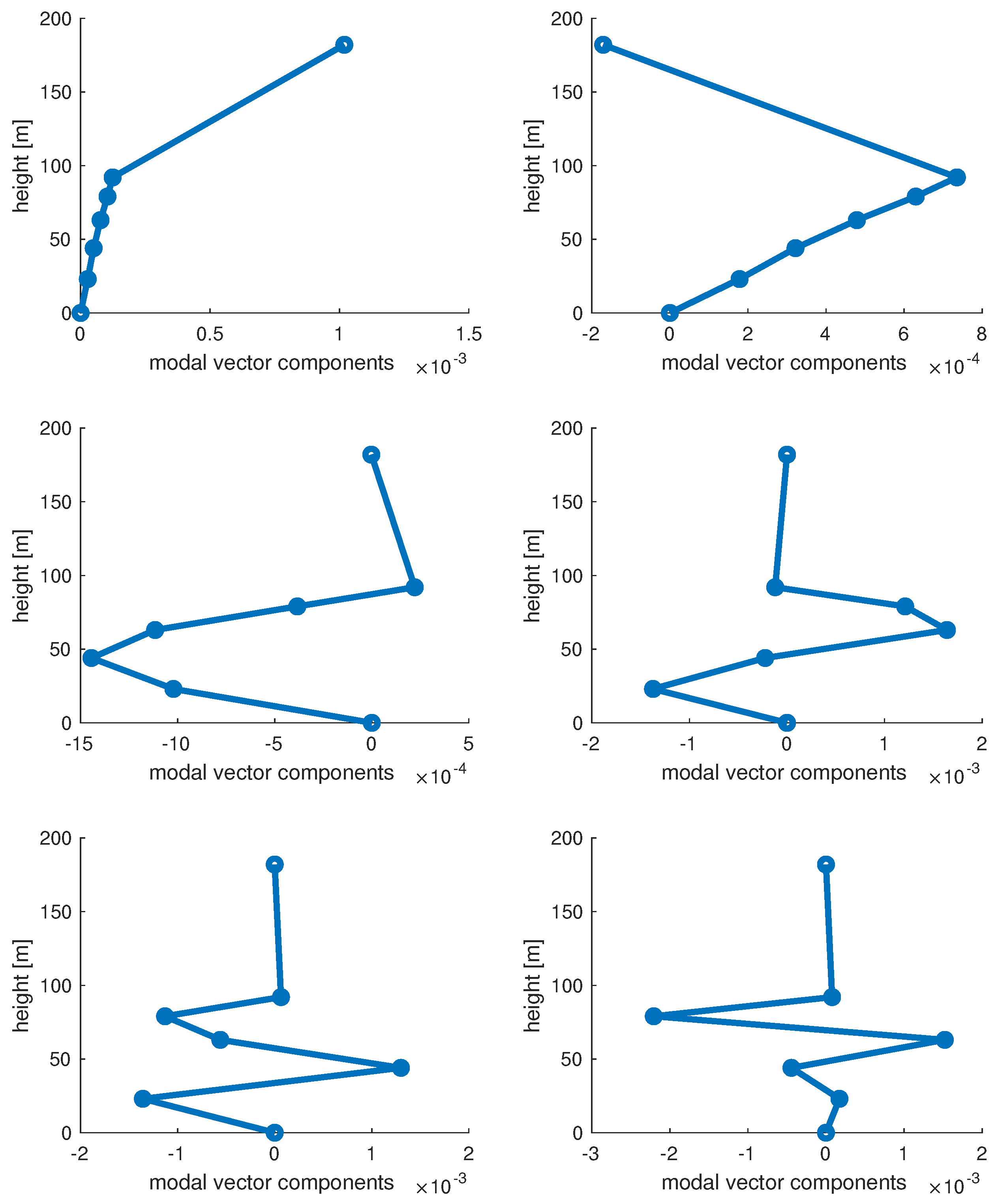
A benchmark test with Strand7 software is carried out for verification purposes using natural frequency analysis. Forty vibration modes have been considered, because the FE model is made of several 1D beam elements. The five vibration modes given by the MATLAB code are compared to the ones obtained via FE in Figure 2. The undamped natural frequencies in rad/s are: ${\omega }_1=14.33$, ${\omega }_2=35.00$, ${\omega }_3=57.93$, ${\omega }_4=76.97$, and ${\omega }_5=104.62$.

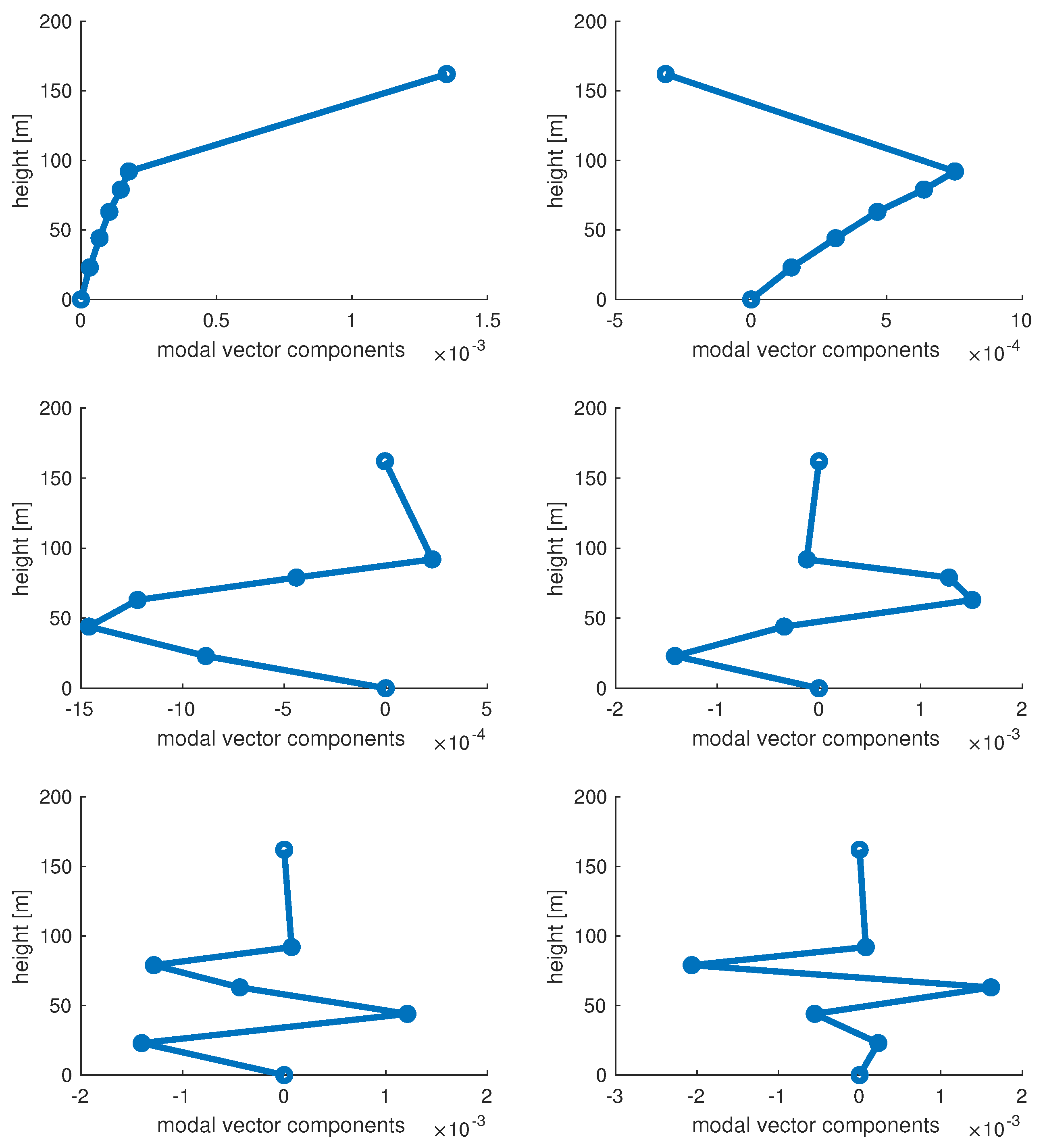
It can be noted that the mode shapes obtained by MATLAB are close to the ones obtained by FE simulation, as well as the corresponding natural undamped frequencies.

Subsequently, damped natural frequencies should be computed because they better represent the structural behavior of real structures. Rayleigh damping is considered for this purpose. Damped frequencies are characterized by the two Rayleigh constants $a_1$ and $a_2$, which are uniquely determined if any two of the modal damping factors ${\zeta }_n$ are specified. Since the first few modes will dominate the motion, it is reasonable to choose ${\zeta }_1={\zeta }_2=0.05$.

Thus, the five damped natural structural frequencies for free vibration in rad/s of the 5DOF model are:

$$\begin{array}{c}\hfill {\omega }_{d1}=11.4355,{\omega }_{d2}=35.8437,{\omega }_{d3}=68.7227,{\omega }_{d4}=87.5516,{\omega }_{d5}=110.0883\end{array}$$

(11)

The fourth step, of the present procedure, regards the response of the structure to the harmonic wave. Airy theory is considered, and it is assumed that the motion of the structure is much smaller than the motion of the wave; thus, Morison’s equation can be applied. The inertia counterpart of the flow is represented through the inertia coefficient $C_M=2$, while the drag counterpart by the drag coefficient $C_D=0.8$. The structure has been modeled with four vertical legs $N_l=4$ plus two horizontal cross braces $N_c=2$, which are normal to the flow. The calculation of the wave forces follows the guidelines reported by classical books of offshore structural modeling [30]. Wave loads for the present problem in kN are:

$$\begin{array}{c}\hfill p_1=580.53,p_2=1132,p_3=1125.3p_4=1092,p_5=1111.1\end{array}$$

(12)

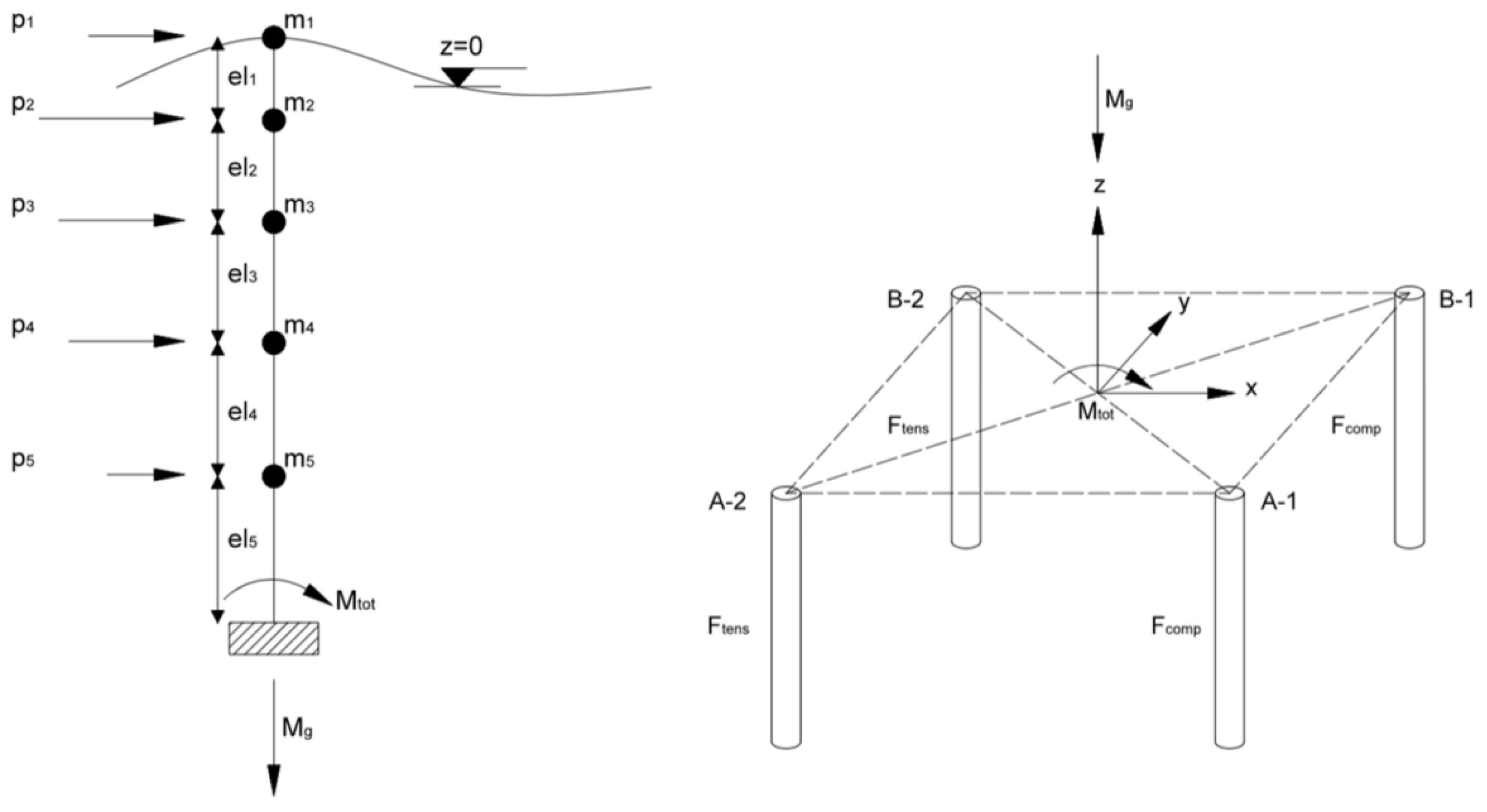
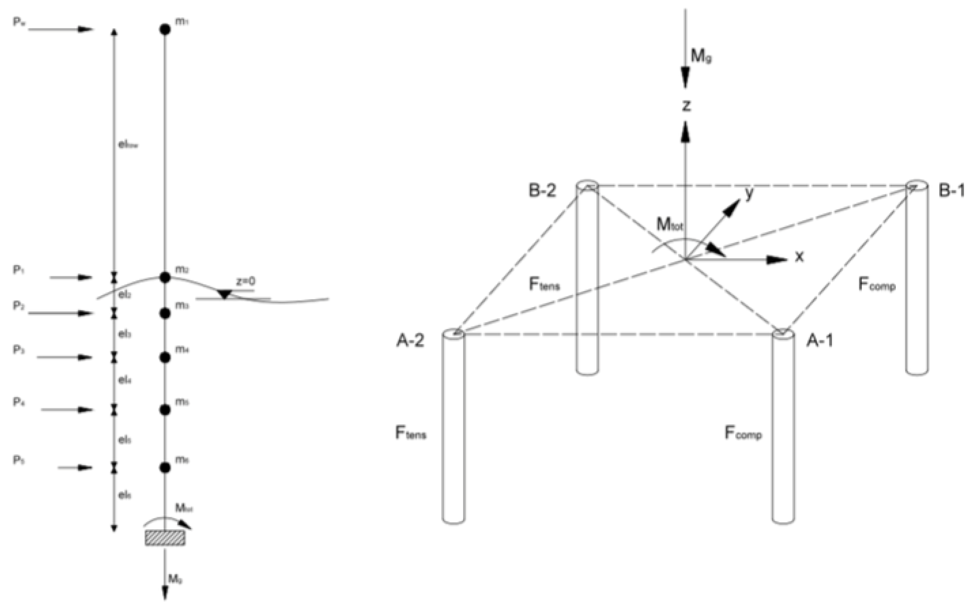
The fifth step is related to the pile stress analysis at the foundation level. Global bending moment at the foundation level is considered due to all the forces of the model. The final stress on the pile is determined by the bending moment and the weight of the structure (Figure 3).

Moreover, a wind force $F_{wind}$ = 410 kN is considered acting on the superstructure $z_{wind}$ = +7.5 m. Therefore, the force applied on the pile B-1 is $F_{B1}=-8316.28$ kN. As the numerical benchmark, the same analysis is performed in the FE model. The maximum compression value of the stress in piles given by Strand7 is in the pile B1 and is equal to $F_{B1}=-9922$ kN, while the MATLAB calculation has given $F_{B1}=-8316$ kN. There is a high correlation between the two values; indeed, they differ by only of 16%. It follows that the 5DOF model proposed in this research is working properly.

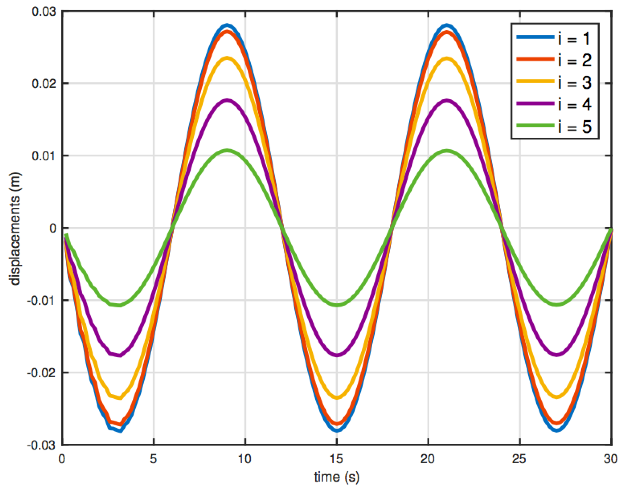
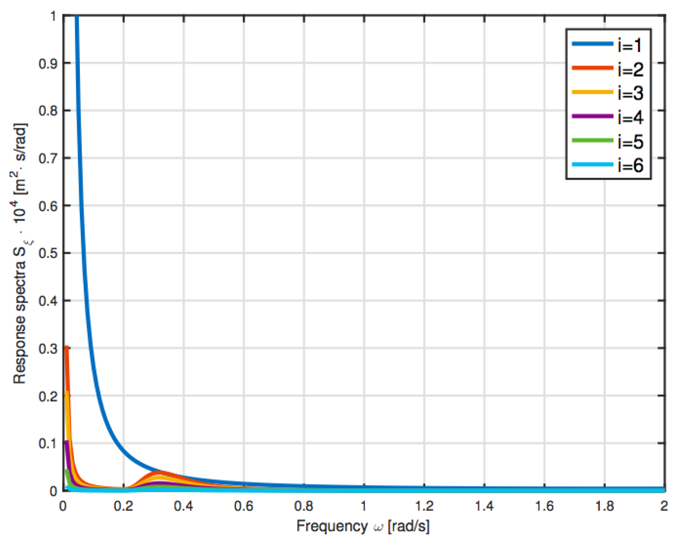
The sixth step is based on the time domain solution. These five structural steady state displacements over a time of 30 s, or in other words, the response of the structure subjected to five cycles of wave loading, are depicted in Figure 4.

The absolute value of the maximum peaks in m are: ${\xi }_1=0.02813$, ${\xi }_2=0.027214$, ${\xi }_3=0.02356$, ${\xi }_4=0.017664$, ${\xi }_5=0.01073$. These values are then compared with the results obtained with the $3\sigma$ approach that defines structural safety according to the stochastic approach. The simulation is verified via FE analysis, leading to ${\xi }_1=0.0384$, ${\xi }_2=0.0348$, ${\xi }_3=0.0278$, ${\xi }_4=0.0187$, ${\xi }_5=0.0101$.

The maximum displacements obtained with MATLAB and FE are of the same magnitude. The ratios between the displacement obtained with MATLAB and Strand7 are listed in

Table 1. Comparison between MATLAB and Straus7 displacements.

	MATLAB	FE	Ratio
${\xi }_1$	0.0281	0.0384	0.73
${\xi }_2$	0.0272	0.0348	0.78
${\xi }_3$	0.0236	0.0278	0.85
${\xi }_4$	0.0177	0.0187	0.95
${\xi }_5$	0.0107	0.0101	1.06

.

Small deviations can be observed. However, this is due to the simplifications introduced; nevertheless, as a preliminary design phase, the results can be considered worthy for proceeding in the present study. It follows that the model fully satisfies the requirements of this research.

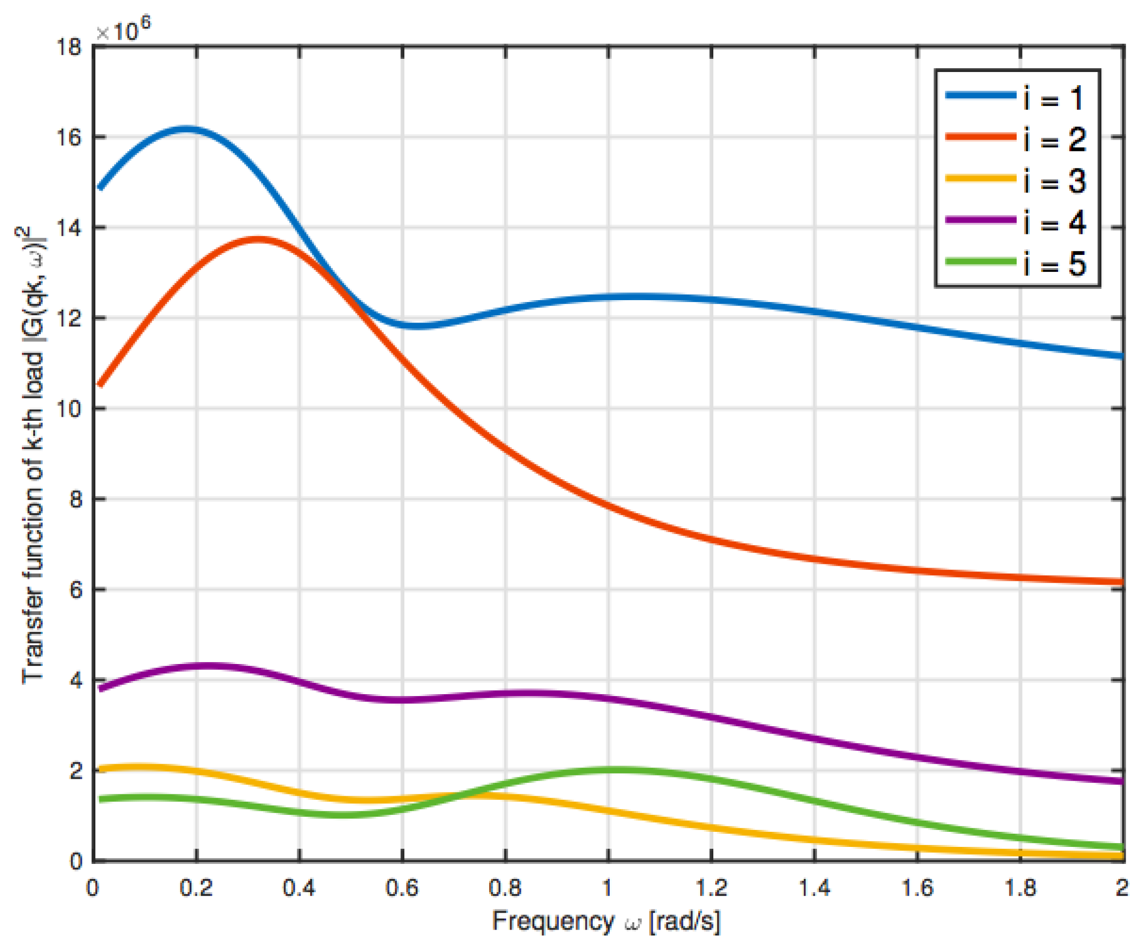
The seventh step defines the wave transfer functions for the model. The transfer function $G\left(\omega \right)$ is a function that relates the wave height H of the incident wave to the load imparted to the structural component. It is generally defined in harmonic form: $G\left(\omega \right)=G_0{e}^{j\omega t}$ with $j=\sqrt{-1}$, and $G_0$ is a complex number independent of time. The transfer function depends on the flow regimes and the structural component. Transfer functions are computed for all components and assembled for the structure. The transfer function can be applied only to linear analysis (as in the present case), and the effect of multiple wave excitation can be considered (which is not possible in the nonlinear regime). The calculation of the wave transfer function follows the indication provided in [30], and the plot of the modulus square of the five transfer functions $|{\mathit{x}}_{\mathit{k}}^{\mathit{T}}{\mathit{G}(p,\omega )|}^2={\left|G({\overline{q}}_k,\omega )\right|}^2$ is given in Figure 5.

Spectral Density Function of the Generalized Force Component in Modal Coordinates

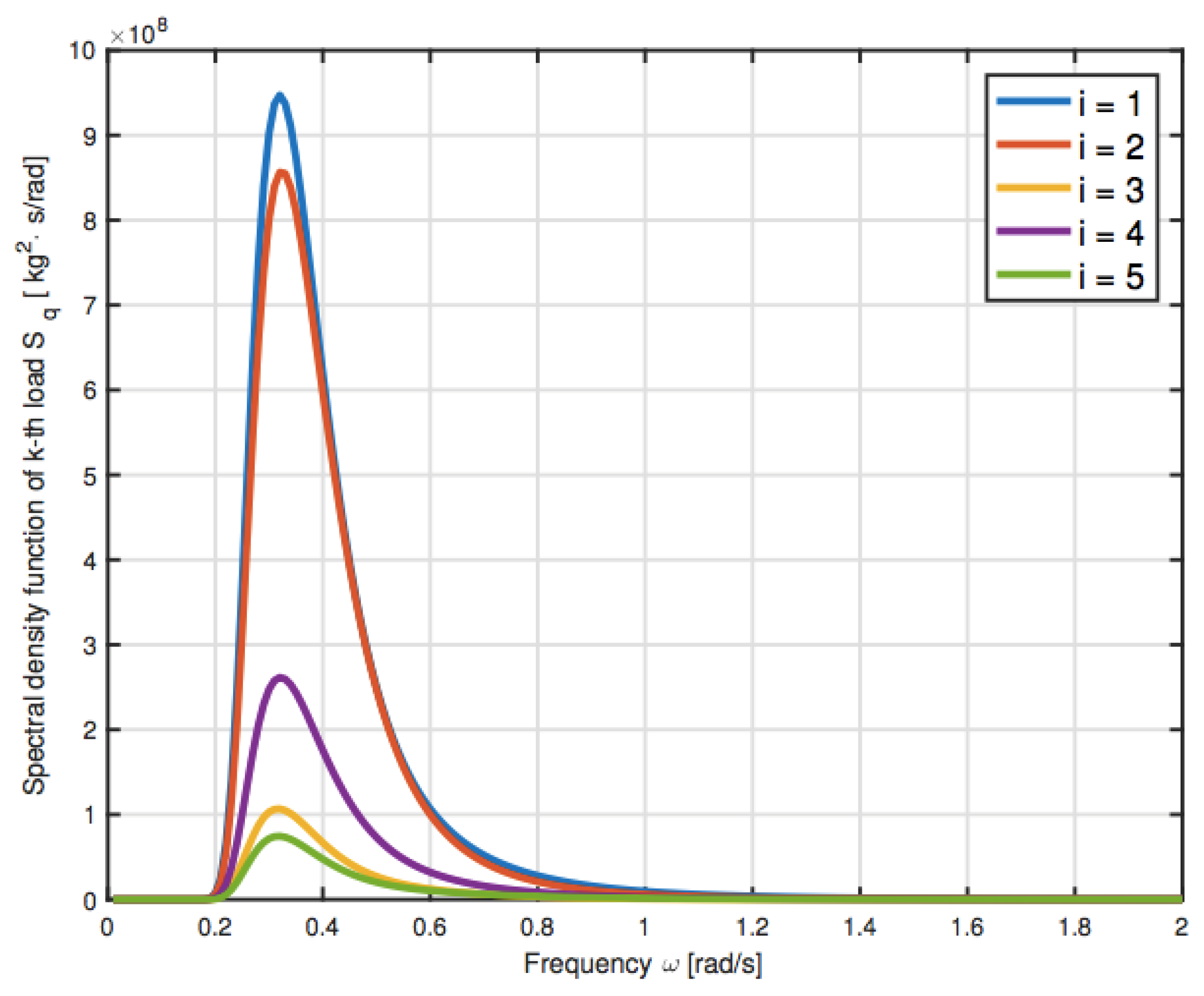
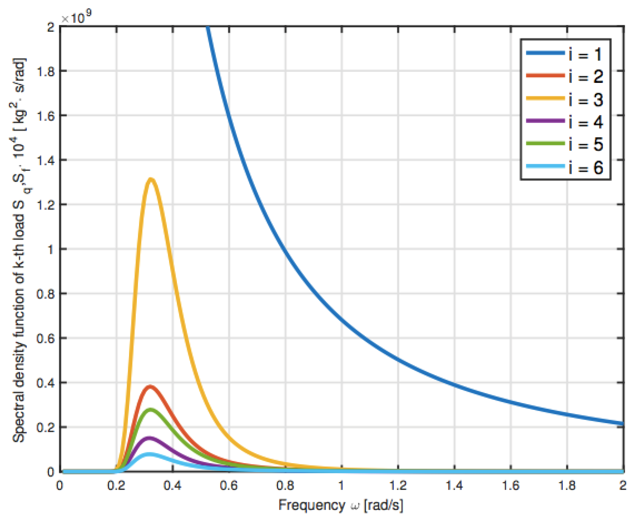
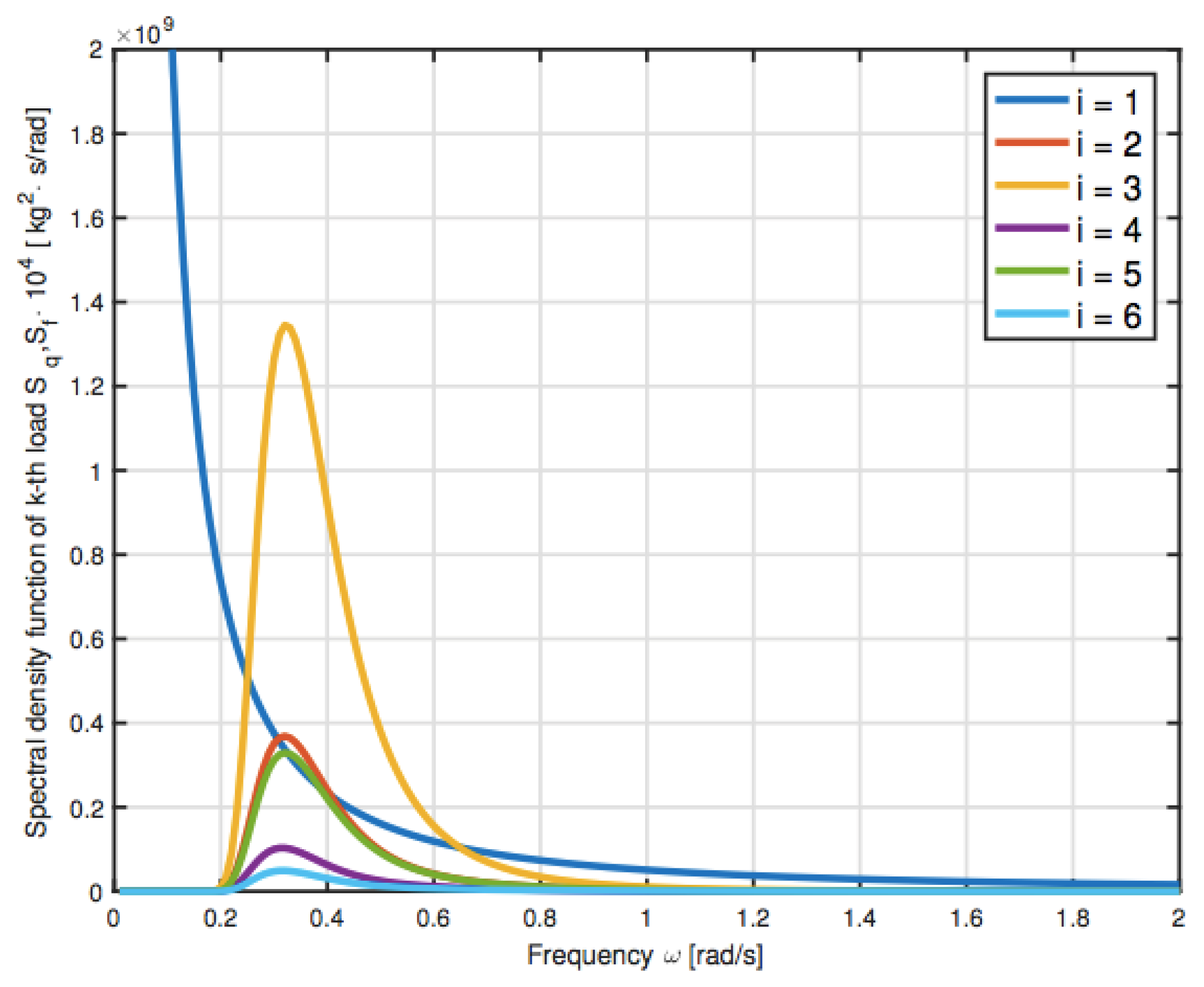
The eighth step is based on the definition of the spectral density function of the generalized force component in modal coordinates. It is necessary to determine first the Pierson–Moskowitz wave spectrum [30]:

$$S_{\eta }\left(\omega \right)=0.0081\frac{g^2}{{\omega }^5}{e}^{-B/{\omega }^4}$$

(13)

with $B=0.74{(g/V)}^4$ where v is the wind speed in m/s at a height of 19.5 m above the still water level and $\omega$ is expressed in rad/s. Multiplying the transfer function of the load in modal coordinates by the Pierson–Moskowitz spectrum, it achieved the spectral density function of the generalized force component in modal coordinates (Figure 6).

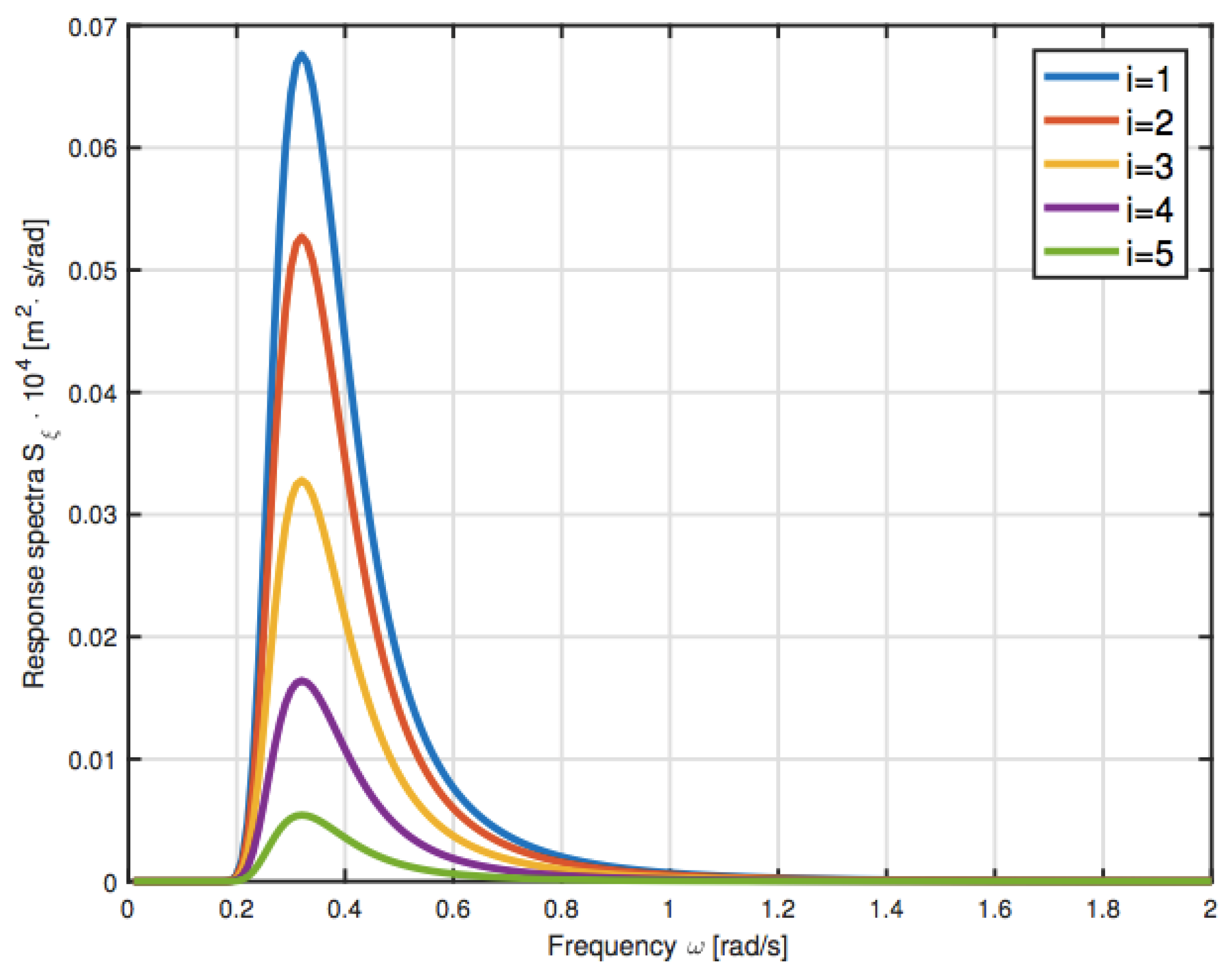
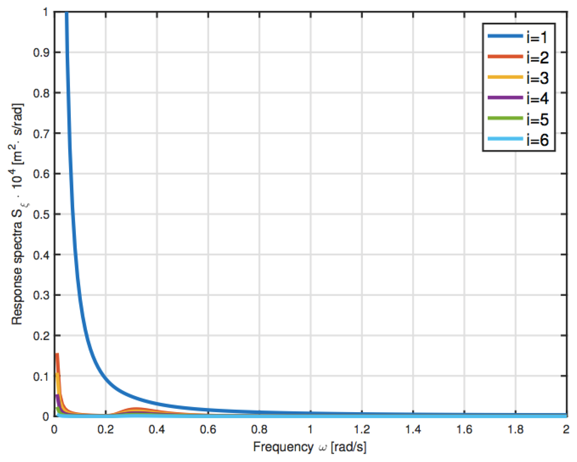
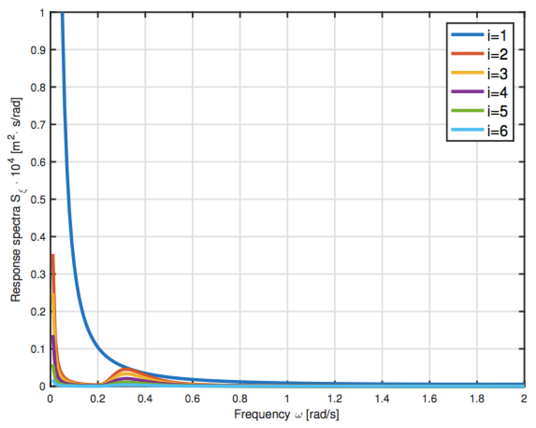
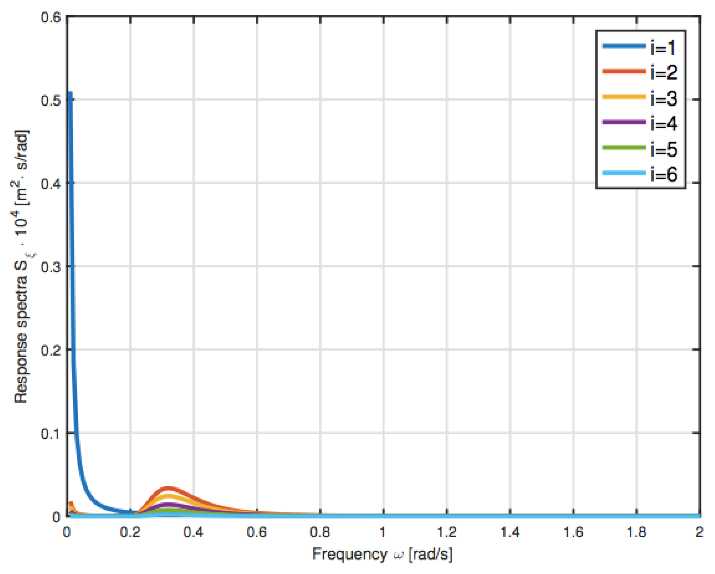
The ninth step is focused on the spectral density in terms of modal coordinates, and it is given by $S(y_k,\omega )={\left|H_k\left(\omega \right)\right|}^{2}S({\overline{q}}_k,\omega )$ with $k=1,2,\dots ,5$. $S({\overline{q}}_k,\omega )$ is the spectral density function of the generalized force component in modal coordinates, and $|H_k\left(\omega \right)|={[{({\omega }_k^2-{\omega }^2)}^2+{(2{\zeta }_K{\omega }_k\omega )}^2]}^{-1/2}$ is the modulus of the harmonic response function for the kth mode. Once the spectral density in terms of modal coordinates $S(y_k,\omega )$ has been determined, is possible to define the spectral density in terms of physical coordinates $S({\xi }_k,\omega )={\sum }_{n=1}^N{x}_{kn}^{2}S(y_k,\omega )$ applying the inverse of the modal analysis, as shown in [30] (Figure 7).

The last step includes the stochastic approach design using the $3\sigma$ approach. By computing the area covered by the response displacement spectra, the variance of such displacement can be carried out ${\sigma }^2\left({\xi }_k\right)$. The extreme limits of ${\xi }_k$ are $\pm 3\sigma \left({\xi }_k\right)$ with $k=1,2,\dots ,5$. If the static stresses and deflection of the members are within these extreme limit values, then the structure is assumed safe. Assuming a Gaussian process, there is only a 0.026% chance that each response exceeds the $\pm 3\sigma \left({\xi }_k\right)$ limits.

The extreme displacement limit values in m are:

$$\begin{array}{c}\hfill 3\sigma \left({\xi }_1\right)=0.3577,3\sigma \left({\xi }_1\right)=0.3158,3\sigma \left({\xi }_1\right)=0.2491,3\sigma \left({\xi }_1\right)=0.1763,3\sigma \left({\xi }_1\right)=0.1014\end{array}$$

(14)

After comparing these results with the maximum peak displacements (Figure 4), the reader will easily state that the structure can be said to be safe.

4. Jacket Supporting the Wind Turbine

The aim of the present paper is to find a useful tool able to model the behavior accurately of a new offshore structure that supports the wind turbine subjected to environmental actions. The structure under investigation presents the same jacket structure with a long pile foundation placed in the same position with the same characteristics. All analysis steps necessary for the simplified design for the new offshore structure have been introduced in the previous section. The introduced 10-step modeling approach will be considered also in the following.

The wind tower is made of steel with a length of 80 m. The nacelle mass is 240 tons. The rotor mass is 110 tons. The turbine diameter is 126 m (Figure 8). The wind tower has a truncated cone shape; at the bottom, the diameter is 4 m and the thickness is 0.18 m; at the top, the diameter is 3.5 m and the thickness is 0.10 m. At half tower height, the diameter is 3.75 m and the thickness is 0.14 m. The hub is at z = +90 m. The wind tower produces a rated power of 5 MW. It is attached to the substructure through a concrete (density 1600 kg/m${}^3$) transition piece with $9.6\times 9.6\times 4$ m${}^3$ of volume. The whole structure will be treated as a discrete system with 5 + 1 lumped masses.

The lumped masses of the jacket are calculated using the same procedure illustrated above. It follows that the mass matrix M of the 6DOF model in kg is:

$$\begin{array}{c}\hfill \mathit{M}=\left[\begin{array}{cccccc}\mathrm{937,000}& 0& 0& 0& 0& 0\\ 0& \mathrm{1,587,300}& 0& 0& 0& 0\\ 0& 0& \mathrm{122,400}& 0& 0& 0\\ 0& 0& 0& \mathrm{147,100}& 0& 0\\ 0& 0& 0& 0& \mathrm{242,300}& 0\\ 0& 0& 0& 0& 0& \mathrm{206,700}\end{array}\right]\end{array}$$

(15)

The stiffness matrix K has been determined along the x direction using the proper definition. Thus, matrix K in N/m is:

$$\begin{array}{c}\hfill \mathit{K}=\left[\begin{array}{cccccc}0.121& -0.121& 0& 0& 0& 0\\ -0.121& 0.6689& -0.6568& 0& 0& 0\\ 0& -0.6568& 1.1290& -0.4722& 0& 0\\ 0& 0& -0.4722& 1.0345& -0.5622& 0\\ 0& 0& 0& -0.5622& 1.1307& -0.5685\\ 0& 0& 0& 0& -0.5685& 1.2073\end{array}\right]·{10}^9\end{array}$$

(16)

The same sea state of the previous section has been considered.

The free undamped motions of the present structure can be determined solving the corresponding eigenvalue problem. The six undamped natural frequencies computed using MATLAB and the FE model are listed in

Table 2. Undamped natural frequencies computed using MATLAB and the FE model.

	MATLAB	FE	Ratio
${\omega }_1$	3.38	3.39	≈1
${\omega }_2$	8.53	8.54	≈1
${\omega }_3$	36.02	36.00	≈1
${\omega }_4$	71.90	71.88	≈1
${\omega }_5$	90.62	90.60	≈1
${\omega }_6$	111.50	111.53	≈1

in rad/s.

${\omega }_1=3.3879$, ${\omega }_2=8.5393$, ${\omega }_3=36.0211$, ${\omega }_4=71.8985$, ${\omega }_5=90.6182$, ${\omega }_6=111.5014$.

The modal shape matrix X of the 6DOF model is defined as the assembly of the normalized modal vectors ${\mathit{x}}_{\mathit{n}}$ as:

$$\begin{array}{c}\hfill \mathit{X}=[{\mathit{x}}_{\mathbf{1}},{\mathit{x}}_{\mathbf{2}},\dots ,{\mathit{x}}_{\mathbf{6}}]=\left[\begin{array}{cccccc}1.0& -0.2& -0.0& 0.0& -0.0& -0.0\\ 0.1& 0.7& 0.2& -0.1& 0.1& 0.1\\ 0.1& 0.6& -0.5& 1.3& -1.3& -2.1\\ 0.1& 0.5& -1.2& 1.5& -0.4& 1.6\\ 0.0& 0.3& -1.5& -0.3& 1.2& -6.0\\ 0.0& 0.1& -0.9& -1.4& -1.4& 0.2\end{array}\right]·{10}^{-3}\end{array}$$

(17)

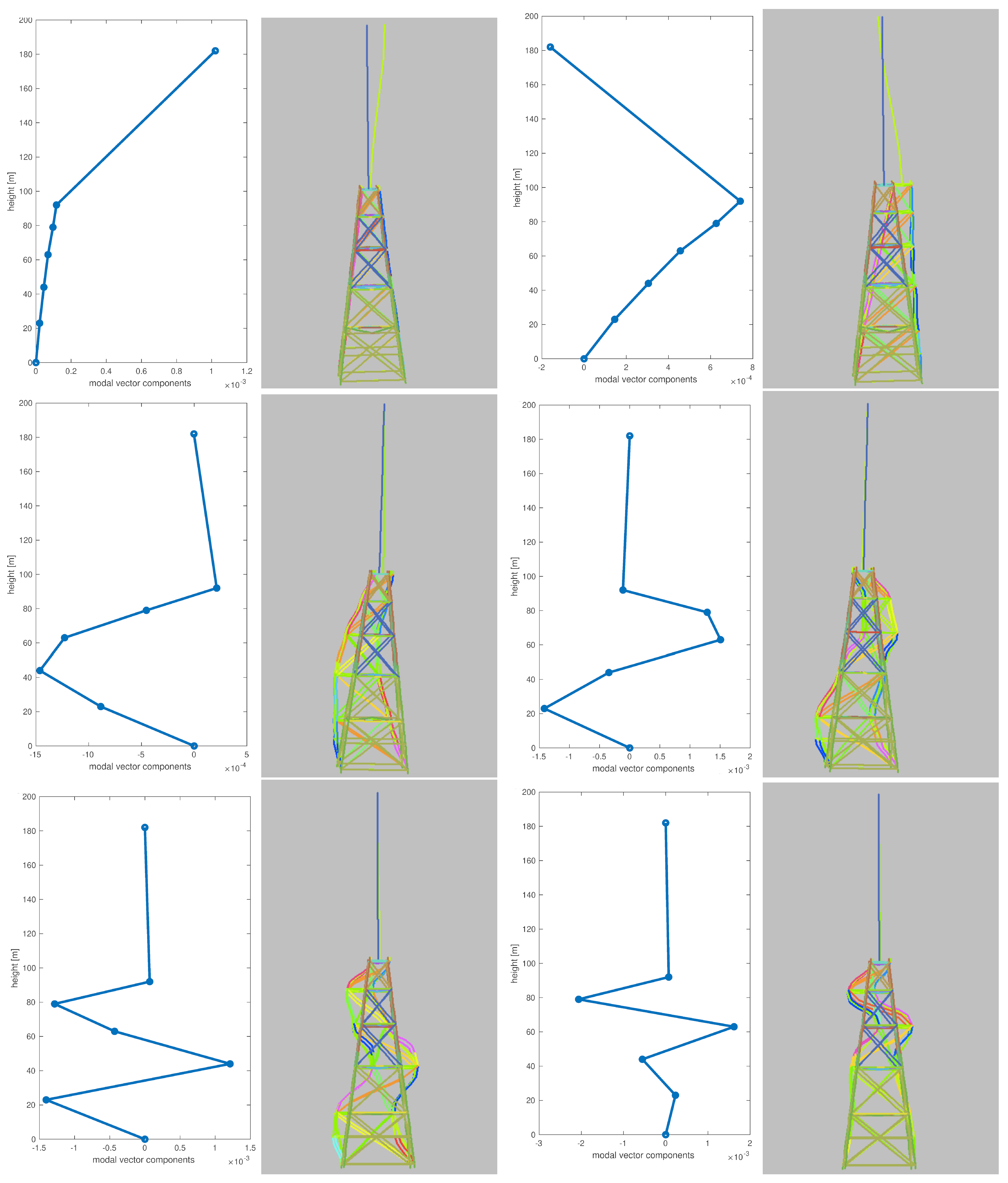
and its vibrational modes of shape are compared to the ones obtained by FE analysis in Figure 9.

As follows, all the frequencies computed via FE analysis in rad/s are: ${\omega }_1=2.74$, ${\omega }_2=7.16$, ${\omega }_3=26.13$, ${\omega }_4=50$, ${\omega }_5=63.81$, and ${\omega }_6=80.39$. The modes of shape obtained by MATLAB calculation and the ones obtained by Strand7 are quite similar, as well as the corresponding natural undamped frequencies. The correlation between the two approaches shows the quality of the model.

As done for the previous case, damped frequencies of the 6DOF model in rad/s are computed as: ${\omega }_{d1}=3.3836$, ${\omega }_{d2}=8.5286$, ${\omega }_{d3}=35.2135$, ${\omega }_{d4}=67.8688$, ${\omega }_{d5}=82.9486$, ${\omega }_{d6}=97.4530$.

The harmonic wave of the previous case is considered below. Regarding the wind load, the correspondent force is calculated at z = +90 m. The wind force is given by two contributions: one from the wind acting against the swept rotor area and the other from the wind acting against the tower. The force considered at the top node of the model $p_1=3055$ kN will take into account the wind on the swept rotor area and the wind on the half tower. The remaining half part of the wind on the tower will be add to the first wave load. The wind force is given by two contributions: one from the wind acting against the swept rotor area and the other from the wind acting against the tower. The force considered at the top node of the model $p_1$ will take into account the wind on the swept rotor area and the wind on the half tower. The remaining half part of the wind on the tower will be added to the first wave load. The counterpart wind on the tower is calculated by integrating the wind velocity over the tower height, and it is equal to $f_w=\int u\left(z\right)dz=191.58$ N with $u\left(z\right)=1.5{(z/3)}^{1/7}$ and with $0\le z\le 90$ m. The counterpart wind on the rotor is $f_{rot}=0.5\rho u_{rot}A=3054.9$ kN, where the wind velocity at the rotor hub is $u_{rot}=20$ m/s. It follows that the wind load applied at the top of the wind turbine is $p_1=f_w/2+f_{rot}=3055$ kN.

The pile foundation check is carried out as previously described with reference to Figure 10. For this new configuration, the maximum compression value in the piles given in B-1 is equal to $FB1=$ −21,131 kN. The same pile in the 5DOF configuration withstood a compression equal to $FB1=-8316$ kN. In the new configuration, the pile B-1 carries more than two and half-times the stress carried in the previous one. Supposing that the compression threshold pile limit is $Fmax=$ −18,000 kN, it is quite clear that the new load produced by the 6DOF configuration is no longer bearable for the pile B-1.

The generic long steel pile foundation in this structure presents the following characteristics: diameter of 2.13 m, wall thickness of 50 mm, pile length of 96 m, of which 75 m are embedded. The corresponding axial pile capacity is $Q_r=$ 28,800 kN. In order to take into account the differences between the structure with the cantilever model, a safety factor equal to ${\gamma }_r=1.60$ has been chosen. It follows that the maximum bearing load for the pile is $F_{max}=Q_r/{\gamma }_r=$ 18,000 kN.

Performing the static analysis with Strand7 of the 6DOF model, the maximum displacement for each node is: ${\xi }_1=1.3893$, ${\xi }_2=0.1012$, ${\xi }_3=0.712$, ${\xi }_4=0.434$, ${\xi }_5=0.0244$, ${\xi }_6=0.0103$.

These values will be compared with the $3\sigma \left({\xi }_k\right)$ approach below.

Although the jacket substructure has the same configuration as the 5DOF model, the wave transfer functions are not identical, but similar to the previous case. This is due to the mode shape matrix X of the 6DOF model. It follows that the equations are the same as the 5DOF configuration, but the functions of the five wave transfer functions are slightly different.

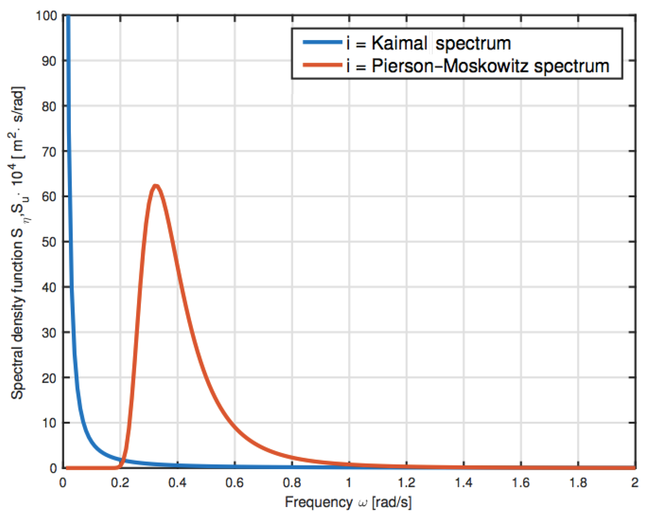
In order to define the spectral density function of the generalized force component, it is requested to define first the wave and wind spectra. For the wind analysis, the Kaimal spectrum is used. The parameters chosen for the Kaimal spectrum are:

$$S_u\left(\omega \right)={\sigma }_U^2\frac{6.868\frac{L_u}{U_{mean}}}{{(1+10.32\frac{\omega L_u}{U_{mean}})}^{5/3}}$$

(18)

where the mean wind velocity $U_{mean}=6$ m/s, the variance of the wind speed ${\sigma }_U^2={\lambda }_w^2·(\Gamma (1+\frac{2}{k_w}-{(\Gamma (1+\frac{1}{k_w}))}^2=12.81$ (m/s)${}^2$ with ${\lambda }_w=6.7$ and $k_w=1.72$ Weibull parameters of probability density of gamma function $\Gamma$, roughness parameter $z_0=0.001$, the integral length scale $L_u=300{(\frac{e{l}_1}{300})}^{0.46+0.074log\left(z_0\right)}=321$ m, and the air density ${\rho }_{air}=1.225$ kg/m${}^3$ (Figure 11).

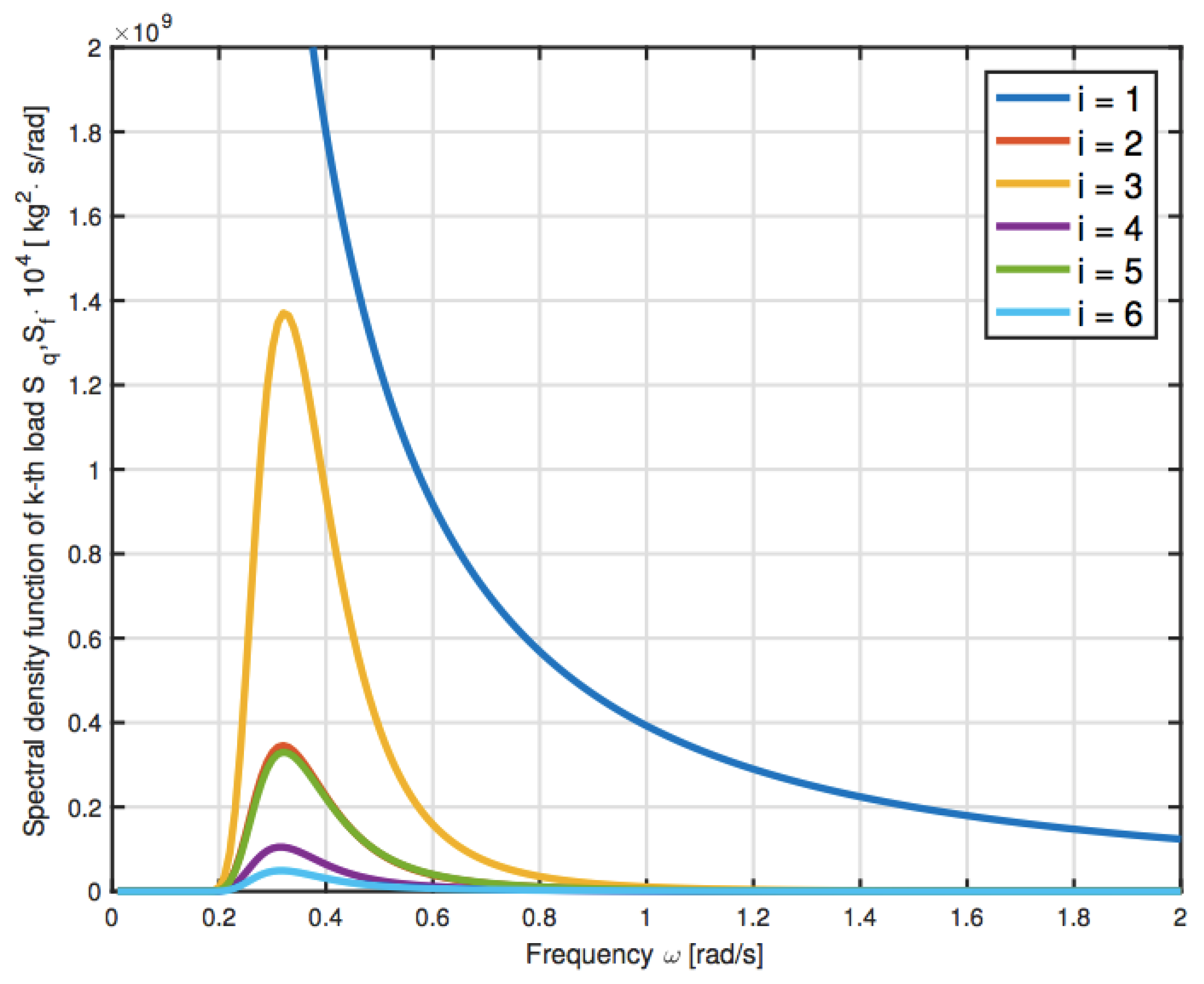
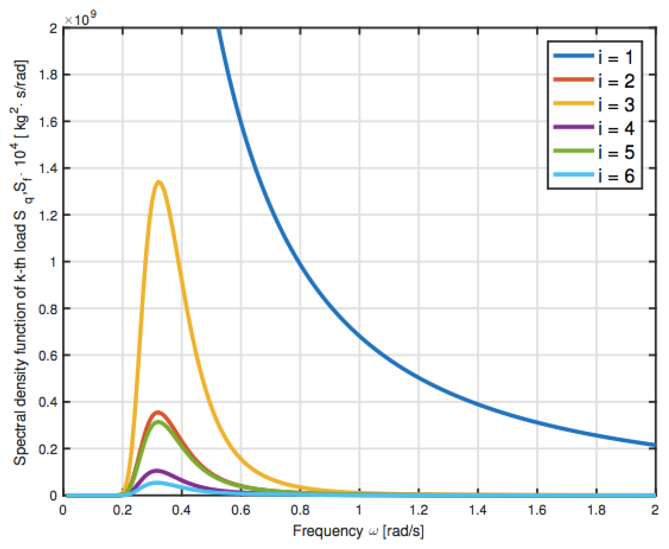
Wave modeling is carried out using the Pierson–Moskowitz spectrum. Multiplying the wind transfer function of the load $H_{uf}=C_{T}A{\rho }_{air}{U}_{mean}$ in the modal coordinates with the thrust coefficient $C_T=0.8$ by the Kaimal spectrum $S_u$ for the wind and the wave transfer functions $|{\mathit{x}}_{\mathit{k}}^{\mathit{T}}{\mathit{G}(p,\omega )|}^2$ by the Pierson–Moskowitz $S_{\eta }$, the spectral density function of the wind force in modal coordinates $S_f=H_{uf}^2·S_u$ and the spectral density of the generalized wave force in modal coordinates $S_{qi}$, respectively, are achieved (Figure 12).

The spectral density of the wind load in modal coordinates $i=1$ has values much higher than the wave loads; in particular, it tends to infinity when $\omega$ tends to zero. For the sake of simplicity, the spectral density function of the wind force in modal coordinates will be limited. The wind transfer function of the load $H_{uf}$ in modal coordinates, which converts the wind speed spectrum to the wind load spectrum, is based on the assumption that $u\left(t\right)$ has the same value over the area, which in general is not true.

Once the spectral density function of the wind load and generalized wave component are defined in modal coordinates $S_f$ and $S_{qi}$, the wind transfer function from the spectral density of wind force into spectral density in modal coordinates is carried out as:

$$|H_{wind}{\left(\omega \right)|}^2=\frac{1}{m_i·4\pi {\omega }_i^4}\frac{1}{{\{1-{(\frac{\omega }{{\omega }_i})}^2\}}^2+4{\zeta }_i^2{(\frac{\omega }{{\omega }_i})}^2}$$

(19)

and the wave transfer functions from spectral density of the generalized wave force component into spectral density in modal coordinates $|H_k{\left(\omega \right)|}^2$. The spectral density function in terms of modal coordinates $S(y_k,\omega )$ is given by multiplying the spectral density function of the load in modal coordinates with the correspondent transfer function in modal coordinates. Let $J_1$ be the joint acceptance of the mode, which accounts for the correlation of wind loading along the rotor, considering the mode shape.

$$J_1=\frac{1}{{\mathit{X}}^4}{\left|H_{wind}\left(\omega \right)\right|}^2$$

(20)

Once the spectral density in terms of modal coordinates $S\left(y_{,}\omega \right)$ has been determined, it is possible to define the spectral density in terms of physical coordinates $S({\xi }_k,\omega )$ (Figure 13).

The last 10-step methodology phase defines the variance of the structural displacements in physical coordinates ${\sigma }^2\left({\xi }_k\right)$. The extreme limits of ${\xi }_k$ are $\pm 3\sigma \left({\xi }_k\right)$ with $k=1,2,\dots ,6$. If the static stresses and deflection of the members are within these extreme limit values, then the structure is assumed safe. Considering a Gaussian process, there is only a 0.026% chance that each response exceeds the $\pm 3\sigma \left({\xi }_k\right)$ limits. The extreme displacement values of the 6DOF configuration in m are: $3\sigma \left({\xi }_1\right)=1.3822$, $3\sigma \left({\xi }_2\right)=0.3471$, $3\sigma \left({\xi }_3\right)=0.2917$, $3\sigma \left({\xi }_4\right)=0.2154$, $3\sigma \left({\xi }_5\right)=0.1505$, $3\sigma \left({\xi }_6\right)=0.0748$. After comparing these results with the ones given above, it can be stated that the structure cannot be safe for the first node at the top of the wind tower, in particular ${\xi }_1=1.40$ m, whereas the limit is $3\sigma \left({\xi }_1\right)=1.38$ m. The 6DOF model built from the adaptation and extension of the 5DOF model has to be modified in order to find the safety condition. In order to do that, hereafter, different retrofitting examples will be presented.

5. Improved Retrofitting Models

Retrofitting refers to the addition of new technology or features to older systems, extending the service life. In this case, different retrofitting typologies are illustrated. The retrofitting models proposed in this section are analyzed following the same methodology previously shown. The approach is suitable for tender design and early design steps of jacket structures. The aim is to identify a useful tool that is able to represent the behavior of the new offshore structure subjected to environmental actions. The system under investigation presents the same jacket and a big wind tower installed on top of it. The whole system will be analyzed with MATLAB calculation and supported by Strand7 software. The aim is to find the right intervention that will ensure the modified offshore structure without causing stability trouble for the system. This research proposes three main retrofitting activities that can be adopted for the offshore wind turbine. They are: crown pile, mooring lines, and 2-MW wind turbine.

5.1. Crown Pile Configuration

The crown pile solution represents the same configuration of the 6DOF model except for the piles at the base of the jacket. In addition to the four corner piles, here there are an extra four piles placed at the midspan of each side at $z=-d$ connected each to the other piles with a rectangular ring (Figure 14). Regarding Figure 14 and all the following configurations, $z=-d$ represents the sea bottom level when the vertical axis z is zero at the Still Water Line (SWL) pointing upward. The reference system shown in Figure 14 of the FE model considers the reference system at the sea bottom, so $z=0$. However, all the present MATLAB models consider the z axis pointing upward with the sea bottom at $z=-d$.

The difference from the previous model is in the definition of the mass matrix M, where the mass $m_6=$ 19,202 kg. The six undamped natural structural frequencies for free vibration in rad/s are: ${\omega }_1=3.3879$, ${\omega }_2=8.5391$, ${\omega }_3=35.7613$, ${\omega }_4=70.5186$, ${\omega }_5=89.1430$, ${\omega }_6=111.4539$. For the nth frequency ${\omega }_n$ exists a modal vector ${\xi }^n$, which can be computed solving the linear eigenvalue problem (see [30] p. 226).

The crown pile mode shapes are represented in Figure 15.

The damped frequencies of the 6DOF model in rad/s are: ${\omega }_{d1}=3.3837$, ${\omega }_{d2}=8.5284$, ${\omega }_{d3}=34.9825$, ${\omega }_{d4}=66.6939$, ${\omega }_{d5}=81.8239$, ${\omega }_{d6}=97.4230$.

Wave and wind loads do not change with respect to the previous 6DOF case.

The pile foundation check leads to a maximum compression in the pile B-1 equal to $F_{B1}=$ −17,178 kN lower than the pile compression limit $F_{max}=$ −18,000 kN. The reader can easily state that this first configuration helps the wind turbine in terms of stability. The maximum node displacements of the crown pile model in m are: ${\xi }_1=1.3893$, ${\xi }_2=0.1011$, ${\xi }_3=0.711$, ${\xi }_4=0.433$, ${\xi }_5=0.0243$, ${\xi }_6=0.0101$. These values will be compared with the results obtained with the $3\sigma \left({\xi }_k\right)$ approach to ensure structural safety.

The five wave transfer function are rather similar to the ones obtained for the 6DOF.

Multiplying the wind transfer function of the load $H_{uf}$ in modal coordinates by the Kaimal spectrum $S_u$ for the wind and the wave transfer functions $|{\mathit{x}}_{\mathit{k}}^{\mathit{T}}{\mathit{G}(p,\omega )|}^2$ by the Pierson–Moskowitz $S_{\eta }$, the spectral density function of the wind force in modal coordinates $S_f$ and the spectral density of the generalized wave force in modal coordinates $S_{qi}$, respectively, are achieved. Such spectral densities are depicted in Figure 16.

The response spectra (Figure 17) for the displacements in physical coordinates of the offshore wind turbine crown pile configuration have been determined.

The area beneath these spectral density functions represents the variance of the generic displacement in physical coordinates ${\sigma }^2\left({\xi }_k\right)$. The extreme limits of ${\xi }_k$ are $\pm 3\sigma \left({\xi }_k\right)$ with $k=1,2,\dots ,6$. If the static stresses and deflection of the members are within these extreme limit values, then the structure is assumed safe. Considering a Gaussian process, there is only a 0.026% chance that each response exceeds the $\pm 3\sigma \left({\xi }_k\right)$ limits.

The extreme displacement values of the crown pile configuration in m are: $3\sigma \left({\xi }_1\right)=1.3821$, $3\sigma \left({\xi }_2\right)=0.3470$, $3\sigma \left({\xi }_3\right)=0.2916$, $3\sigma \left({\xi }_4\right)=0.2152$, $3\sigma \left({\xi }_5\right)=0.1503$, $3\sigma \left({\xi }_6\right)=0.0751$.

Comparing these results with the ones given by Figure 15, the reader will easily state that the structure cannot be safe for the first node at the top of the wind tower, in particular ${\xi }_1=1.3893$ m and $3\sigma \left({\xi }_1\right)=1.3821$. The crown pile configuration has obtained higher values of safety expressed by the $3\sigma \left(\xi \right)$ approach results, but this is not enough yet for the global stability.

5.2. Mooring Line Configuration

The mooring line configuration presents the same configuration of the 6DOF model, which in addition has a mooring line system that links the midspan second horizontal plane point of the jacket to the seabed, limiting the movement (Figure 18). The mooring line has been modeled as a steel truss element subjected to tension action given by the environmental loads. It has a diameter cross-section of 0.1 m and a length of 98 m, and it creates an angle of ${60}^{\circ }$ with the seabed. For this proposal, only the x direction will be considered, but for real cases, it could be extended and applied for each direction.

The mooring line masses are calculated following the same approach shown previously. Here, the mooring pile configuration mass matrix M in kg:

$$\begin{array}{c}\hfill \mathit{M}=\left[\begin{array}{cccccc}0.9370& 0& 0& 0& 0& 0\\ 0& 1.5873& 0& 0& 0& 0\\ 0& 0& 0.1224& 0& 0& 0\\ 0& 0& 0& 0.1471& 0& 0\\ 0& 0& 0& 0& 0.2423& 0\\ 0& 0& 0& 0& 0& 0.2067\end{array}\right]·{10}^6\end{array}$$

(21)

The stiffness matrix K has been determined over the x direction. Once having applied the definition of stiffness to all the system, it is possible to define the matrix K in N/m as:

$$\begin{array}{c}\hfill \mathit{K}=\left[\begin{array}{cccccc}0.121& -0.121& 0& 0& 0& 0\\ -0.121& 0.6689& -0.6568& 0& 0& 0\\ 0& -0.6568& 1.1342& -0.4722& 0& 0\\ 0& 0& -0.4722& 0.9560& -0.4838& 0\\ 0& 0& 0& -0.4838& 1.0523& -0.5685\\ 0& 0& 0& 0& -0.5685& 1.0390\end{array}\right]·{10}^9\end{array}$$

(22)

The sea state is unchanged with respect to the previous cases.

The six undamped natural structural frequencies for free vibration in rad/s are: ${\omega }_1=3.3737$, ${\omega }_2=8.2907$, ${\omega }_3=33.7583$, ${\omega }_4=67.6558$, ${\omega }_5=87.5002$, ${\omega }_6=111.0619$. Natural frequencies of the present case are depicted in Figure 19.

The response of the mooring line configuration to the harmonic waves has been considered using the same hypothesis for the 6DOF model. The wave loads and the wind load present the same values for the 6DOF system.

A foundation check is performed for both the piles and the mooring line anchoring. The tension in the mooring line from Strand7 calculation is $F_{ml}=427.5$ kN. The calculation of the stress applied on the pile B-1 considers all the environmental loads $p_i$ with the horizontal and vertical component of $F_{ml}$ that are applied to the structure. The compression in the pile B-1 is equal to $F_{B1}=$ −20,959 kN, which is still too high for the compression pile limit capacity.

The damped frequencies of the 6DOF model in rad/s are: ${\omega }_{d1}=3.3695$, ${\omega }_{d2}=8.2803$, ${\omega }_{d3}=33.0309$, ${\omega }_{d4}=64.0793$, ${\omega }_{d5}=80.2370$, ${\omega }_{d6}=95.8081$.

The maximum nodal displacements of the mooring model in m are: ${\xi }_1=1.3854$, ${\xi }_2=0.0983$, ${\xi }_3=0.0685$, ${\xi }_4=0.0416$, ${\xi }_5=0.0235$, ${\xi }_6=0.0099$. These values will be then compared with the results obtained with the $3\sigma \left({\xi }_k\right)$ for checking structural safety.

The five wave transfer functions are similar to the ones obtained for the previous case.

Multiplying the wind transfer function of the load $H_{uf}$ in modal coordinates by the Kaimal spectrum $S_u$ for the wind and the wave transfer functions $|{\mathit{x}}_{\mathit{k}}^{\mathit{T}}{\mathit{G}(p,\omega )|}^2$ by the Pierson–Moskowitz $S_{\eta }$, the spectral density function of the wind force in modal coordinates $S_f$ and the spectral density of the generalized wave force in modal coordinates $S_{qi}$, respectively, are achieved. These spectra are illustrated by Figure 20.

The response spectra (Figure 21) for the displacements in physical coordinates of the offshore wind turbine crown pile configuration have been determined.

The area beneath these spectral density functions represents the variance of the generic displacement in physical coordinates ${\sigma }^2\left({\xi }_k\right)$. The extreme limits of ${\xi }_k$ are $\pm 3\sigma \left({\xi }_k\right)$ with $k=1,2,\dots ,6$. If the static stresses and deflection of the members are within these extreme limit values, then the structure is assumed safe. Considering a Gaussian process, there is only a 0.026% chance that each response exceeds the $\pm 3\sigma \left({\xi }_k\right)$ limits. The extreme displacement values of the crown pile configuration in m are: $3\sigma \left({\xi }_1\right)=1.3965$, $3\sigma \left({\xi }_2\right)=0.3768$, $3\sigma \left({\xi }_3\right)=0.3204$, $3\sigma \left({\xi }_4\right)=0.2459$, $3\sigma \left({\xi }_5\right)=0.1724$, $3\sigma \left({\xi }_6\right)=0.0995$.

Comparing these results with the ones previously given, the reader will easily state that the structure cannot be safe for the first node at the top of the wind tower, in particular ${\xi }_1=1.3854$ m and $3\sigma \left({\xi }_1\right)=1.3965$. The mooring configuration has obtained higher values of safety expressed by the $3\sigma \left(\xi \right)$ approach results, but it is not enough yet for the global stability.

5.3. The 2-MW Wind Turbine Configuration

The modeling of the 2-MW configuration is characterized by the same jacket sub-structure, but with a smaller wind tower. Tower length is 60 m. The nacelle mass is 57 tons. The rotor mass is 23 tons. The diameter is 66 m. The wind tower has a truncated cone shape. At the bottom, the diameter is 4 m and the thickness is 0.18 m. At the top, the diameter is 3.5 m and the thickness is 0.10 m. At half the tower height, the diameter is 3.75 m and the thickness is 0.14 m. The hub is at z = +70 m. The wind tower produces a rated power of 2 MW. As for the 6DOF model, it is attached to the sub-structure through the same concrete transition piece. The sketch of the 2-MW offshore wind turbine configuration is given in Figure 22.

All the masses have been calculated considering the specific weight of the steel 7850 kg/m${}^3$ multiplied by the generic cross-section and multiplied by the length of the tubular member. It follows that the mass matrix M of the 6DOF model in kg is:

$$\begin{array}{c}\hfill \mathit{M}=\left[\begin{array}{cccccc}0.5203& 0& 0& 0& 0& 0\\ 0& 1.4834& 0& 0& 0& 0\\ 0& 0& 0.1224& 0& 0& 0\\ 0& 0& 0& 0.1471& 0& 0\\ 0& 0& 0& 0& 0.2423& 0\\ 0& 0& 0& 0& 0& 0.2067\end{array}\right]·{10}^6\end{array}$$

(23)

The stiffness matrix K has been determined over the x direction. Once having applied the definition of stiffness to all the system, it is possible to define the matrix K in N/m as:

$$\begin{array}{c}\hfill \mathit{K}=\left[\begin{array}{cccccc}0.121& -0.121& 0& 0& 0& 0\\ -0.121& 0.6689& -0.6568& 0& 0& 0\\ 0& -0.6568& 1.1290& -0.4722& 0& 0\\ 0& 0& -0.4722& 1.0345& -0.5622& 0\\ 0& 0& 0& -0.5622& 1.1307& -0.5685\\ 0& 0& 0& 0& -0.5685& 1.2073\end{array}\right]·{10}^9\end{array}$$

(24)

The sea state remains unchanged with respect to the other configurations.

The six undamped natural structural frequencies for free vibration in rad/s are: ${\omega }_1=4.5039$, ${\omega }_2=8.8834$, ${\omega }_3=36.1127$, ${\omega }_4=71.9487$, ${\omega }_5=90.6417$, ${\omega }_6=111.5328$. They are also graphically represented in Figure 23.

The damped frequencies of the 6DOF model in rad/s are: ${\omega }_{d1}=4.4983$, ${\omega }_{d2}=8.8723$, ${\omega }_{d3}=35.5149$, ${\omega }_{d4}=68.8136$, ${\omega }_{d5}=84.6690$, ${\omega }_{d6}=100.6118$.

The response of the harmonic wave has been considered the same as the 6DOF model. The wind load due to the different wind towers will be lower in particular if it is applied at z = +70 m and is equal to $P_w=838$ kN.

The compression in the pile B1 is equal to $F_{B1}=$ −13,288 kN, lower than the compression limit value of the pile.

The maximum node displacements of the mooring model in m are: ${\xi }_1=0.2989$, ${\xi }_2=0.0504$, ${\xi }_3=0.0413$, ${\xi }_4=0.0302$, ${\xi }_5=\mathrm{0.0.0194}$, ${\xi }_6=0.0099$. These values will be then compared with the results obtained with the $3\sigma \left({\xi }_k\right)$ approach that will define the structural safety.

The five wave transfer functions are similar to the ones obtained for the previous cases.

Multiplying the wind transfer function of the load $H_{uf}$ in modal coordinates by the Kaimal spectrum $S_u$ for the wind and the wave transfer functions $|{\mathit{x}}_{\mathit{k}}^{\mathit{T}}{\mathit{G}(p,\omega )|}^2$ by the Pierson–Moskowitz $S_{\eta }$, the spectral density function of the wind force in modal coordinates $S_f$ and the spectral density of the generalized wave force in modal coordinates $S_{qi}$, respectively, are achieved (Figure 24).

For the spectral density of the wind load in modal coordinates, the same consideration is made for the 6DOF case.

As done for the previous model, the response spectra for the displacements in physical coordinates of the offshore wind turbine crown pile configuration have been determined and are shown in Figure 25.

The area beneath these spectral density functions represents the variance of the generic displacement in physical coordinates ${\sigma }^2\left({\xi }_k\right)$. The extreme limits of ${\xi }_k$ are $\pm 3\sigma \left({\xi }_k\right)$ with $k=1,2,\dots ,6$. If the static stresses and deflection of the members are within these extreme limit values, then the structure is assumed safe. Considering a Gaussian process, there is only a 0.026% chance that each response exceeds the $\pm 3\sigma \left({\xi }_k\right)$ limits.

The extreme displacement values of the 2-MW wind turbine configuration in m are: $3\sigma \left({\xi }_1\right)=0.4208$, $3\sigma \left({\xi }_2\right)=0.1847$, $3\sigma \left({\xi }_3\right)=0.1572$, $3\sigma \left({\xi }_4\right)=0.1234$, $3\sigma \left({\xi }_5\right)=0.0950$, $3\sigma \left({\xi }_6\right)=0.0503$.

Comparing these results with the ones given above, the reader will easily state that the structure cannot be safe for the first node at the top of the wind tower, in particular ${\xi }_1=0.2989$ m and $3\sigma \left({\xi }_1\right)=0.4208$. The 2-MW configuration has obtained lower values of safety expressed by the $3\sigma \left(\xi \right)$ approach results and together with the pile check analysis completes the global stability of the 2-MW retrofitted configuration.

6. Conclusions

Due to the long service lifetime of offshore systems, the analysis of the performance of the substructure is a complex task that involves many steps including load analysis, dynamic analysis, evaluation of the fatigue life, as well as long-term deformations.

This work presents a simplified methodology for the analysis of the ultimate and dynamic loads with a check on the most stressed pile of the different offshore retrofitted systems. The analysis was carried out such that the data required about the oil and gas platform, wind turbines, and the site are available in the early design phases. Thus, the methodology appears to obtain a conservative estimation. It is obvious that the present study is not free from limitations, but it can be improved in further investigations.

The first limitation is due to the simplified modeling made of discrete masses, one for each jacket level. Nevertheless, high correlations have been shown with the example proposed by the references.

The present work proposes five retrofitted solutions: four related to the substructure operations and one regarding the wind turbine. They are respectively the crown pile configuration, long pile, mooring line, stirrups, and the 2-MW wind turbine configuration. The safety concept of the retrofitted models is expressed in terms of pile check analysis and the $3\sigma$ approach.

Nevertheless, the final values obtained by the different configuration typologies are slightly higher or lower than the threshold limit, and the check is slightly fulfilled or not; here, the goal is just to show a simple method to investigate an offshore structure. The present research can be considered as the starting point for a reliability analysis regarding decommissioned jacket platforms for wind energy generations in an offshore environment.

References

- Muskulus, M.; Schafhirt, S. Design Optimization of Wind Turbine Support Structures—A Review. J. Ocean Wind Energy 2014, 1, 12–22. [Google Scholar]
- International Energy Agency. Offshore Energy Outlook; International Energy Agency: Paris, France, 2018. [Google Scholar]
- Global Wind Energy Council (GWEC). Global Wind Report 2015; Technical Report; Global Wind Energy Council: Brussels, Belgium, 2016. [Google Scholar]
- Huang, W.; Liu, J.; Zhao, Z. The state of the art of study on offshore wind turbine structures and its development. Ocean Eng. 2009, 2. Available online: http://en.cnki.com.cn/Article_en/CJFDTOTAL-HYGC200902021.htm (accessed on 10 February 2018).
- Ho, A.; Mbistrova, A. The European Offshore Wind Industry: Key Trends and Statistics 2016; Technical Report; WindEurope: Brussels, Belgium, 2017. [Google Scholar]
- ORE Catapult. Cost Reduction Monitoring Framework 2016: Summary Report to the Offshore Wind Programme Board; Technical Report; Offshore Renewable Energy Catapult: Glasgow, UK, 2017. [Google Scholar]
- Mone, C.; Stehly, T.; Maples, B.; Settle, E. 2014 Cost of Wind Energy Review; National Renewable Energy Laboratory: Oak Ridge, TN, USA, 2015.
- Musial, W.D.; Sheppard, R.E.; Dolan, D.; Naughton, B. Development of Offshore Wind Recommended Practice for U.S. Waters. In Proceedings of the Offshore Technology Conference Houston, Texas, TX, USA, 6–9 May 2013. [Google Scholar]
- Veldkamp, D. A probabilistic evaluation of wind turbine fatigue design rules. Wind Energy 2008, 11, 655–672. [Google Scholar] [CrossRef] [Green Version]
- DNV GL. DNVGL-ST-0437: Loads and Site Conditions for Wind Turbines. Available online: https://rules.dnvgl.com/docs/pdf/DNVGL/ST/2016-11/DNVGL-ST-0437.pdf (accessed on 10 February 2018).
- Negro, V.; Lopez-Gutierrez, J.-S.; Esteban, M.D.; Matutano, C. Uncertainties in the design of support structures and foundations for offshore wind turbines. Renew. Energy 2014, 63, 125–132. [Google Scholar] [CrossRef] [Green Version]
- Seidel, M. Jacket substructures for the REpower 5M wind turbine. In Proceedings of the Conference Proceedings European Offshore Wind, Berlin, Germeny, 4–6 December 2007; Available online: http://www.marc-seidel.de/Papers/Seidel_EOW_2007.pdf (accessed on 10 February 2018).
- Lozano-Minguez, E.; Kolios, A.J.; Brennan, F.P. Multi-criteria assessment of offshore wind turbine support structures. Renew. Energy 2011, 36, 2831–2837. [Google Scholar] [CrossRef] [Green Version]
- Popko, W.; Vorpahl, F.; Zuga, A.; Kohlmeier, M.; Jonkman, J.; Robertson, A.; Larsen, T.J.; Yde, A.; Sætertrø, K.; Okstad, K.M.; et al. Offshore Code Comparison Collaboration Continuation (OC4), Phase I—Results of Coupled Simulations of an Offshore Wind Turbine with Jacket Support Structure. In Proceedings of the Twenty-second International Offshore and Polar Engineering Conference, Rhodes, Greece, 17–22 June 2012. [Google Scholar]
- Saha, N.; Gao, Z.; Moan, T.; Naess, A. Short-term extreme response analysis of a jacket supporting an offshore wind turbine. Wind Energy 2014, 17, 87–104. [Google Scholar] [CrossRef]
- Luo, T.; Tian, D.; Wang, R.; Liao, C. Stochastic Dynamic Response Analysis of a 10 MW Tension Leg Platform Floating Horizontal Axis Wind Turbine. Energies 2018, 11, 3341. [Google Scholar] [CrossRef]
- Sivalingam, K.; Martin, S.; Wala, A.A.S. Numerical Validation of Floating Offshore Wind Turbine Scaled Rotors for Surge Motion. Energies 2018, 11, 2578. [Google Scholar] [CrossRef]
- Ku, C.-Y.; Chien, L.-K. Modeling of Load Bearing Characteristics of Jacket Foundation Piles for Offshore Wind Turbines in Taiwan. Energies 2016, 9, 625. [Google Scholar] [CrossRef]
- Chen, I.-W.; Wong, B.-L.; Lin, Y.-H.; Chau, S.-W.; Huang, H.-H. Design and Analysis of Jacket Substructures for Offshore Wind Turbines. Energies 2016, 9, 264. [Google Scholar] [CrossRef]
- Chew, K.H.; Ng, E.Y.K.; Tai, K. Offshore Wind Turbine Jacket Substructure: A Comparison Study Between Four-Legged and Three-Legged Designs. J. Ocean Wind Energy 2014, 1, 74–81. [Google Scholar]
- Chew, K.H.; Ng, E.Y.K.; Tai, K.; Muskulus, M.; Zwick, D. Structural Optimization and Parametric Study of Offshore Wind Turbine Jacket Substructure. In Proceedings of the Twenty-Third International Offshore and Polar Engineering Conference, Anchorage, AK, USA, 30 June–5 July 2013. [Google Scholar]
- Dubois, J.; Muskulus, M.; Schaumann, P. Advanced Representation of Tubular Joints in Jacket Models for Offshore Wind Turbine Simulation. Energy Procedia 2013, 35, 234–243. [Google Scholar] [CrossRef] [Green Version]
- Kang, J.; Liu, H.; Fu, D. Fatigue Life and Strength Analysis of a Main Shaft-to-Hub Bolted Connection in a Wind Turbine. Energies 2019, 12, 7. [Google Scholar] [CrossRef]
- Liu, F.; Li, H.; Li, W.; Wang, B. Experimental study of improved modal strain energy method for damage localisation in jacket-type offshore wind turbines. Renew. Energy 2014, 72, 174–181. [Google Scholar] [CrossRef]
- Abkar, M. Theoretical Modeling of Vertical-Axis Wind Turbine Wakes. Energies 2019, 12, 10. [Google Scholar] [CrossRef]
- Palmieri, M.; Bozzella, S.; Cascella, G.L.; Bronzini, M.; Torresi, M.; Cupertino, F. Wind Micro-Turbine Networks for Urban Areas: Optimal Design and Power Scalability of Permanent Magnet Generators. Energies 2018, 11, 2759. [Google Scholar] [CrossRef]
- Wicaksono, Y.A.; Prija Tjahjana, D.D.D.; Hadi, S. Influence of omni-directional guide vane on the performance of cross-flow rotor for urban wind energy. AIP Conf. Proc. 2018, 1931, 030040. [Google Scholar] [CrossRef]
- Farhan, M.; Mohammadi, M.R.S.; Correia, J.A.; Rebelo, C. Transition piece design for an onshore hybrid wind turbine with multiaxial fatigue life estimation. Wind Eng. 2018, 42, 286–303. [Google Scholar] [CrossRef]
- Mourao, A.; Correia, J.A.F.O.; Castro, J.M.; Correia, M.; Leziuk, G.; Fantuzzi, N.; De jesus, A.M.P.; Calcada, R.A.B. Fatigue Damage Analysis of Offshore Structures using Hot-Spot stress and Notch Strain Approaches. Mater. Res. Forum 2019, in press. [Google Scholar]
- Wilson, J.F. Dynamics of Offshore Structures; Wiley: Hoboken, NJ, USA, 2002. [Google Scholar]
Figure 1.
Jacket modeled by Strand7 and MATLAB.
Figure 2.
Mode shape comparison between 5DOF and the FE model.
Figure 3.
Pile stress analysis of the 5DOF model.
Figure 4.
Time domain plot of the 5DOF model.
Figure 5.
Wave transfer functions for the 5DOF model.
Figure 6.
Spectral density functions of the generalized force component in modal coordinates for the 5DOF model.
Figure 7.
Response spectra for the displacement in physical coordinates of the fixed-leg platform.
Figure 8.
Wind tower model.
Figure 9.
Vibrational mode comparison between the 6DOF and FE models.
Figure 10.
Pile stress analysis of the 6DOF model.
Figure 11.
Wave and wind spectral density function.
Figure 12.
Spectral density of the generic environmental load in modal coordinates of the 6DOF model.
Figure 13.
Response spectra for the displacement in physical coordinates of the offshore wind turbine plot.
Figure 14.
Crown pile model detail.
Figure 15.
Crown pile vibration modes.
Figure 16.
Crown pile spectral density of the generic environmental load in modal coordinates.
Figure 17.
Response spectra for the displacements in physical coordinates of the offshore wind turbine crown pile configuration.
Figure 18.
Mooring line configuration model detail.
Figure 19.
Mooring line vibrational modes.
Figure 20.
Mooring line spectral density of the generic environmental load in modal coordinates.
Figure 21.
Response spectra for the displacements in physical coordinates of the offshore wind turbine mooring line configuration.
Figure 22.
The 2-MW model detail.
Figure 23.
The 2-MW configuration vibrational modes.
Figure 24.
The 2-MW configuration spectral density of the generic environmental load in modal coordinates.
Figure 25.
Response spectra for the displacements in physical coordinates of the 2-MW offshore wind turbine configuration.