A Numerical Study on the Development of Self-Similarity in a Wind Turbine Wake Using an Improved Pseudo-Spectral Large-Eddy Simulation Solver


1
Key Lab of Structures Dynamic Behavior and Control of the Ministry of Education, Harbin Institute of Technology, Harbin 150090, China
2
Key Lab of Smart Prevention and Mitigation of Civil Engineering Disasters of the Ministry of Industry and Information Technology, Harbin Institute of Technology, Harbin 150090, China
3
Department of Mechanical Engineering and St. Anthony Falls Laboratory, University of Minnesota, Minneapolis, MN 55455, USA
*
Author to whom correspondence should be addressed.
Energies 2019, 12(4), 643; https://doi.org/10.3390/en12040643
Submission received: 9 January 2019
/
Revised: 3 February 2019
/
Accepted: 13 February 2019
/
Published: 17 February 2019
Abstract
:Large-eddy simulation (LES) is performed to investigate self-similarity in a wind turbine wake flow. The turbine is represented using an actuator line model in a pseudo-spectral method-based solver. A new hybrid approach of smoothed pseudo-spectral method and finite-difference method (sPSMFDM) is proposed to alleviate the Gibbs phenomenon caused by the jump of velocity and pressure around the turbine. The LES is validated with the mean velocity and turbulence statistics obtained from wind-tunnel measurement reported in the literature. Through an appropriate choice of characteristic scales of velocity and length, self-similarity is elucidated in the normalized mean velocity and Reynolds stress profiles at various distances. The development of self-similarity is categorized into three stages based on the variation in the characteristic scales and the spanwise distribution of normalized velocity deficit. The mechanisms responsible for the transition of self-similarity stages are analyzed in detail. The findings of the flow physics obtained in this study will be useful for the modeling and fast prediction of wind turbine wake flows.
1. Introduction
Wind power is one of the fastest-growing sources of electricity supply, with advantages in environmental benefits and the abundance in resource [1]. When designing the layout of wind farms, on one hand, it is desirable to have the distance between turbines along the wind direction as short as possible for less land use and lower cost of auxiliary facilities. On the other hand, insufficient distance between turbines leads to less wind energy extraction. The characteristics of the mean velocity in the wake of a turbine is a key factor in determining the lower bound of turbine array spacing.
The mean flow of a turbine wake is influenced by many variables of the ambient flow and the turbine structure. If the turbine rotor is simplified as a static penetrable disc perpendicular to the mean flow, classical boundary-layer theories could provide analytic predictions for the development of the free wake in laminar or turbulent flows [2,3]. The analytic predictions usually start the trial solution from the knowledge in the self-similarity phenomenon, which emphasizes the similarities of the spanwise distribution at various downstream distances. The theoretical solution shows that the inflow velocity, the drag coefficient, and the Reynolds stress are the dominant factors affecting the mean flow in the axisymmetric wake. The drag coefficient of the turbine equals to the thrust coefficient, which can be predicted using the blade element momentum theory (BLMT) [4,5]. Based on the BLMT, the drag coefficient is determined by the blade configuration and tip-speed-ratio. The effect of the ambient turbulence on the wake flow, which accelerates the recovery of velocity [6,7], is reflected in the Reynolds stress term in the boundary-layer equation for the wake flow. The Reynolds stress is often estimated using the mixing-length model [2,8].
In reality, the wake flow of a wind turbine is more complex than the simplified axisymmetric disc wake, owing to the rotation of the blades and the blockage of the nacelle. The rotation of the blades generates helical tip vortices and root vortices. The nacelle reduces the velocity at the center of the rotating plane and generates a secondary wake flow inside the turbine wake. In addition, there exists the phenomenon of wake meandering, which is a large-scale lateral motion of the central low velocity region under the perturbations of ambient turbulent flow. The above various features in the turbine wake may interact with each other. The interaction between tip vortices and disc wake flow has been investigated theoretically [9] and experimentally [10], where the mutual inductance between adjacent spirals is found to be the dominant mechanism for the merging and grouping of tip vortices. For some blade geometries, strong root vortices may form at a relatively large radial distance from the centerline and further interact with the tip vortices [11]. The wake meandering has been studied in laboratory experiments using particle image velocimetry (PIV) [12]. In numerical simulations [13], it is found that the amplitude of wake meandering is proportional to the thrust coefficient and inversely proportional to the frequency of the hub vortices. The mean velocity shear in atmosphere also makes the inflow condition different from that in the classical wake theory. Even so, the high turbulence intensity produced by the large mean velocity shear is found to have stronger effect than the high mean velocity shear itself [7].
Large-eddy simulation (LES) is a powerful and increasingly popular tool in the study of turbine wake flows. The complexity of the wake structure makes it challenging for theoretical and experimental investigation to gather the whole-field data for a wide range of parameters, while setting up cases for phenomena of interests is more flexible in LES. The actuator line method (ALM) and its predecessor actuator disk model (ADM) have been extensively applied in LES to consider the effects of turbine forces on the wake flow with a computational cost lower than the geometry-resolved LES (LES-GR) [14,15,16,17,18,19,20,21,22,23,24,25,26]. While the combination of LES and ALM/ADM (LES-AL and LES-AD) has been widely employed for the estimation of the mean flow and the corresponding wind energy in wind farms [15,17,18,21,23,24,25], less LES studies have been performed to study the mechanisms of the interactions among different flow structures in the turbine wake. Bastankhah and Porté-Agel [27] derived an analytical wake model that assumed a Gaussian distribution for the velocity deficit in the wake while considering the conservations of mass and momentum. They compared the results of the analytical model with wind-tunnel measurements and LES. The analytical model predicted the velocity deficit and power extraction more accurately than previous models that considered a top-hat shape for the velocity deficit [28,29]. Xie and Archer [30] used LES-AL to study the self-similarity of the mean velocity and the added turbulence intensity in a single turbine wake flow. They found that the self-similarity of velocity deficit exists in the horizontal and upper vertical planes, while it breaks down as it gets close to the ground in the lower vertical plane. They proposed to use two different wake widths for horizontal and vertical planes, respectively. Their modified wake model provides better predictions for the mean velocity deficit and turbulence intensity in far wake than previous models [27,28,29]. Kang et al. [19] compared the results of LES-GR and LES-AL, and emphasized the necessity of nacelle modeling in simulations to capture the radial expansion of hub vortex meandering. Foti et al. [31] found that the wavelength of the wake meandering profile becomes larger after the expanding hub vortex intercepts the tip shear layer. These above studies provided quantitative analyses focusing on nacelle model, tip vortices, wake meandering, or specific aspects of the self-similarity. In the present study, the interaction of multiple flow structures in the wake is investigated.
The present work aims to use LES-AL to study the development of self-similarity in the wake of a turbine, including the formation of self-similarity and the influences from dominant flow structures in the wake. The rest of this paper is organized as follows. In Section 2, we provide an overview of the computational framework, which embeds the actuator line model into a spectral solver of LES. A new spectral scheme for calculating derivatives is proposed to alleviate the Gibbs phenomenon observed in the coupling of ALM and spectral solver. In Section 3, we set up a simulation for a miniature turbine in a wind-tunnel test reported in literature. In Section 4.1, we compare the mean velocity, turbulence intensity, and Reynolds stress at two different downstream locations with the wind-tunnel measurements. In Section 4.2, we study the self-similarity of the mean velocity by normalizing the flow field with characteristic scales of velocity and length. In Section 4.3, we present the self-similarity in the Reynolds stress. In Section 4.4, we explain the formation of self-similarity by a budget analysis of the mean momentum equation. In Section 4.5, we analyze the influences of tip vortices and wake meandering, which are assumed to cause the change in the growth rate of the self-similarity of the mean velocity. The conclusions of this study are provided in Section 5.
2. Numerical Methods
2.1. Large-Eddy Simulation of Turbulent Wind Field
In this study, a neutrally stratified atmospheric boundary-layer flow is considered for the wind field around a wind turbine. In LES, the fluid flow is described by the filtered Navier-Stokes equations for incompressible flows as follows,
The coordinates are denoted as , where x and y are respectively the streamwise and spanwise coordinates and z is the vertical coordinate, with corresponding to the ground. The velocity components in x-, y-, z-directions are denoted as . In Equations (1) and (2), indicates a spatial filtering at the grid scale ; is the density of air; is the subgrid-scale (SGS) stress tensor, and is its trace-free part, which is calculated using the dynamic Smagorinsky model [32]; is the filtered modified pressure. An imposed pressure gradient is applied in the turbulent inflow precursor simulation and wind turbine simulation to drive the flows to statistical steady states. The turbine force takes effect around the turbine grid points.
The fractional step projection method [33] is used in the simulation of the momentum and continuity equations. The momentum equations are rewritten as
where the asterisk in the pressure term is omitted and is a collection of the right-hand side terms in Equation (1) except for the dynamic pressure gradient term,
The pressure is solved based on ,
The velocity components are updated from with the correction of pressure gradient (Equation (6)).
For temporal discretization, a second-order Adams-Bashforth (AB2) scheme is employed for the convective terms and residual stress terms in Equation (4). For spatial discretization, in the horizontal directions x and y, a Fourier-series-based pseudo-spectral method is used on a uniform mesh. In the vertical direction z, a second-order finite-difference method is used on a staggered grid. Similar schemes for the spatial discretization are used in the atmospheric boundary-layer studies [15,16,17,26,34,35]. A free-slip boundary condition is applied on the top boundary, and a wall model is applied on the bottom boundary as
Here, is the shear stress, is the vertical size of the first off-bottom grid, is the characteristic roughness, at which the mean flow velocity is zero based on the log-law of wall, and is the von Kármán constant.
2.2. Turbine Model
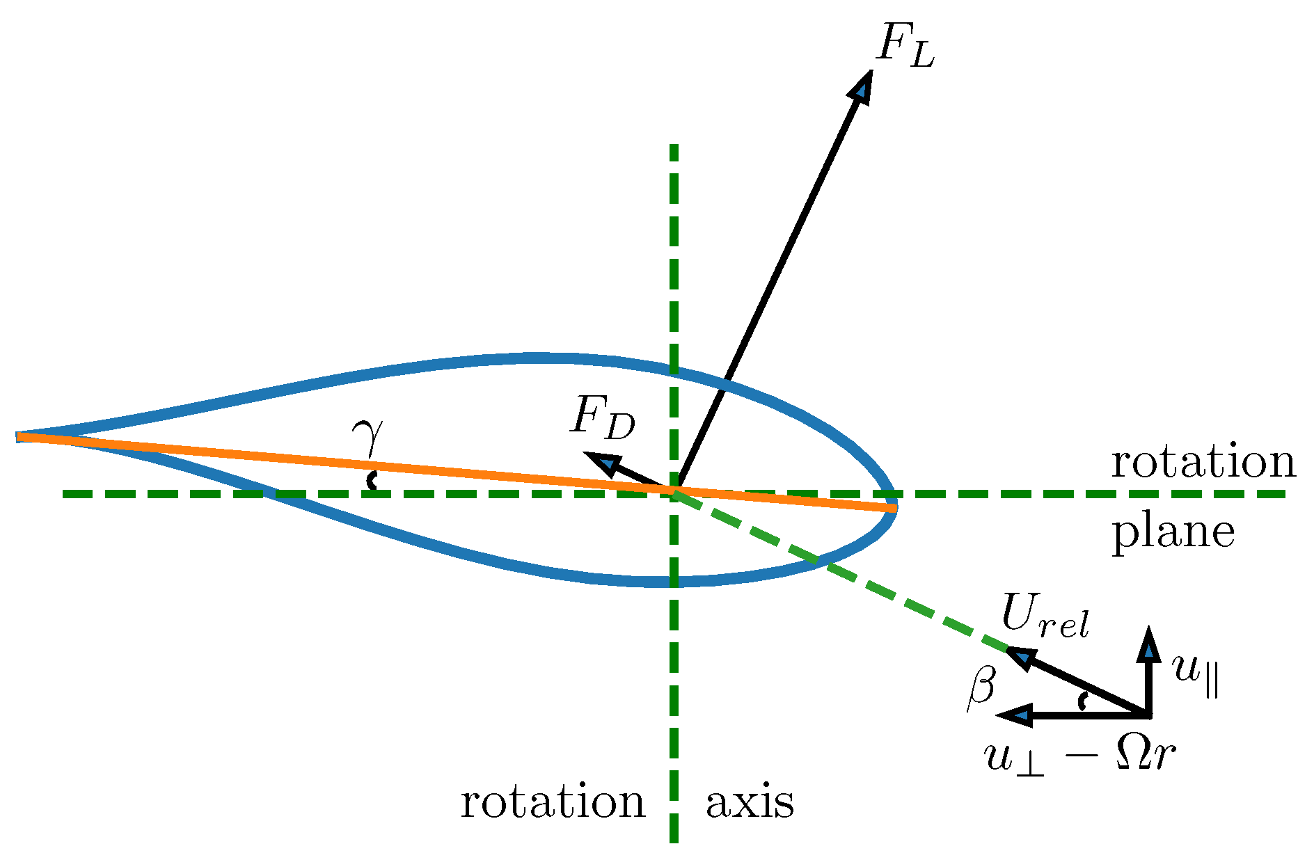
The actuator line model is used to calculate the turbine force exerting on the air flow. The blades are discretized into line segments from the blade roots to the tips. The aerodynamic lift force and drag force on each line element are evaluated based on the local relative flow velocity , empirical drag coefficient and lift coefficient , chord length c, and its length in the radial direction of the blades:
The empirical coefficients and are interpolated from their database based on the angle of attack , where is the twist angle of the airfoil section at the location of the line element, and is the angle between the relative velocity and the rotation plane, as shown in Figure 1.
The turbine is discretized on a Lagrangian mesh whose coordinate vector is time-dependent, while the fluid is discretized on a Eulerian mesh whose coordinate vector is time-invariant. The flow velocity at the Lagrangian coordinate X of a blade line element is evaluated from the velocity field on the background fluid grid. The aerodynamic force of a line element is the vector sum of and in Equations (9) and (10) and then distributed to the fluid grid as . We use the discrete Dirac function to project velocity from the background fluid to the blade grid points.
where the displacement vector is normalized by the grid size in the discretized domain, and is a smoothed version of the discrete Dirac function [18,36],
To project the force from the blade location to the fluid grid, we use the smoothed Dirac function when the grid is relatively coarse,
or the Gaussian kernel when the grid is fine enough to resolve the kernel width [22,37],
Here, is the number of blades and is the distance between the fluid grid point location and the i-th blade element location , of which the direction vector is . The influential ranges of summations for and are limited as the delta function and the Gaussian function vanish at large distances.
The nacelle and tower are discretized by triangular surface elements and their forces on the air flow are estimated following the idea of the immersed boundary method [38],
Here, the force recovers the flow velocity at the surface element to the desired velocity after a timestep . The coefficient for all the surface elements assures the drag coefficient for the bulk solid to be a preset value,
where is the undisturbed inflow velocity, A is the cross-sectional area of the structure (nacelle and tower), and is the unit vector in the inflow direction.
2.3. Treatment of Gibbs Phenomenon in Pseudo-Spectral Solver with Turbine Model
It is known that in spectral methods, the spatial discontinuity of a variable leads to unphysical oscillations called the Gibbs phenomenon. In the simulation of turbine wake flows, the existence of turbine force may lead to spatial jump for variables of interest, such as the pressure and velocity. To alleviate the Gibbs phenomenon due to the discontinuity around the turbine, modifications are needed for the spectral method.
The turbine force affects the Navier-Stokes equations as follows. There exists a jump in at the turbine location, which leads to a jump in through Equation (4) and a jump in through Equation (5). Then, the pressure p experiences a jump through Equation (7) and finally influences the updated velocity through Equation (6). The spectral method employed in the calculation of spatial derivatives, such as and , may produce unphysical oscillations if the jump is not well treated.
To alleviate the Gibbs phenomenon in the spectral solver, we propose a four-step scheme for the calculation of derivatives: identification, smoothing, derivation, and correction (ISDC). Previously, Li et al. [39] found that the numerical error from the discontinuity can be prevented from propagation to other regions of the computational domain if the discontinuity is smoothed before transferring the values to the right-hand side terms of the Poisson equation. They tested the effect of smoothing on the problem of flow past cube, where the spectral method was combined with the immersed boundary method (IBM). We extend their idea of smoothing to the ISDC scheme for the problem of flow past wind turbine, where the spectral method and ALM are combined. Among the four steps of ISDC, the identification step is to set flags for the location of discontinuity. In our code, the rotation of blades requires the identification at each time step. The flags are used to indicate the beginning and end of each segment of the discontinuous region. The smoothing step is to remove the discontinuity, which is described with an example later. The derivation step is to employ the classical spectral method for the computation of derivatives. Because the input of spectral derivation has been smoothed, the Gibbs phenomenon is alleviated. The correction step is to employ the finite-difference method for derivatives in the discontinuous region, which ensures the accuracy there. The new scheme is applied in all gradient calculations except for the pressure gradient in the Poisson equation. For the latter, a high-order smoothing is applied after the right-hand side term is transformed from the physical domain to the spectral domain [40].
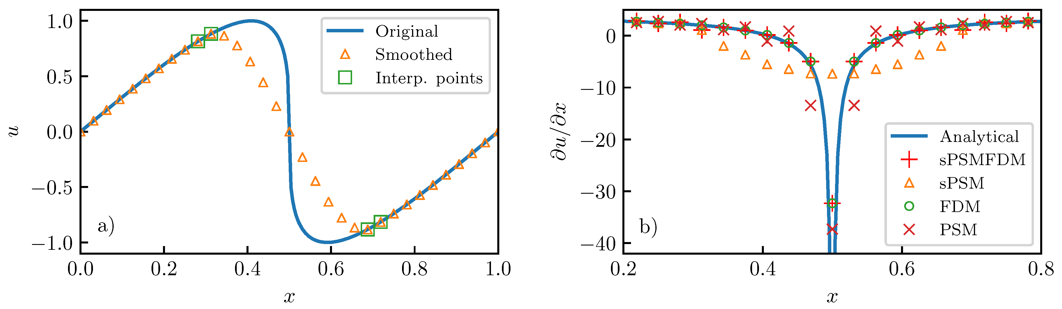
The new approach for derivative calculation is denoted as “sPSMFDM”, which means a combination of the smoothed pseudo-spectral method and the finite-difference method. The procedure of this hybrid approach is illustrated in Figure 2 with a test case of the one-dimensional inviscid Burgers equation. In the region where discontinuity occurs, the variable is interpolated with a cubic polynomial that has an effect of smoothing. Two points on each side of the discontinuous region are used to determine the coefficients in the cubic polynomial. After the interpolation and smoothing, the pressure field has less discontinuity and can be safely transferred to the classical pseudo-spectral method function. The output of the pseudo-spectral method (PSM) function should be highly accurate outside the discontinuous region. For derivatives inside the discontinuous region, the finite-difference method (FDM) is applied as a correction to the output from a smoothed input. As this FDM correction is needed only for a very small portion of grid points, the increment in computational cost is negligible. Our tests indicate that in the presence of discontinuity, the sPSMFDM provides derivative estimation with higher accuracy than classical PSM. A numerical test for sPSMFDM is provided in Appendix A.
3. Numerical Experiment
A numerical experiment is performed in the above-described LES-AL framework. The LES-AL code is modified from the LES framework described in [18,21,41,42]. The ALM part of the code is modified from the corresponding module in VFS-Wind, an open-source CFD code described in [20,43]. Similar LES-AL codes are described in [16,17,26].
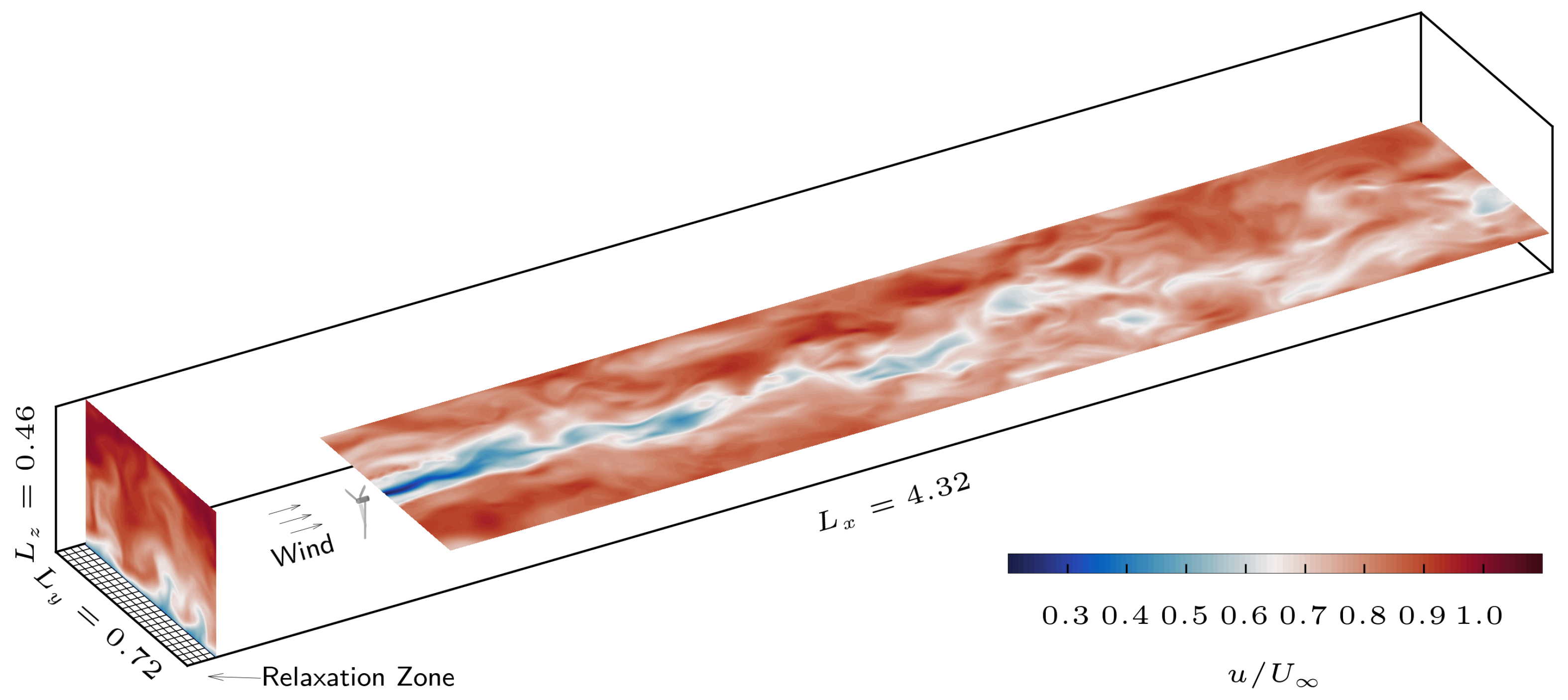
A miniature three-blade horizontal axis wind turbine is represented by actuator lines and placed in a numerical wind tunnel. The physical setup corresponds to the laboratory study performed by Chamorro and Porté-Agel [44], which was also adopted in other numerical studies [16,18,20,45] for method validation. The computational domain, as shown in Figure 3, has a size of , where the height is chosen based on the boundary-layer thickness reported in the experiment. The boundary condition for the streamwise velocity at the top is free-slip, , while the bottom boundary is non-slip, . A velocity relaxation zone [16,46] is used in the simulation to enforce an inlet boundary condition at the upstream. A precursor simulation, which develops to a statistically steady state without the turbine inside, provides a turbulent inflow of friction velocity m/s with surface roughness mm.
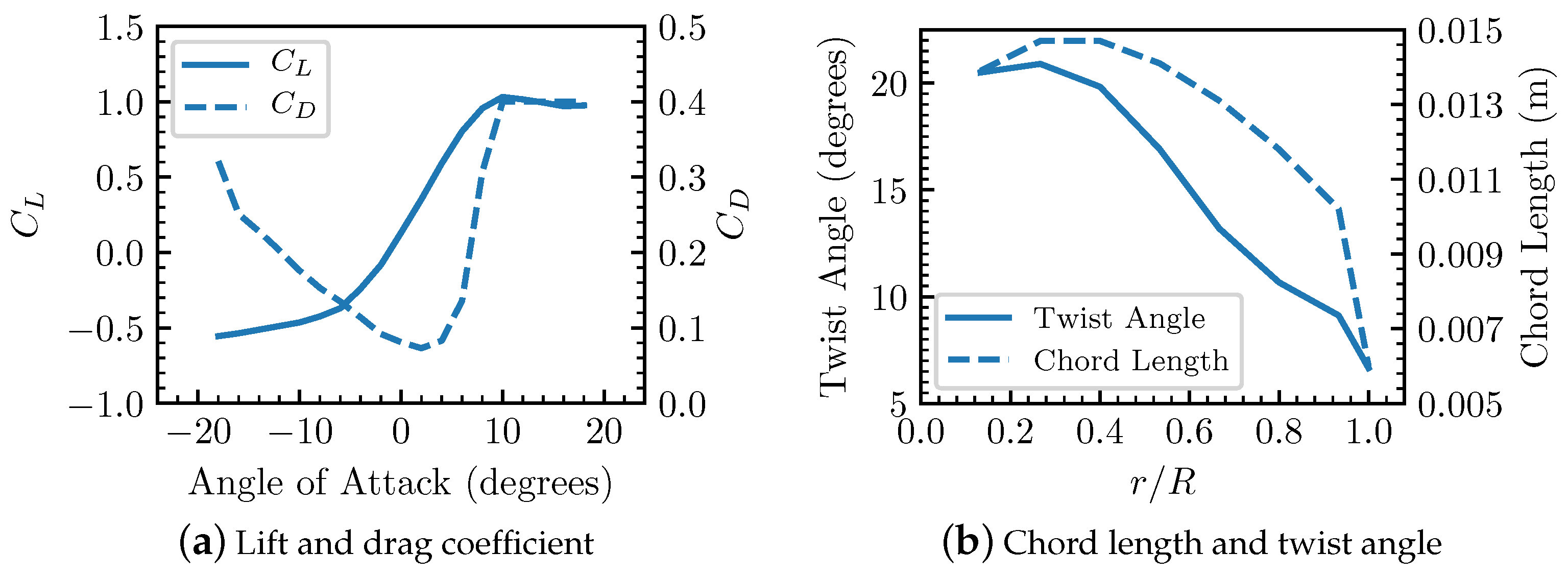
A three-blade miniature turbine, which has a blade diameter of m and hub height of m, is deployed at m, with corresponding to the inlet boundary. The actuator line parameterization for the turbine is set based on the prototype rotor GWS/EP-6030 [44]. The airfoil type along the entire blade is simplified as a circular arc airfoil. The lift and drag coefficients of the cambered airfoil at low Reynolds number are measured in the experiment by Sunada et al. [47] and provided in the simulation by Stevens et al. [26], as shown in Figure 4a. For angles of attack that are not listed in the experiment report, the aerodynamic coefficients are evaluated by theoretical formulas [48]
where is the drag coefficient at zero attack angle, and the threshold of small and high attack angle is adopted as the stall angle of the airfoil type. The chord length and twist angle at a normalized distance to the rotation center were obtained in the numerical study of Wu et al. [16], which are plotted in Figure 4b. The actuator line elements start from the radial distance m, while in the inner region m the nacelle model takes effect following Equation (15). Below the nacelle, the tower is assumed to be a vertical cylinder of diameter m and length m. The tower drag is considered in the same way as the nacelle drag. The drag coefficients of the nacelle and tower are 1.5 and 0.8 respectively, which are set based on the empirical ranges and our tests to acquire a best fit of the mean velocity profile in the near wake at compared to the experiment measurement. A constant rotation speed of the turbine rotor is determined based on a tip-speed-ratio of and the hub mean flow velocity m/s.
The computational domain is discretized on a structural Cartesian mesh of cells. The grid number is refined from a previous simulation by Porté-Agel et al. [17] in the same physical domain, which adopted a similar spatial scheme with ours in a coarser mesh of and achieved plausible accuracies in both the mean velocity and turbulent intensity profiles. The first off-wall grid point is located at . The shear stress at the bottom are obtained following Equation (8). The grid is stretched in the vertical direction so that it is denser in the rotating region. The blade diameter is covered by about 24 grid points in the vertical direction, which is refiner than 20 grid points per diameter as recommended by Yang et al. [20] for the simulation of the same experiment. Each blade is discretized into 40 segments with a resolution refiner than the fluid mesh. The nacelle and tower are represented by triangular surfaces. The grid of the fluid domain and the turbine structure are shown in Figure 5. The simulation runs with a constant time step , where T is the period of turbine rotation. After the bulk flow advects in the streamwise direction for one cycle of the domain, the simulation continues running for to perform statistical analyses for the turbine wake flow.
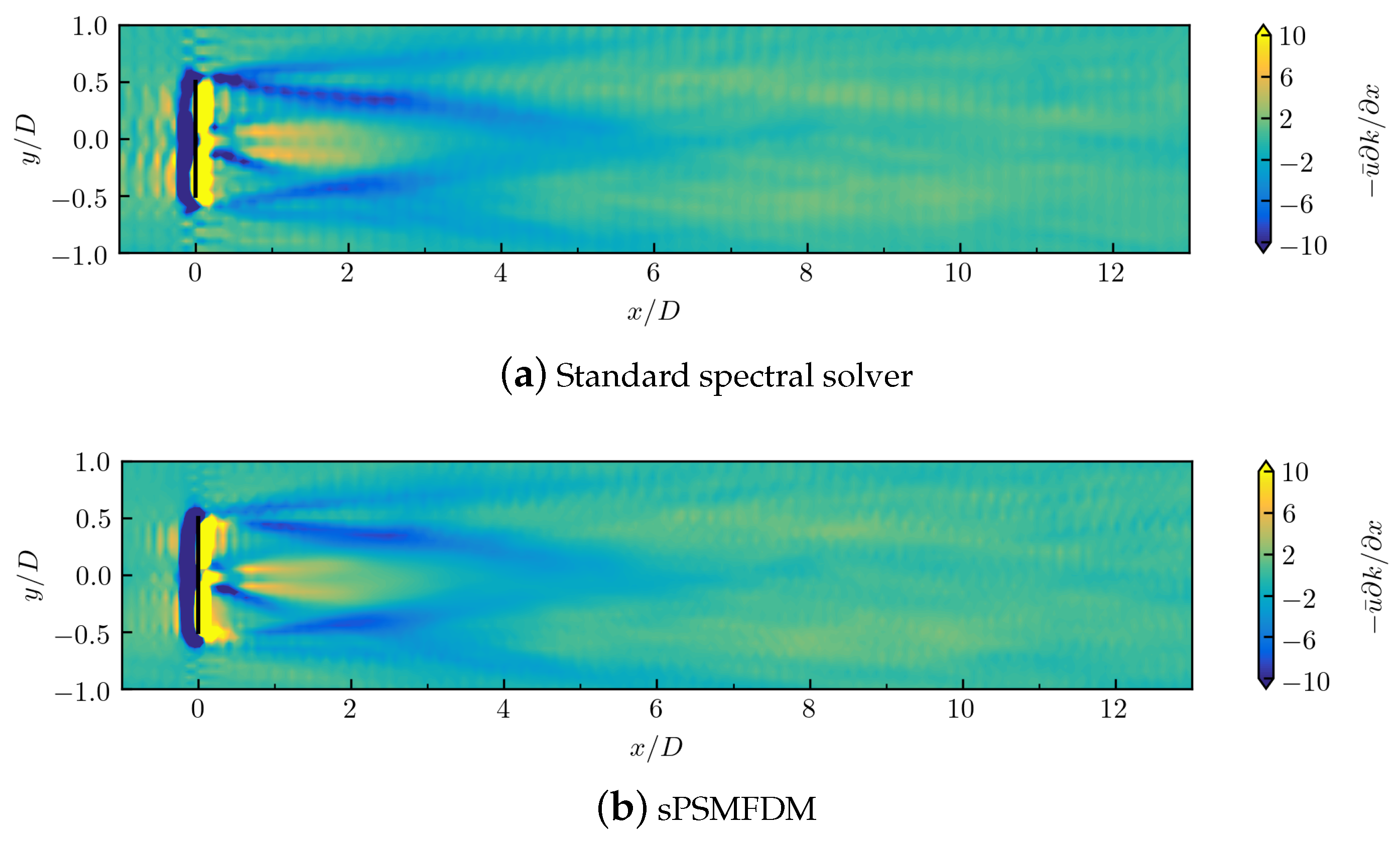
The proposed method sPSMFDM is applied in the simulation to alleviate the Gibbs phenomenon. As pointed out by Martínez-Tossas et al. [37], there is an optimal smoothing length scale for ALM, which is around 14%–25% of the chord length of the blade. This optimal smoothing length scale is smaller than our averaged grid size. To make our smoothing width closer to the optimal value, we used the three-point discrete Dirac function in Equation (12) which results in the Gibbs phenomenon if a standard PSM is used for the calculation of the spatial derivative. The numerical oscillations can be observed in the distribution of the spatial derivatives, such as the streamwise advection of the turbulent kinetic energy (TKE, ) shown in Figure 6a. After applying the proposed special numerical treatments in Section 2.3, the numerical oscillations are alleviated in the wake region of the domain, as shown in Figure 6b. It should be noted that there are three types of spectral operators in the code, namely the spatial derivative operator, the dealiasing operator, and the spectral solver for pressure. The special treatments introduced in Section 2.3 take care of the first and the second spectral operators, while the spectral solver for pressure is unchanged. Therefore, instead of totally eliminating the numerical oscillations, the special treatments in this study alleviate the numerical oscillations and restrain the remained oscillations to a smaller region in the very near wake. The treatment for the spectral pressure solver is to be studied in future.
4. Results and Discussion
4.1. Validation of the LES Coupled with the Actuator Line Model and Nacelle Model
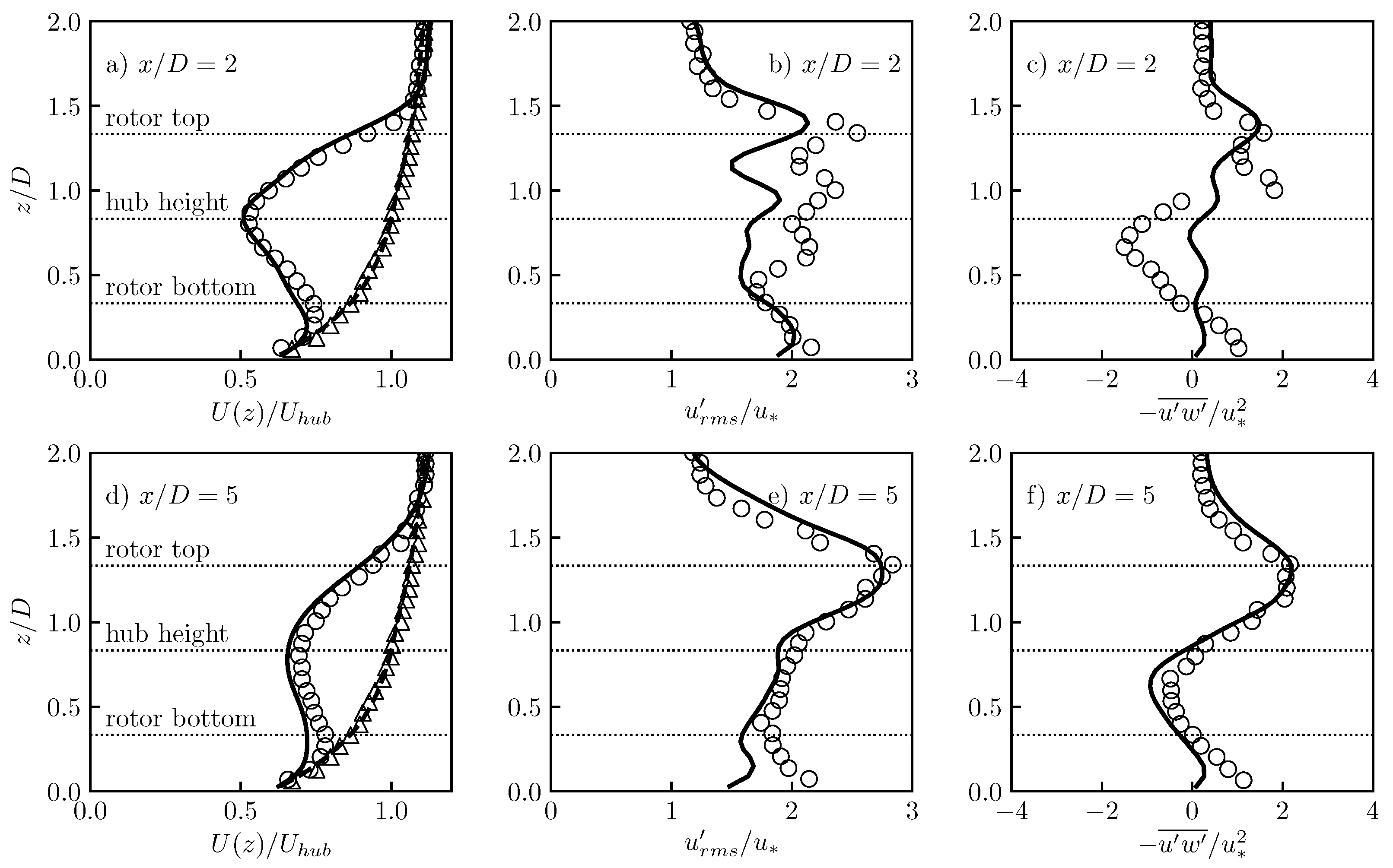
The time-averaged profiles of velocity, turbulence intensity, and Reynolds stress at and downstream of the turbine are shown in Figure 7. In Figure 7a,d, the mean velocity profiles of our simulation agree well with the wind-tunnel measurement [44]. The influence of turbine forces is reflected by the mean velocity deficit as compared to the undisturbed upstream flow. The initial deficit in the vicinity of the turbine is caused by the energy extraction of the blades and the drag of subsidiary structures such as the nacelle and tower. As the distance to the turbine increases, the velocity deficit decays. In Figure 7b,e, the turbulence intensity profiles of our simulation show similar trend as the measurement data. The magnitude of turbulence intensity in simulation is smaller than that of wind-tunnel measurement, which is not surprising as the large-eddy simulation does not resolve all scales of the turbulence [25]. The peak of turbulence intensity at the rotor top contains the contributions of tip vortex and large vertical gradient of the mean velocity, while the turbulence intensity at the rotor bottom is less or equal to that of the inflow due to negative or small velocity gradient [49]. In Figure 7c,f, the Reynolds stress profiles of our simulation also show similar trend as the measurement data. The simulation profiles of turbulent components are closer to the measurement at than at .
In summary, the simulation predicts the mean velocity accurately and reproduces the turbulence properties reasonably well. In the following sections, more flow characteristics are presented from the simulation data.
4.2. Self-Similarity in Mean Velocity
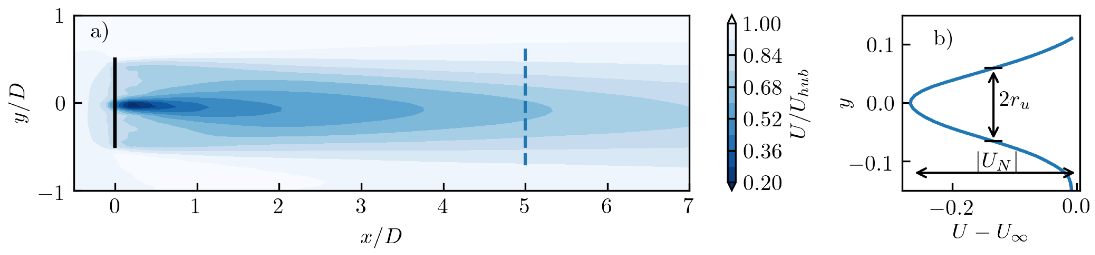
Self-similarity is widely observed in free shear flows such as mixing layer and plane jet. Because the rotation region of turbine blades is a circular disk, the wake of turbine may conform to the theory of axisymmetric wake. In the vertical cross-section, the planar boundary layer where the turbine sits introduces asymmetry to the wake flow. On the other hand, the wake flow in the horizontal cross-section remains symmetry along the centerline, as shown in Figure 8a.
In classical boundary-layer theories, the mean velocity in far wake is assumed to satisfy the trial function [2]
where is the characteristic velocity difference. The original meaning for the subscript “N” might be “negative”. In this study, “N” indicates that the variable is a characteristic scale used for “normalization”. is the characteristic width of the spanwise distribution of velocity deficit, and is the non-dimensional spanwise distance. The trial function separates the velocity deficit to contributions from streamwise distance x and normalized spanwise distance , respectively. For a turbulent axisymmetric wake, the spanwise distribution of velocity deficit is close to the Gaussian distribution, as shown in Figure 8b. The maximum deficit at each streamwise distance x is chosen as the characteristic velocity difference. The half width where the velocity deficit decays to is denoted as , which can be chosen as the characteristic length in the spanwise direction.
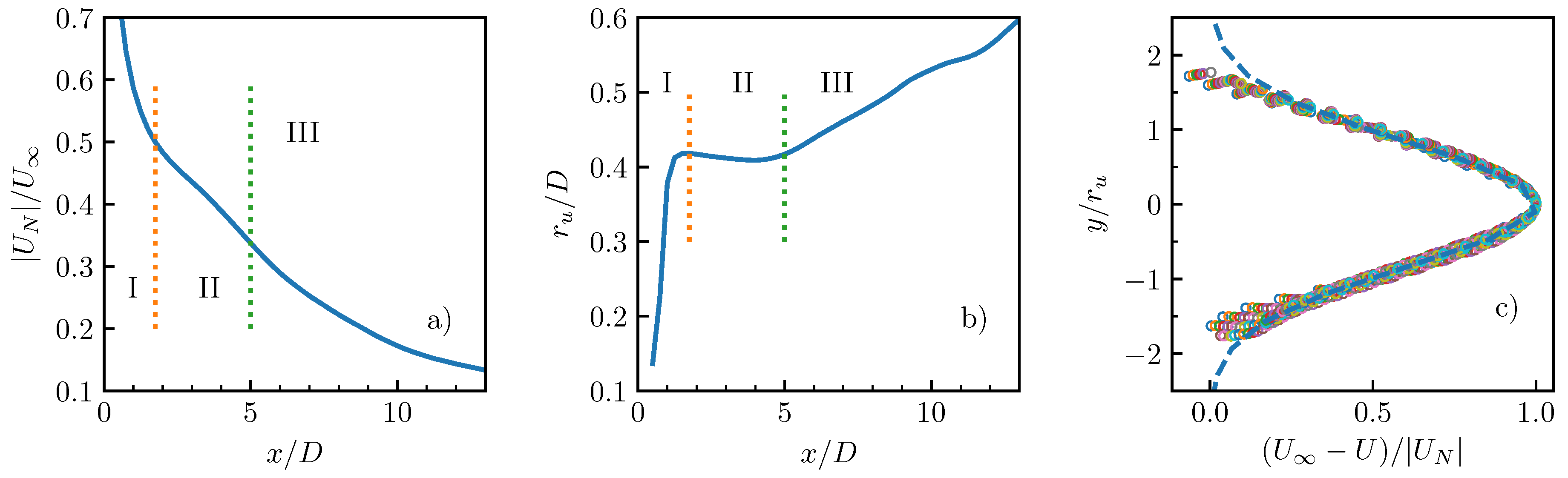
The self-similarity of the mean velocity is manifested after normalization by the characteristic length and velocity difference . The maxima of velocity deficit are located around the centerline stretching from the turbine hub to downstream. As shown in Figure 9a,b, the velocity deficit maximum decays with the streamwise distance x while the half width grows with x. If the velocity deficit and spanwise distance y are normalized by the velocity deficit maximum and half width , respectively, the spanwise distributions of the mean velocity deficit collapse, indicating the occurrence of a self-similarity.
The streamwise development of the self-similarity is categorized into three stages based on the characteristic scales and the normalized velocity profiles. The thresholds of these stages can be determined from the changes of the growth rate of the half width . The thresholds can also be confirmed by the decay rate of the velocity deficit maximum . Three stages are separated by the dotted lines in Figure 9a,b. Stage I in is the near wake region, where the velocity deficit profile does not fit a Gaussian distribution, meaning that the flow has not entered the regime of self-similarity yet. The normalized velocity profiles of stage II at and stage III at fit the same Gaussian distribution in the spanwise direction, as shown in Figure 9c. Therefore, stages II and III are in the regime of self-similarity for the mean velocity. However, the change of growth rate at indicates that an incident happens there. In the literature review of Xie and Archer [30], another three-stage categorization was mentioned: the near wake, the transition region, and the far wake. The locations of the boundaries of the stages are similar between these two categorizations. To clarify, our categorization is based on the quantitative analysis of the characteristic scales. The second stage of our categorization is not a “transition stage” as the self-similarity is observed. The mechanisms behind the establishment and development of the self-similarity are explained in Section 4.4 and Section 4.5.
4.3. Self-Similarity in Reynolds Stress
The Reynolds stress plays a vital role in the evolution of mean velocity field in the turbulent wake flow. With a similar process of defining the characteristic scales and normalizing afterwards, the self-similarities are also found for the Reynolds stress components and in the horizontal plane at the hub height.
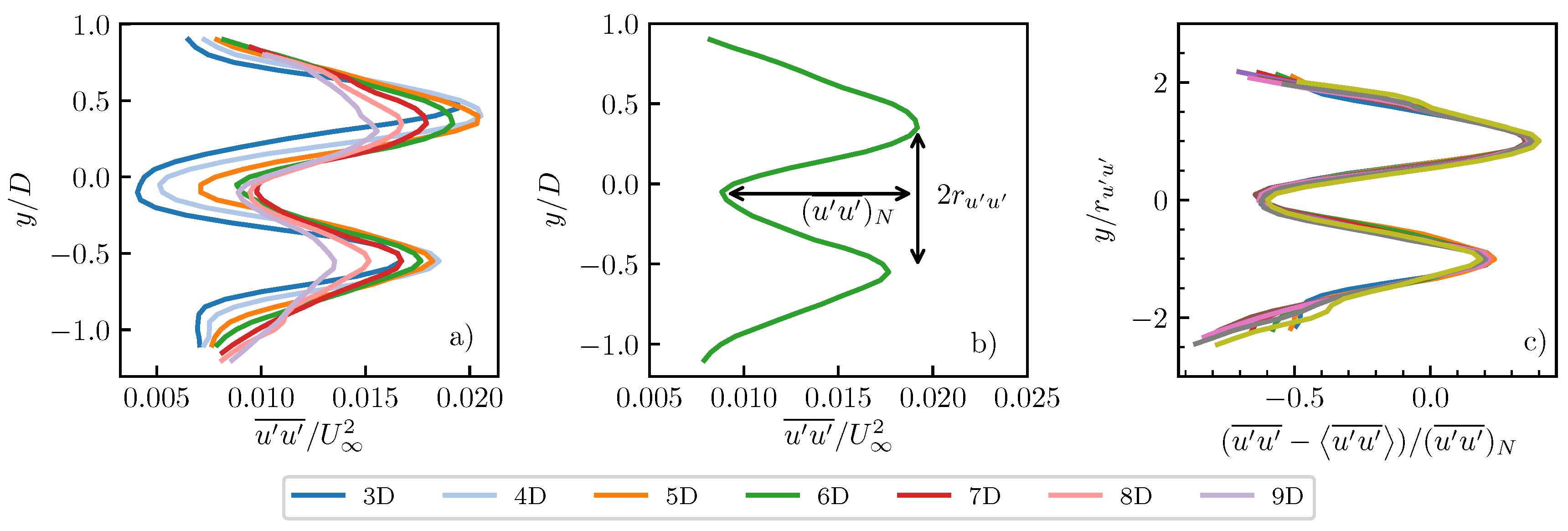
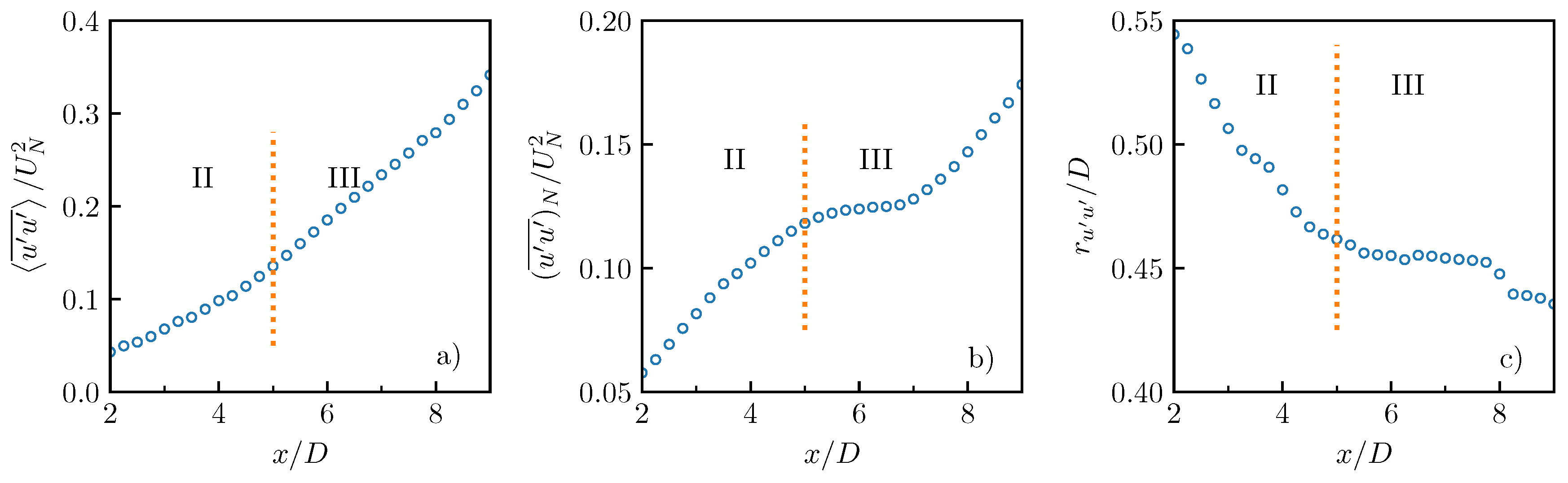
For the Reynolds stress component , the general shape of its spanwise distribution in the stages II and III is shown in the normalized profile in Figure 10b. It has two peaks at and a trough at . The characteristic Reynolds stress scale is defined as the difference of between the peak and the trough, while the characteristic width scale is defined as half of the spanwise distances between the two peaks. The normalized profiles of in the region well collapse to the same curve, as shown in Figure 10c. For the region surrounding but outside , the normalized profiles are in a similar shape but with some deviations. A subtraction of the spanwise averaging between the two peaks, , is necessary in the normalization to achieve the collapse. The normalized Reynolds stress in the side is a bit larger than that in the side . For the streamwise development of the characteristic scales, as shown in Figure 11, a change of the tendency is observed at the boundary of the stages II and III. The length scale , namely the spanwise peak-to-peak distance, stays at a flat level after entering the stage III.
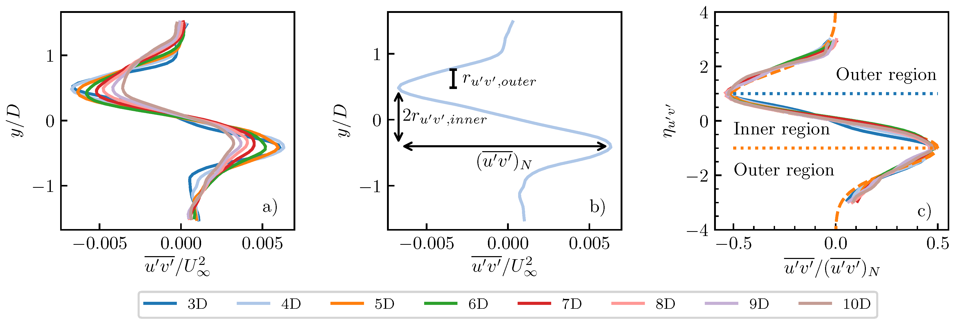
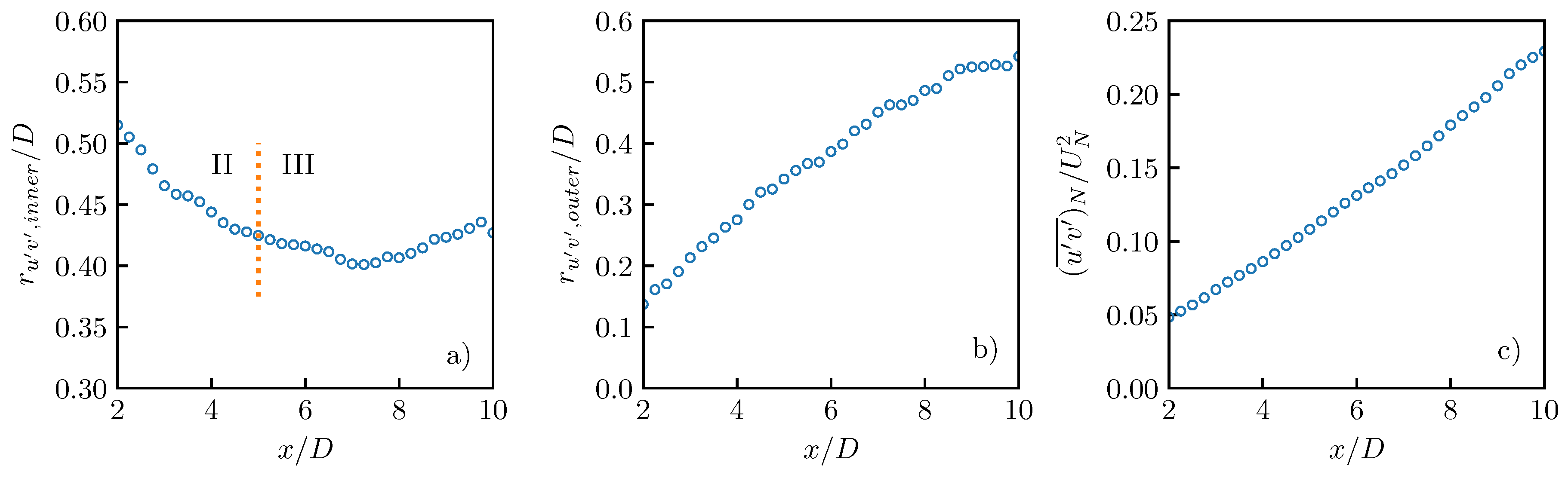
For the Reynolds stress component , its general shape of the spanwise profile is shown in Figure 12b. Two different characteristic width scales are found inside and outside the peak/trough pair, respectively, by which an inner region and an outer region are separated. For the inner region, the characteristic Reynolds stress and the characteristic width are defined as the spanwise distance and the Reynolds stress difference, respectively, between the pair of peak and trough. For the outer region, the characteristic width is defined as the distance to the peak/trough where the Reynolds stress decays to a half. As shown in Figure 12c, the normalized profiles of in the region well collapse to the same curve. Derived from the boundary-layer equation shown in Equation (23), the normalized profile of has an analytical solution
where is the normalized spanwise coordinate defined as below,
The streamwise development of the characteristic scales is shown in Figure 13. The entry of the stage III causes a noticeable change of tendency only in the inner width scale.
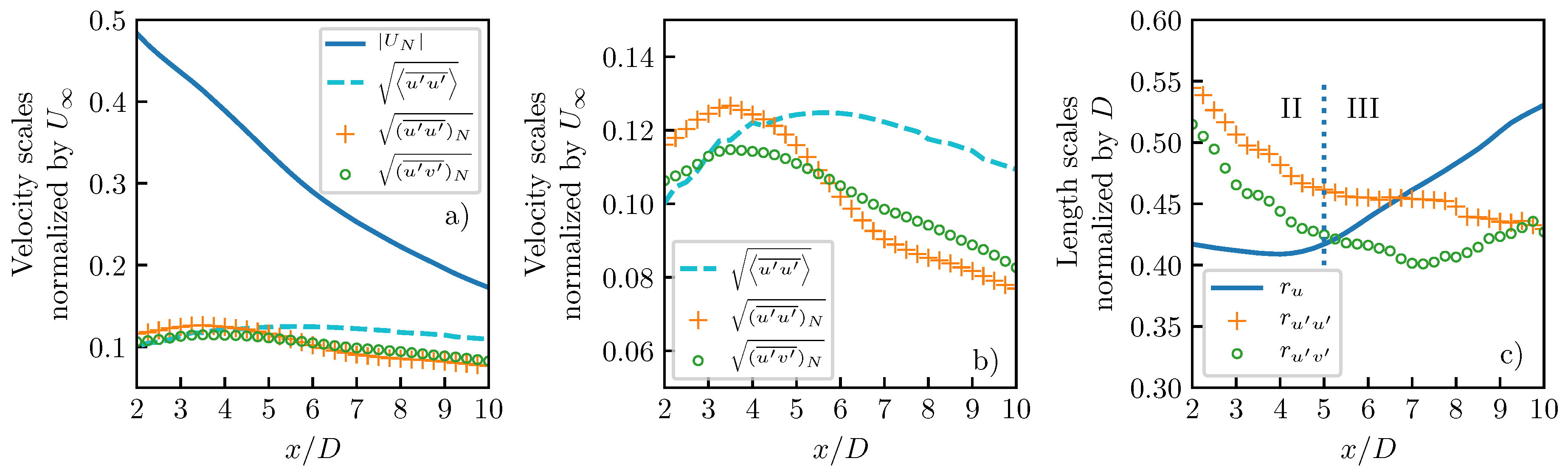
The spanwise gradient of the mean velocity is assumed to be the source of the turbulent kinetic energy (TKE) in the turbine wake. Therefore, the mean velocity deficit scale is used in the normalization of the Reynolds stress scales in Figure 11a,b and Figure 13c. The -normalized Reynolds stress scales show nearly linear dependence with the streamwise distance, which supports the assumption of TKE source. As is decreasing with x, the absolute trends of the Reynolds stress scales are more complex than a linear relation. The comparison of four velocity-like scales , , and are shown in Figure 14a,b. By normalization with a x-irrelevant parameter , the Reynolds stress scales grow at the starting stage and decay afterwards. The comparison of three length scales , , and are shown in Figure 14c. In stage III, the widths of and are at a stable level, while the width of velocity deficit keeps growing.
4.4. Mean Momentum Equation and Boundary-Layer Equation
With certain assumptions and simplifications to the Navier-Stokes equations, the boundary-layer equations provide theoretical solutions for boundary-layer flows. The self-similarities occur after a development stage, which is a long distance from the static axisymmetric body. Johanasson and George [50] reported that in a disk wake flow of Reynolds number , the self-similarity starts from for the mean velocity and for the turbulent intensity. Uberoi and Freymuth [51] reported that in a sphere wake flow of Reynolds number , the self-similarity starts from . In our simulation, the self-similarity of streamwise velocity starts from and the self-similarity of Reynolds stress starts from at a Reynolds number of , which has a comparable Reynolds number but at a shorter distance. Although the earlier occurrence of the self-similarity in the turbine wake is a bit surprising at first glance, it can be explained by a budget analysis of the mean momentum equation.
In the cylindrical coordinate system , the continuity equation is
The mean momentum equation on cylindrical coordinates is
The terms on the left-hand side of Equation (22) are the mean flow convections. The last three terms on the right-hand side are effects of the Reynolds stress. In axisymmetric wakes, firstly the terms containing derivatives with respect to angle diminish due to the symmetry. Secondly, in turbulent flows, the terms containing molecular viscosity are neglected as they are smaller than the terms containing the turbulent viscosity . Thirdly, the pressure gradient is assumed to be small in the self-similarity regime that is far away from the body. Lastly, , the streamwise derivative of Reynolds stress, is neglected because it is much smaller than the radial derivative term .
Based on the considerations above, a simplified mean momentum equation is obtained as
To close the equations, the turbulent viscosity and mixing-length model are used to estimate the Reynolds stress term in Equation (23) [2],
where is the turbulent viscosity for the axisymmetric wake and is a non-dimensional constant for the turbulence.
The classical solution to the boundary-layer Equations (21) and (23) is [2]
where is the drag coefficient of the axisymmetric body, is the dimensionless expansion rate for the wake width , and is the virtual starting location of the self-similarity. The relation between and is . The classical solution assumes that
where is a x-independent parameter. As a result, the boundary-layer Equation (23) is simplified to an equation of the dimensionless coordinate , and the self-similarity is obtained.
The solution of the mean velocity predicts that
Equation (30) indicates that the boundary-layer Equation (23) yields a Gaussian distribution of the mean streamwise velocity in the radial direction.
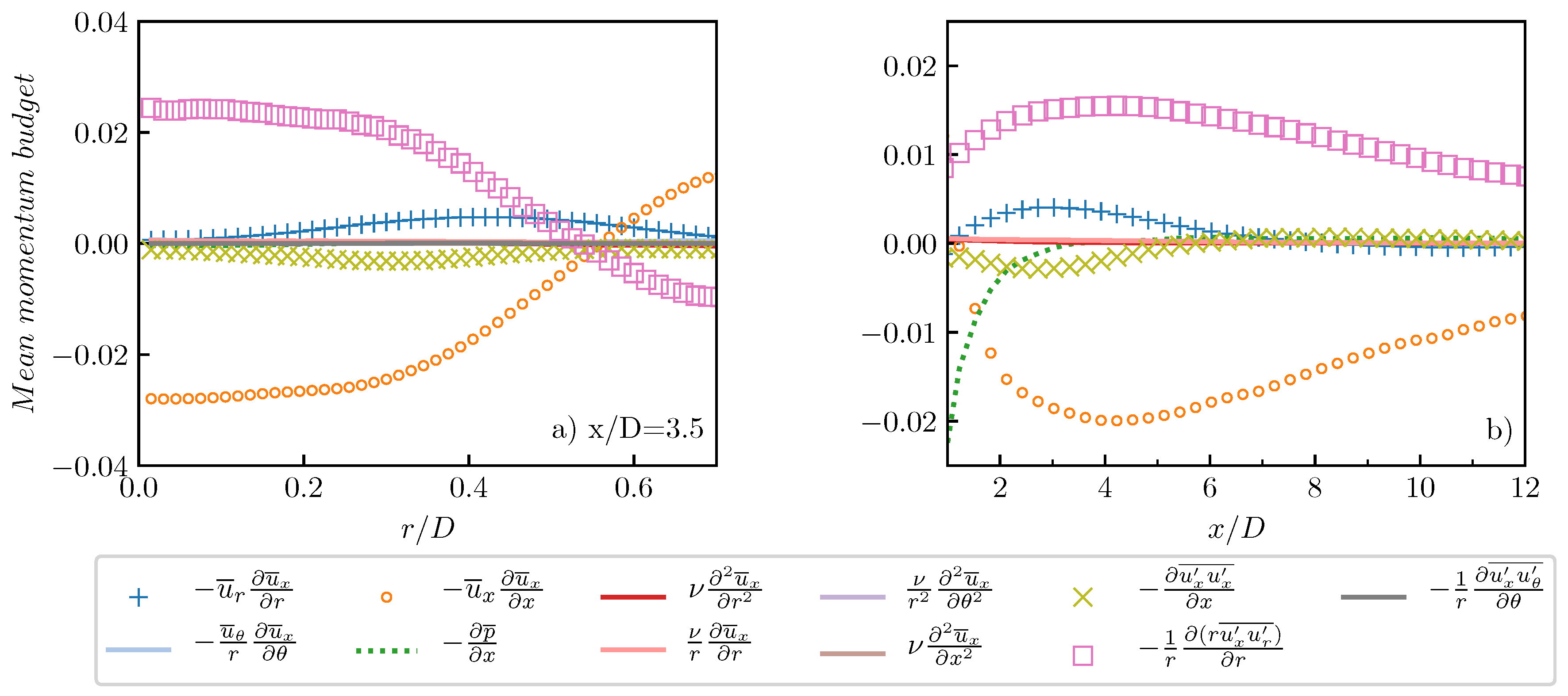
The derivation of the Gaussian distribution for the streamwise mean velocity helps us understand the self-similarity shown in Figure 9c. However, considering the planar boundary layer and the rotation effect, the turbine wake is not a purely axisymmetric flow. The assumptions in the simplification of the momentum equation should be verified for the turbine wake flow, which can be done by examining the mean momentum budgets of Equation (22) using the LES data. A temporal averaging is firstly performed at each grid point. Next an azimuthal averaging is performed to acquire the temporal-radial mean field. Figure 15a shows the radial distribution of each mean momentum budget term at , which is the center of stage II of the self-similarity. By further applying a radial averaging with the radius as the weighting function, the temporal-azimuthal-radial averaged momentum budget is acquired. As shown in Figure 15b, the dominant terms in the budget of mean momentum are the radial turbulent production term and streamwise convective destruction term . The radial convective production term is the third dominant term, which is smaller than the other two leading terms in the region and becomes negligible in the region . The fourth dominant term is the streamwise turbulent destruction term , which contributes a small fraction of mean momentum in the region . The pressure gradient term is important in the region and becomes negligible in the region .
By overlooking the development of the mean momentum budget terms in the streamwise direction as shown in Figure 15b, it could be found that the leading terms in stage II and III are the streamwise convection term , the radial derivative of Reynolds stress term , and the radial convection term .
The leading terms in the mean momentum Equation (22) can also be confirmed by simple calculations based on the self-similarity and the characteristic scales analyzed in Section 4.2 and Section 4.3. For the streamwise convection term in the region , the mean velocity is estimated as , which is the difference of the inflow velocity and the averaged velocity deficit scale . The derivative is estimated as , with the gradient read from the slope at and in Figure 14a. The estimation process is reorganized as below,
Other three leading terms found in Figure 15 can be estimated in a similar approximation, as shown below,
Here, these four terms are estimated using data in the region . In the estimation of the third term , is the scale of the radial mean velocity . The scale is defined as the maximum radial mean velocity at a downstream distance x. In the region , changes from to as x increases. As the radial velocity scale is one order smaller than other velocity-like scales, its development along x contains a lot of noises. Thus, it is not shown as other variables of interests.
Compared to the cylindrical averaged results in Figure 15, the characteristic scale-based estimation above provides the same sequence of importance for the terms in the mean momentum budget,
The fourth term is one order smaller than the third term. The third term is nearly one order smaller than the leading two terms, which makes the leading two terms seem to balance with each other. By ignoring the small terms, three leading terms constitute to the boundary-layer Equation (23), which has a Gaussian solution (30) based on past studies of classical axisymmetric wake. Therefore, it is not surprising to observe that the self-similarity occurs as early as behind the turbine, compared to the starting point in classical axisymmetric wake at a similar Reynolds number.
The mean momentum budget analysis also throws light on how to get more accurate theoretical solutions for the mean flow of turbine wake. At stage I (), the pressure gradient and streamwise convection are the dominant terms. At stage II (), the consideration of streamwise turbulent destruction in the boundary-layer equation should give a better solution. In region of stage III, the boundary-layer Equation (23) could be further simplified to a two-term equation where the radial convection is neglected.
4.5. The Collision Hypothesis of Wake Meandering and Tip Vortices
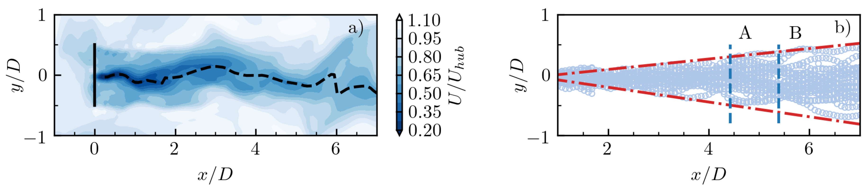
Under the perturbations from the turbulent flow upwind, the wake flow of a turbine has a transverse meandering with strong interactions between the wake flow and the ambient flow. The velocity deficit centerline is often used to represent the motion of wake meandering [12,31]. At each streamwise location, the spanwise coordinate of the wake centerline is identified with the velocity minimum in the transversal cross-section. A spanwise averaging window is applied in the search of the velocity minimum to reduce fluctuations. As shown in Figure 16a, the centerline originates from the turbine hub and extends downstream with a gradually increasing spanwise amplitude. By superposing the wakelines at various times in the simulation, the region where the low-speed wake sweeps is acquired, as shown in Figure 16b. Some extreme samples of the wake meandering are filtered out, which leaves the coverage map with a pair of smooth edges. In our simulation, the expansion angle of the wakeline is .
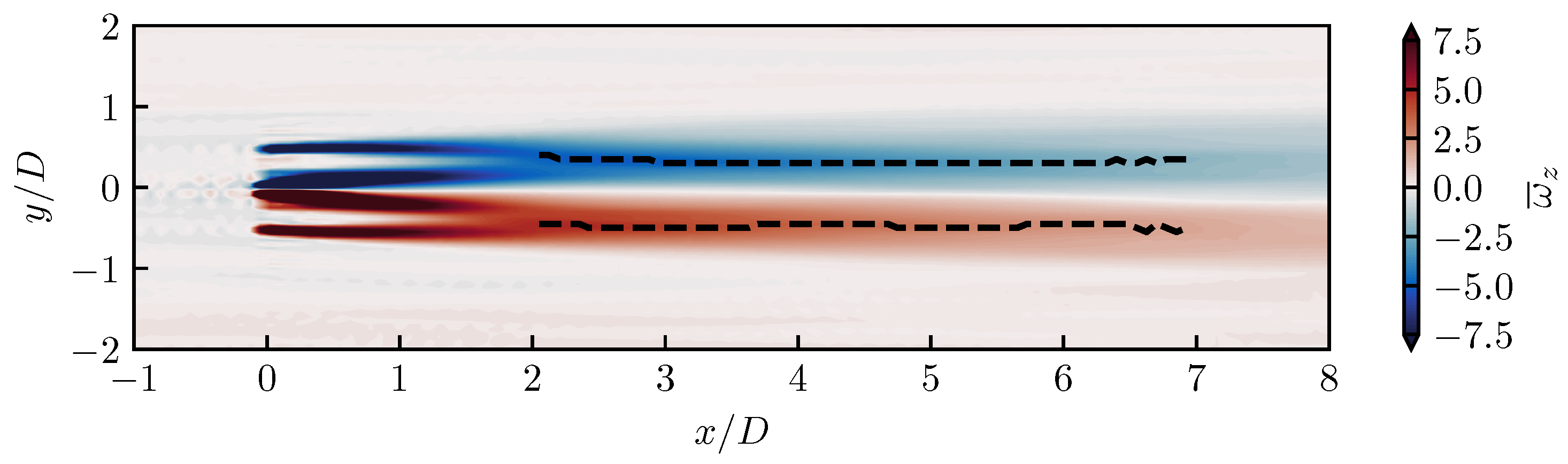
Tip vortices are another source of turbulent kinetic energy in the wake flow. They are convected downstream under the influences of the ambient flow in the outer region and the velocity deficit in the inner region. Howard et al. [12] assumes that tip vortices move along , which corresponds to a width of D between tip vortices in a horizontal slice crossing the hub. The spanwise velocity around the tip vortex is simplified as zero in the assumption of [12]. However, as the wake expands downstream, the spanwise velocity should point to the central axis to entrain the ambient flow. Considering the continuity Equation (21) and the decreasing gradient of the streamwise velocity along x, the amplitude of spanwise velocity around the tip vortex should also decrease with x. Consequently, the tip vortices may have a small inward displacement due to the spanwise velocity of the flow. The inward displacement may have a limit as the amplitude of spanwise velocity decays with x. Hu et al. [52] presented the evolution of the unsteady vortex in turbine wake with phase-locked PIV measurements. Although they did not state explicitly, the inward displacement of tip vortices could be observed in the scattering of the wandering tip vortices. Based on the analyses above, the width of tip vortices may be smaller than the rotor diameter D. By assuming the tip vortices are located at the positive and negative peaks of the vertical vorticity in the horizontal plane at the hub height, the width of tip vortices could be estimated from the mean vorticity field in the simulation. As shown in Figure 17, the width W in region is at a steady value .
Given the expansion rate of the velocity profiles and the nearly constant width W of the tip vortices, the collision of these two flow structures is expected to occur at downstream location. As shown in Figure 16b, the collision location is estimated to be for or for .
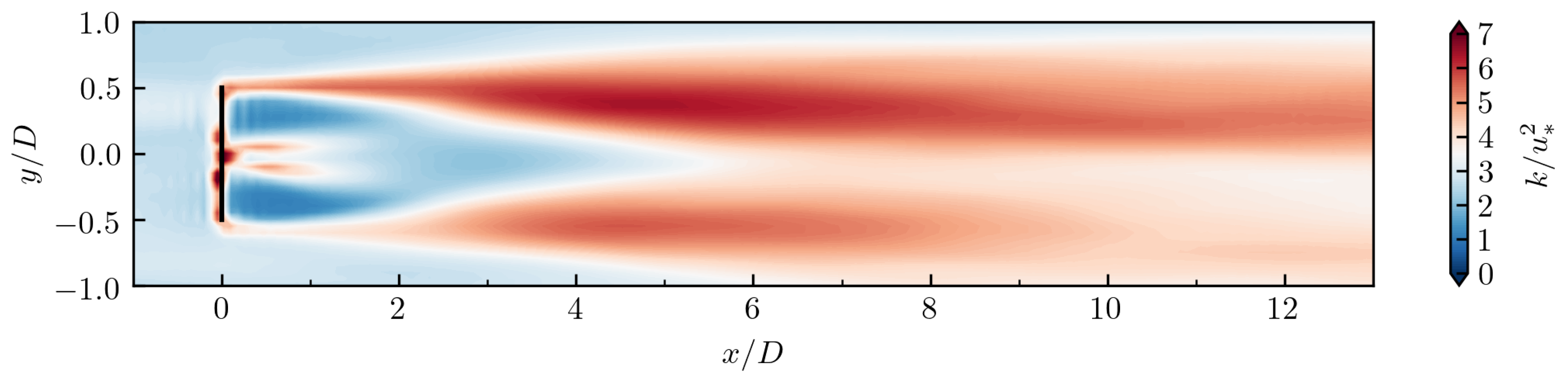
The development of TKE also discloses the interactions in the wake flow of turbine. As shown in Figure 18, strong TKE k is observed at , around the estimated location of the collision shown above. The collision leads to generation of TKE. The Reynolds stress is enhanced due to the collision. This further leads to a larger turbulent viscosity in Equation (24), a larger dimensionless turbulence parameter in Equation (25), and a larger in Equation (28). Noted that is the dimensionless expansion rate of the wake width in Equation (27), there is thus a larger growth rate of half wake width in Figure 9. As the collision position is located at the boundary of stages II and III of the self-similarity, , the interaction between the meandering velocity deficit and the tip vortices leads to the transition from stage II to stage III.
The asymmetry is observed in the distribution of TKE. In two previous experiments, the asymmetry was also observed in either the turbulent intensity [44] or the wake expansion angle [12]. In those experiments, the turbine GWS/EP-6030 rotates along direction and the activity of interest is stronger in . In our simulation, we set the turbine to rotate along direction and the activity of interest is stronger in . Therefore, the asymmetry might be caused by the rotation of the turbine blades. In Figure 10 and Figure 12, the normalized profile of shows an asymmetry while does not.
5. Conclusions
In this study, the wake flow of a model-scale wind turbine is investigated by LES. A hybrid derivative approach sPSMFDM is proposed to alleviate the Gibbs phenomenon in the simulation using the spectral method and the actuator line model. The self-similarity of mean velocity in the turbine wake and its mechanism are investigated. The following conclusions are obtained:
The Gibbs phenomenon can be alleviated by the sPSMFDM approach, which smooths the input of the PSM and rectifies the output by the FDM. The accuracy of the simulation is validated through comparisons of flow statistics to wind-tunnel measurements.
By defining the maximum velocity deficit and the half velocity profile width as the characteristic scales of velocity and length, respectively, the self-similarity of mean velocity is illustrated. Based on the development of the self-similarity, a new three-stage categorization of the turbine wake is proposed. Stage I is the developing near wake. The self-similarity starts in stage II where the normalized velocity profiles collapse to the same Gaussian distribution in the spanwise direction. Stage III also obtains the self-similarity, while the expansion rate of wake becomes larger than at stage II. The self-similarities of the Reynolds stresses and in the turbine wake are investigated for the first time. The normalized spanwise profiles of the Reynolds stresses collapse to the same curves after defining the characteristic scales properly. The theoretical formula for the normalized is provided.
The mechanisms in the establishment and the development of the mean velocity self-similarity are discussed. A mean moment budget analysis is performed using the cylindrical averaging and the characteristic scale-based estimation. The budget analysis shows that, the leading terms affecting the mean momentum are the streamwise convection and the radial gradient of Reynolds stress. It confirms the assumptions in simplifying the boundary-layer equation for the axisymmetric wake. The Gaussian solution of the simplified BLE is the mathematical basis for the self-similarity in the mean velocity starting at stage II. By recalling the condition in the derivation of self-similarity solution. The increment of the turbine wake expansion rate at the boundary between stage II and III is explained. At that boundary, the collision of the tip vortices and the meandering wake deficit enhances the turbulence. The condition in the derivation of the self-similarity indicates that the enhanced Reynolds stress at the collision leads to the increment of the expansion rate of the turbine wake.
Author Contributions
Conceptualization, P.L., H.L., and L.S.; Methodology, P.L. and L.S.; Software, P.L. and L.S.; Validation, P.L. and L.S.; Analysis, P.L.; Writing—Original Draft Preparation, P.L.; Writing—Review & Editing, W.-L.C., H.L. and L.S.; Supervision, H.L. and L.S.; Project Administration, H.L. and L.S.; Funding Acquisition, P.L., W.-L.C. and L.S.
Funding
This research was funded by the National Natural Science Foundation of China (NSFC, No. 51722805), the China Scholarship Council (CSC, No. 201606120186), and Xcel Energy’s Renewable Development Fund (RDF, grant HE4-3). The authors are grateful for the supports.
Acknowledgments
The authors acknowledge the Minnesota Supercomputing Institute (MSI) and St. Anthony Falls Laboratory (SAFL) at the University of Minnesota for providing the computing resources that contributed to the research results reported within this paper. The authors also acknowledge the computing resources provided by the National Supercomputer Center in Guangzhou (NSCC-GZ).
Conflicts of Interest
The authors declare no conflict of interest.
Abbreviations
The following abbreviations are used in this manuscript:
| AB2 | Second-order Adams-Bashforth scheme |
| ADM | Actuator disk model |
| ALM | Actuator line model |
| BEMT | Blade element momentum theory |
| FDM | Finite-difference method |
| IBM | Immersed boundary method |
| ISDC | Identification, smoothing, derivation, and correction |
| LES | Large-eddy simulation |
| LES-GR | Geometry-resolved LES |
| LES-AL | LES with ALM |
| PIV | Particle image velocimetry |
| PSM | Pseudo-spectral method |
| sPSM | PSM with a smoothed input |
| sPSMFDM | The hybrid approach of sPSM and FDM for calculation of derivatives |
| TKE | Turbulent kinetic energy |
Appendix A. Numerical Test of Techniques for Gibbs Phenomenon Treatment
We test two techniques for treating the Gibbs phenomenon. The first one is a hybrid approach of smoothed spectral method and finite-difference method (sPSMFDM), and the second one is Fourier smoothing-based dealiasing.
The hybrid approach sPSMFDM is designed for situations that has discontinuities inside the computational domain. There are four steps in the scheme: firstly, the discontinuity in the input is detected by criterion such as the three-sigma rule or a prescribed source of discontinuity; secondly, the input is smoothed using a cubic interpolation from the edges of the discontinuous region; thirdly, the derivative is calculated by the spectral method using the smoothed input; fourthly, the FDM is applied in the original discontinuous region as a correction. The first three steps are used by Li et al. [39].
The high-order Fourier smoothing method is introduced by Hou & Li [40]:
Both parameters and m are chosen to be 36 in the original paper.
There are three questions to be answered for these two techniques:
- (1)
- What scheme of FDM should be used in the correction step of sPSMFDM?
- (2)
- How is the effect of sPSMFDM compared to the classical pseudo-spectral method (PSM)?
- (3)
- How is the effect of Fourier smoothing compared to the classical two-third dealiasing rule?
To answer the questions above, we perform a numerical test on the 1-D inviscid Burgers, which reads
If the initial condition is
the solution at time t is given by the implicit equation:
The one-dimensional domain is discretized into 32, 64, 128, and 256 grid points, respectively. The forward temporal difference is adopted,
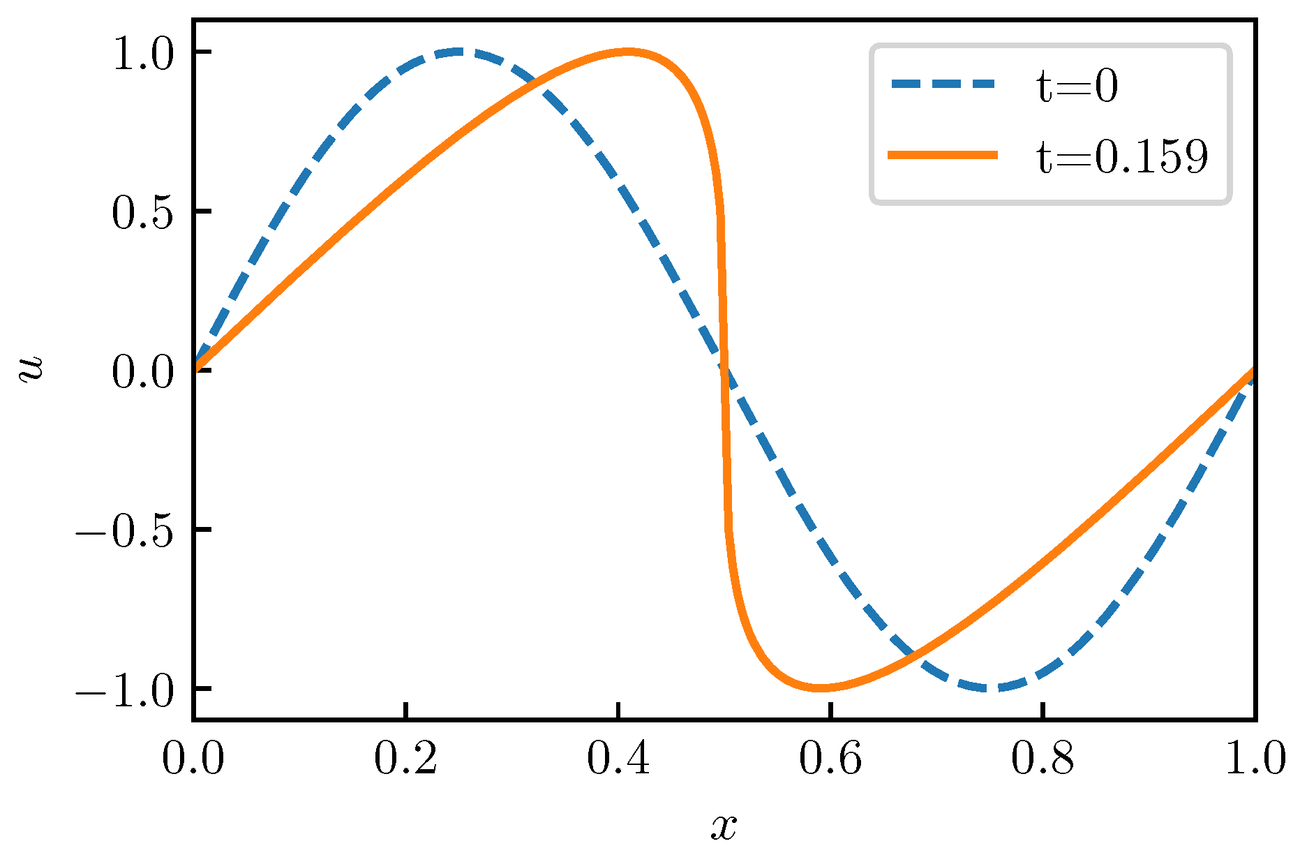
where n denotes the current timestep. The timestep corresponds to the CFL number . The end time is . The initial and final distributions of velocity are plotted in Figure A1. The velocity distribution at , which is predicted by Equation (A4), has a sharp variation at the center. The performance of the numerical scheme is measured by the accumulated error at the final timestep in this dynamic test.
Figure A1.
The distribution of u at and for the initial value problem of the 1-D Burgers equation.

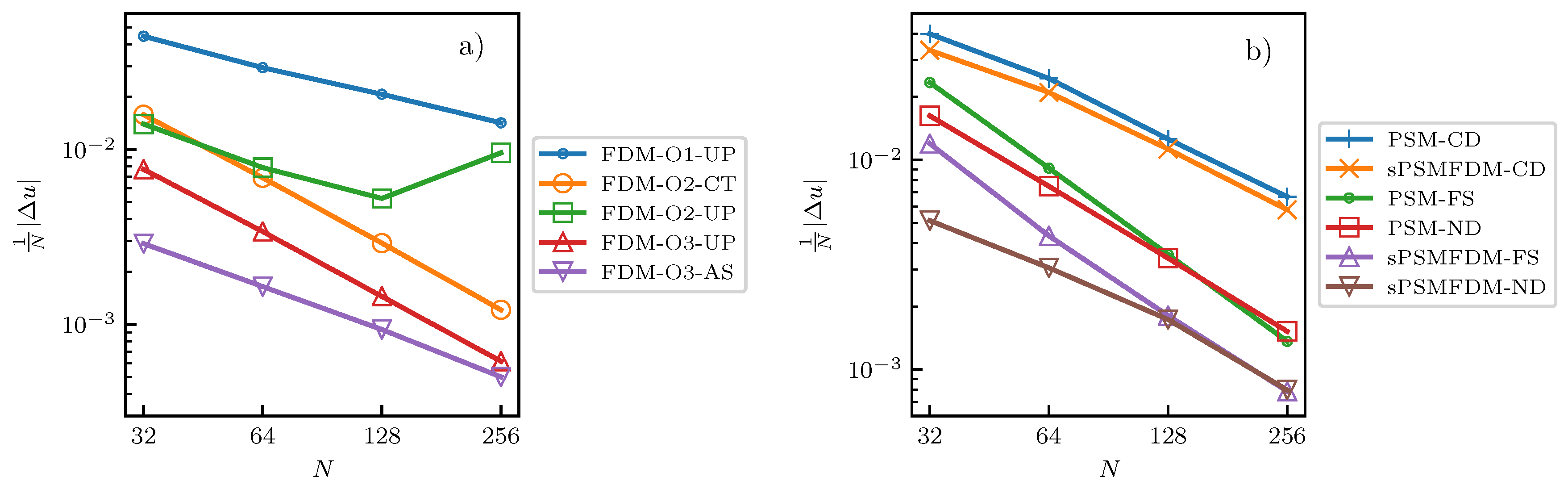
Several schemes for the finite-difference method (FDM) are tested to find the best option. The order of accuracy is up to the third. The stencil selection includes central difference scheme, upwind scheme, and an adaptive stencil scheme proposed by Hoar [53]. The results are shown in Figure A2a. The third order adaptive stencil scheme (FDM-O3-AS) produces the least error among the FDM schemes tested. Therefore FDM-O3-AS is used in the correction step of the hybrid approach sPSMFDM.
The width of the discontinuous region being smoothed is an important factor affecting the numerical error. In this test, we use a fixed ratio strategy, which determines the smoothing region by expanding the peak-to-trough region with a fixed ratio for each spatial resolution. An optimal ratio is found by iterative attempts to acquire the least error at each resolution. The optimal ratios are 1.67, 0.92, 0.51, and 0.24 for grid number 32, 64, 128, and 256, respectively. The trend of the optimal ratio shows that a narrower smoothing region is needed for a spatial discretization of more grid points.
Several schemes for the PSM are tested to show the effect of sPSMFDM and Fourier smoothing. The hybrid approach of pseudo-spectral method and finite-difference method (sPSMFDM) is generally more accurate than the classical spectral method (marked with PSM), as shown in Figure A2b. The schemes using Fourier smoothing-based dealiasing (marked with FS) are generally more accurate than the classical rule-based dealiasing (marked with CD).
Figure A2.
The dependence of the averaged error on the grid number in (a) FDM schemes and (b) spectral schemes. The finite-difference schemes are compared in (a), where FDM means the finite-difference method, O followed by a number means the order of accuracy, UP means upwind scheme, CT means central difference, and AS means adaptive stencil scheme. The spectral schemes are compared in (b), where PSM means pseudo-spectral method, sPSMFDM means the hybrid approach of smoothed PSM and FDM, CD means classical dealiasing, FS means Fourier smoothing, and ND means no dealiasing is applied.

References
- Wind Vision: A New Era for Wind Power in the United States; Technical Report; U.S. Department of Energy: Washington, DC, USA, 2015. Available online: https://www.energy.gov/eere/wind/wind-vision (accessed on 15 December 2018).
- Schlichting, H.; Gersten, K. Boundary-Layer Theory; Springer: Berlin, Germany, 2016. [Google Scholar]
- Hama, F.R.; Peterson, L.F. Axisymmetric Laminar Wake behind a Slender Body of Revolution. J. Fluid Mech. 1976, 76, 1–16. [Google Scholar] [CrossRef]
- Froude, R.E. On the Part Played in Propulsion by Differences of Fluid Pressure. Trans. Inst. Naval Arch. 1889, 30, 390–423. [Google Scholar]
- Sørensen, J.N. General Momentum Theory for Horizontal Axis Wind Turbines; Springer: Cham, Switzerland, 2016; Volume 4. [Google Scholar]
- Medici, D.; Alfredsson, P. Measurements on a Wind Turbine Wake: 3D Effects and Bluff Body Vortex Shedding. Wind Energy 2006, 9, 219–236. [Google Scholar] [CrossRef]
- Wu, Y.T.; Porté-Agel, F. Atmospheric Turbulence Effects on Wind-Turbine Wakes: An LES Study. Energies 2012, 5, 5340–5362. [Google Scholar] [CrossRef]
- Larsen, G.C. A Simple Wake Calculation Procedure; Number 2760 in Risø-M; Risø National Laboratory for Sustainable Energy, Technical University of Denmark: Lyngby, Denmark, 1988. [Google Scholar]
- Widnall, S.E. The Stability of a Helical Vortex Filament. J. Fluid Mech. 1972, 54, 641–663. [Google Scholar] [CrossRef]
- Felli, M.; Camussi, R.; Di Felice, F. Mechanisms of Evolution of the Propeller Wake in the Transition and Far Fields. J. Fluid Mech. 2011, 682, 5–53. [Google Scholar] [CrossRef]
- Sherry, M.; Nemes, A.; Lo Jacono, D.; Blackburn, H.M.; Sheridan, J. The Interaction of Helical Tip and Root Vortices in a Wind Turbine Wake. Phys. Fluids 2013, 25, 117102. [Google Scholar] [CrossRef]
- Howard, K.B.; Singh, A.; Sotiropoulos, F.; Guala, M. On the Statistics of Wind Turbine Wake Meandering: An Experimental Investigation. Phys. Fluids 2015, 27, 075103. [Google Scholar] [CrossRef]
- Foti, D.; Yang, X.; Sotiropoulos, F. Similarity of Wake Meandering for Different Wind Turbine Designs for Different Scales. J. Fluid Mech. 2018, 842, 5–25. [Google Scholar] [CrossRef]
- Sørensen, J.N.; Shen, W.Z. Numerical Modeling of Wind Turbine Wakes. J. Fluid Mech. 2002, 124, 393–399. [Google Scholar] [CrossRef]
- Calaf, M.; Meneveau, C.; Meyers, J. Large Eddy Simulation Study of Fully Developed Wind-Turbine Array Boundary Layers. Phys. Fluids 2010, 22, 015110. [Google Scholar] [CrossRef]
- Wu, Y.T.; Porté-Agel, F. Large-Eddy Simulation of Wind-Turbine Wakes: Evaluation of Turbine Parametrisations. Bound.-Layer Meteorol. 2011, 138, 345–366. [Google Scholar] [CrossRef]
- Porté-Agel, F.; Wu, Y.T.; Lu, H.; Conzemius, R.J. Large-Eddy Simulation of Atmospheric Boundary Layer Flow through Wind Turbines and Wind Farms. J. Wind Eng. Ind. Aerodyn. 2011, 99, 154–168. [Google Scholar] [CrossRef]
- Yang, D.; Meneveau, C.; Shen, L. Large-Eddy Simulation of Offshore Wind Farm. Phys. Fluids 2014, 26, 025101. [Google Scholar] [CrossRef]
- Kang, S.; Yang, X.; Sotiropoulos, F. On the Onset of Wake Meandering for an Axial Flow Turbine in a Turbulent Open Channel Flow. J. Fluid Mech. 2014, 744, 376–403. [Google Scholar] [CrossRef]
- Yang, X.; Sotiropoulos, F.; Conzemius, R.J.; Wachtler, J.N.; Strong, M.B. Large-Eddy Simulation of Turbulent Flow Past Wind Turbines/Farms: The Virtual Wind Simulator (VWiS). Wind Energy 2015, 18, 2025–2045. [Google Scholar] [CrossRef]
- Yang, D.; Meneveau, C.; Shen, L. Effect of Downwind Swells on Offshore Wind Energy Harvesting—A Large-Eddy Simulation Study. Renew. Energy 2014, 70, 11–23. [Google Scholar] [CrossRef]
- Sørensen, J.N.; Mikkelsen, R.F.; Henningson, D.S.; Ivanell, S.; Sarmast, S.; Andersen, S.J. Simulation of Wind Turbine Wakes Using the Actuator Line Technique. Philos. Trans. R. Soc. A 2015, 373, 20140071. [Google Scholar] [CrossRef]
- Wu, Y.T.; Porté-Agel, F. Modeling Turbine Wakes and Power Losses within a Wind Farm Using LES: An Application to the Horns Rev Offshore Wind Farm. Renew. Energy 2015, 75, 945–955. [Google Scholar] [CrossRef]
- Jonkman, J.M.; Annoni, J.; Hayman, G.; Jonkman, B.; Purkayastha, A. Development of FAST. Farm: A New Multi-Physics Engineering Tool for Wind-Farm Design and Analysis. In Proceedings of the 35th Wind Energy Symposium, Grapevine, TX, USA, 9–13 January 2017; p. 0454. [Google Scholar]
- Stevens, R.J.A.M.; Meneveau, C. Flow Structure and Turbulence in Wind Farms. Annu. Rev. Fluid Mech. 2017, 49, 311–339. [Google Scholar] [CrossRef]
- Stevens, R.J.; Martínez-Tossas, L.A.; Meneveau, C. Comparison of Wind Farm Large Eddy Simulations Using Actuator Disk and Actuator Line Models with Wind Tunnel Experiments. Renew. Energy 2018, 116, 470–478. [Google Scholar] [CrossRef]
- Bastankhah, M.; Porté-Agel, F. A New Analytical Model for Wind-Turbine Wakes. Renew. Energy 2014, 70, 116–123. [Google Scholar] [CrossRef]
- Jensen, N. A Note on Wind Generator Interaction; Number 2411 in Risø-M; Risø National Laboratory for Sustainable Energy, Technical University of Denmark: Lyngby, Denmark, 1983. [Google Scholar]
- Frandsen, S.; Barthelmie, R.; Pryor, S.; Rathmann, O.; Larsen, S.; Højstrup, J.; Thøgersen, M. Analytical Modelling of Wind Speed Deficit in Large Offshore Wind Farms. Wind Energy 2006, 9, 39–53. [Google Scholar] [CrossRef]
- Xie, S.; Archer, C. Self-Similarity and Turbulence Characteristics of Wind Turbine Wakes via Large-Eddy Simulation. Wind Energy 2015, 18, 1815–1838. [Google Scholar] [CrossRef]
- Foti, D.; Yang, X.; Guala, M.; Sotiropoulos, F. Wake Meandering Statistics of a Model Wind Turbine: Insights Gained by Large Eddy Simulations. Phys. Rev. Fluids 2016, 1, 044407. [Google Scholar] [CrossRef]
- Germano, M.; Piomelli, U.; Moin, P.; Cabot, W.H. A Dynamic Subgrid-Scale Eddy Viscosity Model. Phys. Fluids A Fluid Dyn. 1991, 3, 1760–1765. [Google Scholar] [CrossRef]
- Kim, J.; Moin, P. Application of a Fractional-Step Method to Incompressible Navier-Stokes Equations. J. Comput. Phys. 1985, 59, 308–323. [Google Scholar] [CrossRef]
- Moeng, C.H. A Large-Eddy-Simulation Model for the Study of Planetary Boundary-Layer Turbulence. J. Atmos. Sci. 1984, 41, 2052–2062. [Google Scholar] [CrossRef]
- Albertson, J.D.; Parlange, M.B. Surface Length Scales and Shear Stress: Implications for Land-Atmosphere Interaction over Complex Terrain. Water Resour. Res. 1999, 35, 2121–2132. [Google Scholar] [CrossRef]
- Yang, X.; Zhang, X.; Li, Z.; He, G.W. A Smoothing Technique for Discrete Delta Functions with Application to Immersed Boundary Method in Moving Boundary Simulations. J. Comput. Phys. 2009, 228, 7821–7836. [Google Scholar] [CrossRef]
- Martínez-Tossas, L.A.; Churchfield, M.J.; Meneveau, C. Optimal Smoothing Length Scale for Actuator Line Models of Wind Turbine Blades Based on Gaussian Body Force Distribution. Wind Energy 2017, 20, 1083–1096. [Google Scholar] [CrossRef]
- Yang, X.; Sotiropoulos, F. A New Class of Actuator Surface Models for Wind Turbines. Wind Energy 2018, 21, 285–302. [Google Scholar] [CrossRef]
- Li, Q.; Bou-Zeid, E.; Anderson, W. The Impact and Treatment of the Gibbs Phenomenon in Immersed Boundary Method Simulations of Momentum and Scalar Transport. J. Comput. Phys. 2016, 310, 237–251. [Google Scholar] [CrossRef]
- Hou, T.Y.; Li, R. Computing Nearly Singular Solutions Using Pseudo-Spectral Methods. J. Comput. Phys. 2007, 226, 379–397. [Google Scholar] [CrossRef]
- Yang, D.; Shen, L. Simulation of Viscous Flows with Undulatory Boundaries. Part I: Basic Solver. J. Comput. Phys. 2011, 230, 5488–5509. [Google Scholar] [CrossRef]
- Shen, L.; Zhang, X.; Yue, D.K.P.; Triantafyllou, M.S. Turbulent Flow over a Flexible Wall Undergoing a Streamwise Travelling Wave Motion. J. Fluid Mech. 2003, 484, 197–221. [Google Scholar] [CrossRef]
- Sotiropoulos, F.; Angelidis, D.; Calderer, A.; Ge, L.; Gilmanov, A.; Kang, S.; Khosronejad, A.; Le, T.; Yang, X. VFS-Wind, Virtual Flow Simulator. Available online: http://safl-cfd-lab.github.io/VFS-Wind/ (accessed on 20 September 2016).
- Chamorro, L.P.; Porté-Agel, F. Effects of Thermal Stability and Incoming Boundary-Layer Flow Characteristics on Wind-Turbine Wakes: A Wind-Tunnel Study. Bound.-Layer Meteorol. 2010, 136, 515–533. [Google Scholar] [CrossRef]
- Yang, X.; Sotiropoulos, F. On the Predictive Capabilities of LES-Actuator Disk Model in Simulating Turbulence Past Wind Turbines and Farms. In Proceedings of the 2013 American Control Conference, Washington, DC, USA, 17–19 June 2013; pp. 2878–2883. [Google Scholar]
- Tseng, Y.H.; Meneveau, C.; Parlange, M.B. Modeling Flow around Bluff Bodies and Predicting Urban Dispersion Using Large Eddy Simulation. Environ. Sci. Technol. 2006, 40, 2653–2662. [Google Scholar] [CrossRef]
- Sunada, S.; Sakaguchi, A.; Kawachi, K. Airfoil Section Characteristics at a Low Reynolds Number. J. Fluids Eng. 1997, 119, 129–135. [Google Scholar] [CrossRef]
- Jiang, H.B.; Li, Y.R.; Cheng, Z.Q. Relations of Lift and Drag Coefficients of Flow around Flat Plate. Appl. Mech. Mater. 2014, 518, 161–164. [Google Scholar] [CrossRef]
- Chamorro, L.P.; Porté-Agel, F. A Wind-Tunnel Investigation of Wind-Turbine Wakes: Boundary-Layer Turbulence Effects. Bound.-Layer Meteorol. 2009, 132, 129–149. [Google Scholar] [CrossRef]
- Johansson, P.B.V.; George, W.K. The Far Downstream Evolution of the High-Reynolds-Number Axisymmetric Wake behind a Disk. Part 1. Single-Point Statistics. J. Fluid Mech. 2006, 555, 363–385. [Google Scholar] [CrossRef]
- Uberoi, M.S.; Freymuth, P. Turbulent Energy Balance and Spectra of the Axisymmetric Wake. Phys. Fluids 1970, 13, 2205–2210. [Google Scholar] [CrossRef]
- Hu, H.; Yang, Z.; Sarkar, P. Dynamic Wind Loads and Wake Characteristics of a Wind Turbine Model in an Atmospheric Boundary Layer Wind. Exp. Fluids 2012, 52, 1277–1294. [Google Scholar] [CrossRef]
- Hoar, R.H.; Vogel, C.R. An Adaptive Stencil Finite Difference Method for First Order Linear Hyperbolic Systems. Ph.D. Thesis, Montana State University-Bozeman, College of Letters & Science, Bozeman, MT, USA, 1995. [Google Scholar]
Figure 1.
The estimation of aerodynamic lift force and drag force on an airfoil section. The upstream fluid velocity is decomposed into a parallel component and a perpendicular component with respect to the rotation axis. The rotation speed is the product of the angular velocity and the distance r to rotation center. is the relative velocity in coordinate system of the airfoil section.

Figure 2.
Illustration of the hybrid approach sPSMFDM. The velocity field at for an initial value problem of 1D Burgers equation is shown in (a). The original velocity field is denoted by —, the smoothed field is denoted by △, and the points for cubic interpolation are denoted by □. The spatial derivative is plotted in (b). The analytic solution is denoted by —, the result of the hybrid approach sPSMFDM is denoted by +. The result of PSM on a smoothed input (sPSM) is denoted by △. The result of FDM for correction of sPSM is denoted by ∘. The result of PSM on the original velocity field is denoted by × for comparison.

Figure 3.
Illustration of the computational domain. The wind blows in the x direction. A turbine model is deployed at a distance of 0.75 m from the inlet. A turbulent inflow database is imported in the velocity relaxation zone upstream.
Figure 3.
Illustration of the computational domain. The wind blows in the x direction. A turbine model is deployed at a distance of 0.75 m from the inlet. A turbulent inflow database is imported in the velocity relaxation zone upstream.

Figure 4.
Turbine parameterizations for rotor GWS/EP-6030×3.

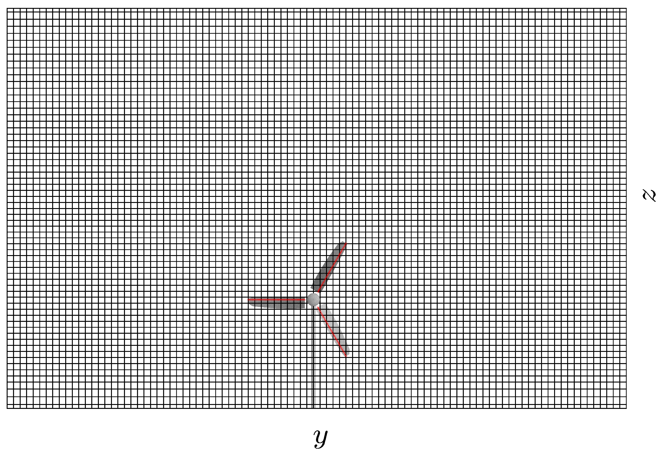
Figure 5.
The grid discretization for fluid and turbine in plane. The rectangular cells are for fluids. The red lines inside the turbine geometry are actuator line elements.
Figure 5.
The grid discretization for fluid and turbine in plane. The rectangular cells are for fluids. The red lines inside the turbine geometry are actuator line elements.

Figure 6.
Comparison of the contours for , the streamwise advection of turbulent kinetic energy (TKE), calculated by (a) the standard pseudo-spectralmethod and (b) the proposed sPSMFDM, respectively.
Figure 6.
Comparison of the contours for , the streamwise advection of turbulent kinetic energy (TKE), calculated by (a) the standard pseudo-spectralmethod and (b) the proposed sPSMFDM, respectively.

Figure 7.
Vertical profiles of time-averaged velocity , turbulence intensity , and time-averaged Reynolds stress at two different distances downstream of the turbine: subplots (a–c) are at and subplots (d–f) are at . The results from our LES are denoted by —; the measurement data in wind-tunnel experiment of [44] are denoted by ∘. In (a,d), the inflow profiles are plotted for reference: the LES results of inflow are denoted by ; the wind-tunnel data of upstream flow are denoted by △. The heights of rotor top, rotor center, and rotor bottom are denoted by ⋯.

Figure 8.
The mean velocity of the turbine wake flow. The bold line in (a) represents the rotation region of turbine blades. The velocity along the dashed line in (a) is plotted in (b).
Figure 8.
The mean velocity of the turbine wake flow. The bold line in (a) represents the rotation region of turbine blades. The velocity along the dashed line in (a) is plotted in (b).

Figure 9.
The self-similarity of the mean velocity deficit. The characteristic scales of velocity deficit and wake width are shown in (a,b), respectively, where the dotted lines are the boundaries of the three stages of wake development. The normalized spanwise profile of mean velocity deficit at the stages II and III are plotted with circular points in (c) and the dashed line is a Gaussian distribution fitting for the normalized profile.

Figure 10.
The normalization for the spanwise profile of the Reynolds stress component . In (a), the spanwise profiles are normalized by a fixed scale for all downstream distances. In (b), the definitions of the characteristic scales in are annotated. In (c), the spanwise profiles in are normalized by the characteristic scales. In the normalization, is subtracted, which is the average of for grid points between the two positive peaks.

Figure 11.
The streamwise development of the characteristic scales of the Reynolds stress component . The spanwise averaging is shown in (a). The characteristic Reynolds stress is shown in (b). In (a,b), the Reynolds stress is normalized by the characteristic velocity deficit . The characteristic width is shown in (c). The dotted lines denote the boundary of the stage II and III of the wake development.

Figure 12.
The normalization for the spanwise profile of the Reynolds stress component . In (a), the spanwise profiles are normalized by a fixed scale for all downstream distances. In (b), the definitions of the characteristic scales in are annotated. In (c), the spanwise profiles in are normalized by the characteristic scales. The vertical coordinate in (c) is defined by Equation (20). The dashed line in (c) is the theoretical solution Equation (19) for the normalized profile of . The dotted lines in (c) are the boundaries of the inner and the outer regions for the spanwise distribution.

Figure 13.
The streamwise development of the characteristic scales of the Reynolds stress component . The characteristic widths of the inner region and outer region are shown in (a,b), respectively, where the dotted line is the boundary of the stage II and III of the wake development. In (c), the characteristic Reynolds stress is normalized by the characteristic velocity deficit .

Figure 14.
The comparison of the characteristic scales. Four velocity-like scales are shown in (a), three of which are shown in (b) as an enlarged view. The length scales are shown in (c). The scales for the mean velocity deficit , Reynolds stress components , and are denoted by —, +, and ∘, respectively. The square root of the spanwise mean of the Reynolds stress is denoted by –.

Figure 15.
Budgets of the mean momentum Equation (22) along (a) radial direction and (b) streamwise direction.
Figure 15.
Budgets of the mean momentum Equation (22) along (a) radial direction and (b) streamwise direction.

Figure 16.
Wake meandering. The instantaneous centerline of the meandering velocity deficit is shown in (a). The superposition of centerlines is shown in (b). The dotted and dashed lines in (b) are the edges extracted from the superposition of centerlines at all timesteps, while the circles are the wakeline at 25 random timesteps. The dashed lines A and B in (b) are the locations where the centerline may collide with the tip vortices.

Figure 17.
The averaged vertical vorticity in the horizontal plane at the hub height. The positive and negative peaks of the vorticity are marked with the dashed lines.
Figure 17.
The averaged vertical vorticity in the horizontal plane at the hub height. The positive and negative peaks of the vorticity are marked with the dashed lines.

Figure 18.
The averaged TKE in the horizontal plane at the hub height.

© 2019 by the authors. Licensee MDPI, Basel, Switzerland. This article is an open access article distributed under the terms and conditions of the Creative Commons Attribution (CC BY) license (http://creativecommons.org/licenses/by/4.0/).
Share and Cite
MDPI and ACS Style
Lyu, P.; Chen, W.-L.; Li, H.; Shen, L. A Numerical Study on the Development of Self-Similarity in a Wind Turbine Wake Using an Improved Pseudo-Spectral Large-Eddy Simulation Solver. Energies 2019, 12, 643. https://doi.org/10.3390/en12040643
AMA Style
Lyu P, Chen W-L, Li H, Shen L. A Numerical Study on the Development of Self-Similarity in a Wind Turbine Wake Using an Improved Pseudo-Spectral Large-Eddy Simulation Solver. Energies. 2019; 12(4):643. https://doi.org/10.3390/en12040643
Chicago/Turabian StyleLyu, Pin, Wen-Li Chen, Hui Li, and Lian Shen. 2019. "A Numerical Study on the Development of Self-Similarity in a Wind Turbine Wake Using an Improved Pseudo-Spectral Large-Eddy Simulation Solver" Energies 12, no. 4: 643. https://doi.org/10.3390/en12040643
Note that from the first issue of 2016, this journal uses article numbers instead of page numbers. See further details here.