The Effects of Electrification on School Enrollment in Bangladesh: Short- and Long-Run Perspectives

Abstract

This paper aims to show the impact of access to electricity on school enrollment in Bangladesh. It offers an empirical investigation of the relationship between access to electricity and school enrollment statuses, such as grade progression, repetition, and non-attendance. The data were taken from Bangladesh’s Multiple Indicator Cluster Survey (MICS) database 2012–2013 provided by the Bangladesh Bureau of Statistics (BBS) and UNICEF; the data include two years of grading information for children of ages ranging from 5–15. We applied the propensity score matching (PSM) and the Markov schooling transition model using matched sample data. The results show that access to electricity has a significant positive effect on grade progression and a significant negative effect on non-attendance in the short run as well as in the long run. The simulation result shows that the non-attendance rate is lower and the school enrollment rate for children grades 9-11 is higher in the electrified areas compared to unelectrified areas. This result suggests that access to electricity is an important strategic indicator for increasing school enrollment in both primary and secondary schools.

1. Introduction

Light is a basic human need, and is also considered an important indicator of everyday lifestyle. Changes in lighting also change people’s performance. Several mechanisms contribute to increasing human performance through improved lighting, such as visual performance, visual comfort, interpersonal skills, problem-solving, and change processes [1]. Lighting also has non-visual effects. Good quality lighting affects performance, mood, attention, and synchronization [2]. Most households in unelectrified regions use kerosene lamps, candles, and solar lanterns as sources of indoor lighting. These types of lighting adversely affect the safety, health, and environment of household members. We consider access to electricity to be access to lighting sources. This study extends reflection on the link between access to electricity and school enrollment. It is motivated by an empirical study based in rural Mexico that shows that a school subsidy program is associated with higher enrollment rates, less grade repetition, better grade progression, and lower dropout rates [3]. However, limited studies conducted in several developing countries show the effects of access to electricity on children’s education in terms of study time and school attainment. We want to examine the effects of electrification on school enrollment (grade progression, repetition, and non-attendance) in the short run as well as the long run.

Several assessments have been undertaken of the impacts of electricity on socio-economic development. Access to electricity reduces the time spent by children on activities such as gathering fuelwood and fetching water, promotes the home study and enables the use of educational media and communications in school [4]. A study by the United Nations Development Programme (UNDP)/World Health Organization (WHO) showed that education enrollment ratios correlate with access to electricity [5]. One macro level study using panel data showed that long-run bidirectional causality exists between electricity consumption and five human development indicators: per capita gross domestic product (GDP), consumption expenditure, urbanization rate, life expectancy at birth, and adult literacy rate [6]. Many researchers have shown that a positive relationship exists between access to modern energy and economic development. Affordable and accessible modern energy plays an essential role in the development and ensures sustainable development [7,8,9]. However, electricity and income exhibit two-way causality: income explains the potential to connect to electricity, and connection to electricity has a substantial and significant effect on income [10]. Empirical studies based on electrification have generally supported the benefits to health, education, and income; however, these claims are weak [11,12]. Home electrification helps to improve children’s education [13]. One study claimed that interactions between energy and development are complex and not causal [14]. The impact of electrification appears to increase the hours of work for men and women, in particular, increasing women’s employment by releasing them from home production [15]. Dinkelman [15] applied two identification strategies, namely, instrumental variables and fixed-effect approaches, to overcome the endogeneity problem of electrification. The confounding trend of electrification makes it more difficult to identify the treatment effect on the economy. We assume that no confounder is present in our model, and we apply propensity score matching (PSM) to identify the impact of electrification on school enrollment.

Household access to electricity has a significant positive impact on children’s nutritional status as a result of increased wealth. Children’s nutritional outcomes are affected by causal channels such as wealth, fertility, and television [16]. One empirical study estimated the causal impact and showed that electrification has a significantly positive impact on household income, expenditure, and school enrollment in Bangladesh [17]. Another study based on county-level data from urban and rural Brazil showed that electrification has a substantial positive and significant effect on income, literacy, and the enrollment rate components of education [18]. Furthermore, a study indicates that electricity from a solar home system increases the study time of children in Bangladesh [19]. The electrification of homes, schools, and communities has a significant effect on educational outcomes [20]; moreover, electrification has a positive effect on female enrollment in school and on reading capability for both boys and girls [21].

Bangladesh was the first country in the world to implement school incentive programs to increase school attendance, especially for children from low-income families. These incentives include free tuition, books, food provided in exchange for school attendance (Food for Education), and a stipend for female students. Over the past two decades, a significant proportion of education policies has been applied towards increasing school enrollment through Food for Education and stipends for poor students and female students. This type of education policy suggests that income is the primary barrier to children continuing their studies in school. The cash incentive program has a direct effect on school enrollment, and low-income families respond positively by sending their children to school. Evidence from descriptive statistics shows that school incentive programs (Food for Education and female student stipends) in Bangladesh increase children’s school attendance, and decrease the out-of-school rate and child labor activity [22]. Another study, based on descriptive statistics and a multivariate model, also showed that the Food for Education program increased school enrollment, promoting school attendance and preventing dropping out [23]. The motivation for the current study is to assess the impact of electrification on school enrollment. In Bangladesh, providing continuous electricity is a major problem, and load shedding is a common scenario in rural areas. Access to electricity has an indirect effect on children’s study due to the quality of light. In our study, we want to examine the impact of access to electricity on school enrollment.

Education is an essential tool to strengthen human resources and maintain steady development in any country. In Bangladesh, gross enrollment has approached the universal level, and the primary school completion rate has remained at 60% since 2000 [24]. Grade repetition, non-attendance, and dropping out also remain major problems. Some research has shown that dropping out occurs due to either financial problems or a lack of interest in education. Several factors potentially drive these causes such as age, gender, poor physical condition, geographical location, household characteristics, and economic hardship [25,26]. Study completion also relates to gender, family income, and the cost of school fees, books, uniforms, and transportation [27].

Several pathways can be followed to identify the possible causal impacts of electrification on school enrollment. First, the use of electricity enhances the income opportunities of the household through extended work hours, and a greater income prompts parents to send their children to school to achieve a better future based on the social and financial returns of education. Second, electricity can improve the lighting status of the household and replace traditional candles and kerosene lamps. Household electrification leads to a reduction in indoor air pollution [28]. This helps children to study longer and with better concentration. It also allows parents to take better care of their children by allowing more flexible use of time. Third, access to electricity also provides families with more, better quality information through information technology such as cell phones and television. We can speculate that the benefits from access to electricity can be explained by these three causal channels, but we are unable to estimate the above causal impacts due to the absence of data.

Most previous studies use different ways to show the impact of access to electricity on education. This type of nexus states the positive benefit of electricity use on education without explaining the causal relationship. Some studies report correlations that appear to show the positive impact of electricity use, although multiple socio-economic factors might impact on education. The existing literature also fails to capture the reverse causalities and the potential bias of access to electricity on educational outcomes. The potential drawbacks of studies in the existing literature are as follows: (1) most studies rely on correlations and (2) most studies adopt a single indicator, such as the enrollment rate, dropout rate, or grade repetition rate; thus, they cannot assess the long-term effects of electricity on school enrollment.

For the purpose of evaluation, we applied a propensity score matching (PSM) approach that captures different covariates for participation in a single propensity score. This study adopts a non-experimental strategy to assess the impact of electricity on school enrollment in Bangladesh. Thus, by using panel data from the Multiple Indicators Cluster Survey (MICS) database, through PSM, we can isolate the causal effect of access to electricity on school enrollment. We applied the nearest neighbor matching (NNM) method to estimate the impact of access to electricity, where each treatment unit was matched to the comparison unit with the closest propensity score. We constructed transition matrices for both groups based on age and took the difference to estimate the short- and long-run impact of access to electricity on school enrollment. The data analyzed in this study cover two years of information on the grades of children studying in primary and secondary schools. Thus, it is impossible to assess the long-run impact due to the short time span of the data. However, the long-run impact is our key interest as access to electricity is an important indicator of socio-economic development. Therefore, we propose a method for simulating the effects through age transition matrices. The results, based on our simulation, indicate that if children are at age 5 when they began attending school and continued to study up to age 15, their school enrollment distribution would change substantially. Moreover, non-attendance would decrease by 2.48%, and transition to grade 11 would increase by 0.43% in electrified regions compared to unelectrified regions. The simulation results also show that a substantial impact of electrification on school enrollment occurs for grades 9–11.

The rest of the paper is organized as follows: Section 2 provides the estimation methods, comprising the matching procedure and the Markov schooling transition model. Section 3 presents a description of the data. Section 4 provides the empirical results and discussion, while Section 5 presents the conclusions.

2. Estimation Methods

If access to electricity were randomly assigned to households, it would be an experiment. We could evaluate by household the causal effect of access to electricity on children’s school enrollment as the difference in average school enrollment between those with and those without access to electricity. However, home electrification is based on each head of the household’s self-selection instead of random assignment. The government electrification program is also influenced by political pressure, regional priority, and donors’ attitudes [29]. Rich households enjoy more opportunity to install electrification compared to poor households. We can say that the treatment assignment is not random and that a systematic difference exists between the with and the without electricity groups. Selection bias could possibly occur as unobservable factors influence both the treatment and outcome variables. Hence, if we apply the ordinary least squares (OLS) method, biased estimates would be the result. We cannot apply the difference-in-difference (DID) method as we have one-shot data. We can also control for selection bias by employing an instrumental variable (IV) approach. Finding the appropriate instrument from the data set is difficult [30].

Access to electricity could be considered a non-randomized treatment, with the treatment effect based solely on observable characteristics. The PSM estimator is a popular method among analysts, especially for social program evaluation. In our study, we want to construct a transition matrix that reveals the grade transition of children between the two groups; however, matched samples are needed to construct this kind of transition matrix. The PSM method assists our study in grasping matched samples. We then apply the Markov schooling transition model based on these matched samples. The short- and long-run impacts on school enrollment are thereby evaluated. However, the recent empirical literature has identified some bias in PSM [31] which is associated with several factors, including: the selection of the unobservable; the failure of the common support condition; the failure to control for local differences; and the selection of the dependent variable for both control and treatment groups [32].

2.1. Matching Procedure

We can estimate the average treatment effect (ATE) in a counterfactual framework, in accordance with Rosenbaum and Rubin [33], as follows:

$$ATE=Y_i^{AE}-Y_i^{NAE}$$

(1)

where $Y_i^{AE}$ and $Y_i^{NAE}$, respectively, denote school enrollment of children in a household that has access to electricity and children in a household that does not have access to electricity. As both $Y_i^{AE}$ and $Y_i^{NAE}$ are not normally distributed, we can express the normal distribution equation as follows:

$$Y_i=T_i{Y}_{iAE}+\left(1-T_i\right)Y_{iNAE} T=0, 1$$

(2)

If we consider P as the probability of observing a household with access to electricity, that is, $T=1$, the average treatment effect can be written as:

$$ATE=P·\left[E\left(Y_{AE}|T=1\right)-E\left(Y_{NAE}|T=1\right)\right]+\left(1-P\right)\left[E\left(Y_{AE}|T=0\right)-E\left(Y_{NAE}|T=0\right)\right]$$

(3)

Equation (3) indicates the effect of access to electricity on the entire samples. This is measured by the weighted average of the effect of access to electricity on the treated sample and the control sample with each weighted by its relative frequency. It is not possible to estimate the causal inference of the unobserved counterfactuals, ($E\left(Y_{AE}|T=0\right)$ and $E\left(Y_{NAE}|T=1\right)$) [32].

An important issue in evaluating the impact of access to electricity on children’s school enrollment is that we might not obtain counterfactual information from the existing data sets. We want to solve the problem by using the PSM method that enables the construction of a single propensity score from the pre-treatment characteristics [33]. We can then use the propensity score for matching with scores from similar individuals., Based on the treatment, the PSM method, given the conditional pre-treatment variables, is as follows:

$$p\left(X\right)=\mathrm{Pr}\left[T=1|X\right]=E\left[T|X\right]; p\left(X\right)=F\left\{h\left(X_i\right)\right\}$$

(4)

where $F\{.\}$ can be normal or probit cumulative distribution and X is a vector of covariate characteristics.

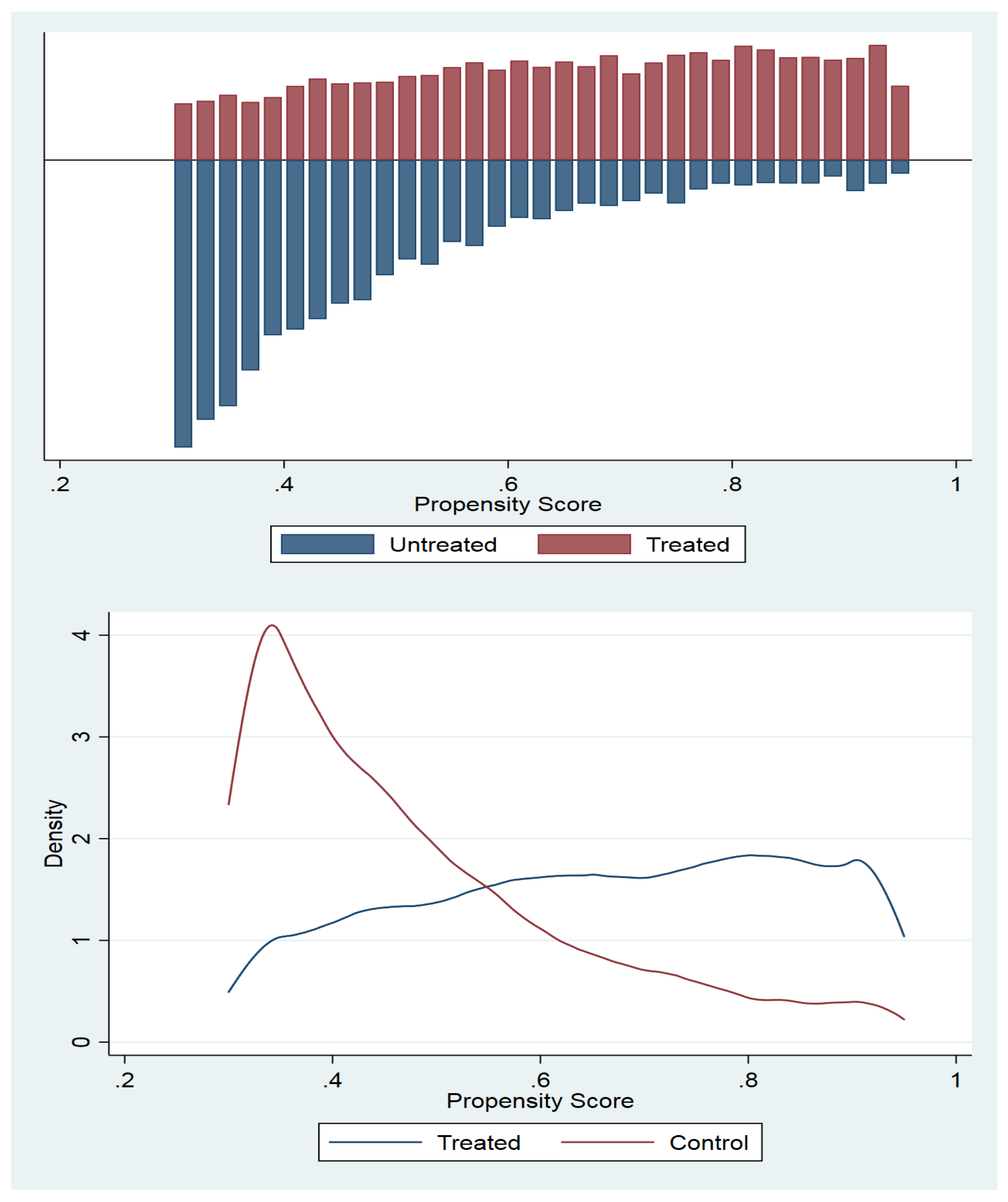
We need to fulfill two conditions, namely, the conditional independence assumption (CIA) and common support between the two groups. The matching method can be meaningfully applied over regions of common support (see Appendix A Figure A1). A strong argument is that a person with the same propensity score should have the same X values, with a positive probability of being both treated and control [34]. The average treatment effect for the treated (ATET), based on propensity scores, can be estimated as follows:

$$\begin{gathered} ATET=E\left\{Y_{iAE}-Y_{iNAE} |T=1\right\}, \\ ATET=E\left[E\left\{Y_{iAE}-Y_{iNAE} |T_i=1, p\left(X\right)\right\}\right], \\ ATET=E[E\left\{Y_{iAE}|T_i=1, p\left(X\right)\right\}-E\left\{\right(Y_{iNAE}|T_i=0, p\left(X\right)\left\}\right|T=1]. \end{gathered}$$

(5)

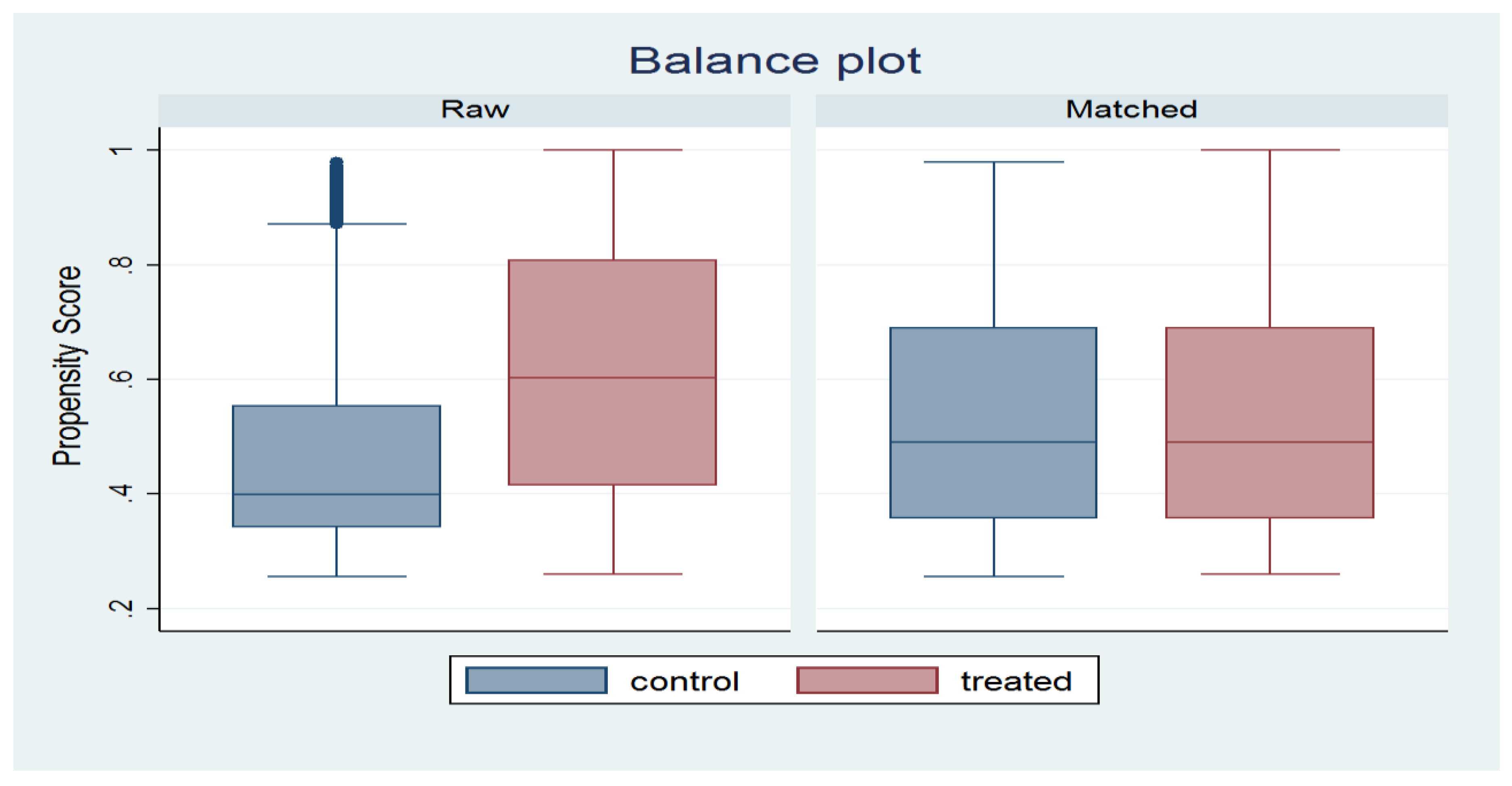
This indicates the average difference between those who are treated and their matching partners. A popular way to estimate the treatment effect is the nearest neighbor matching (NNM) method. We estimate the treatment effect based on the propensity score, but not on the condition of all covariates. The covariate balancing between the treatment and control groups after matching needs to be checked (see Appendix A Figure A2).

Justification of Covariate Selection

The determinants of household access to grid electricity comprise many factors, of which household income is considered to be the main factor. A study in South Africa showed that household income and electricity price are the main determinants of electricity demand [35]. Household size and dwelling type are also important determinants of electricity consumption [36]. For gaining access to electricity, household location is important. Access to electricity for a rural household has a more significant positive effect on education and health attainments than is the case for an urban household [37]. It is expected that electricity demand in rural areas is mainly for the purpose of lighting, with lighting also shown to affect children’s education in developing countries. Grid electrification is not possible in rural areas due to budget constraints. Kanagawa and Nakata [38] reported that access to electricity was linked to infrastructure, supply capacity, government policy, and international cooperation.

Adoption of electricity at the household level depends on various socio-economic characteristics of the household, its geographical position, government policy, etc. Identifying the determinants of access to electricity at the household level is at times difficult due to a mix of individual characteristics and geographical factors. Khandker et al. [17] showed that, in Bangladesh, the impact of access to grid electrification on income and educational outcome is positive and significant. In their study, they applied PSM and the instrumental variable (IV) approach to estimate the causal effect of access to electricity on income, expenditure, and educational outcome. Their set of covariates included: gender, age, and level of education of head of household; household landholding, dwelling, and drinking water, village price of kerosene, etc. to estimate the propensity score of household access to electricity.

In another study, Khandker et al. [39] showed that, in Vietnam, the impact of access to grid electrification had significant positive effects on a household’s cash income, expenditure, and educational outcomes. They applied difference-in-difference (DID), DID with fixed effect (FE) regression, and PSM-DID to estimate the causal effect of electrification. In their study, the propensity score of access to grid electricity was estimated based on: gender, age, and education level of head of household; household landholding and running water, commune price of kerosene, etc.

Kumar and Rauniyar [40] applied PSM to show the impact of access to electricity on income and educational outcomes in Bhutan. They found that access to electricity has a positive impact on non-farm income and educational outcomes. To estimate the propensity score, they used: household size; gender and age of head of household; amount of household land; access to tap water; house structure; religion; and distance as covariates.

In the current study, we chose age, gender, and education level of head of household; family size; number of sleeping rooms; location, having a water pump; and the wealth score from the MICS database as covariates. The data did not include any income or expenditure information, and the wealth score was used as a proxy of income variable.

2.2. Markov Model of Schooling Transition

We used the Markov schooling transition probability matrix to show the impact of access to electricity on school enrollment, measured by factors such as grade progression, grade repetition, and non-attendance. This transition matrix provides a convenient framework that can be used to assess the impact on various dimensions.

In Bangladesh, three possible schooling states are available for 5- or 6-year-old children: non-attendance, enrolled in grade 1, or enrolled in grade 2. In Bangladesh, most 6-year-old children are enrolled in grade 1. For 7-year-old children, four possible schooling states exist: enrolled in grade 3, enrolled in grade 2, enrolled in grade 1, and non-attendance. The most common state for 7-year-old children is enrolled in grade 2.

A transition probability matrix describes the transition using various ages for children by their schooling state. We can obtain the distribution of 7-year-old children’s schooling state given the initial distribution of 6-year-olds in the following way:

$${\left(\begin{array}{c}{f}_3^7\\ f_2^7\\ f_1^7\\ f_{NA}^7\end{array}\right)}_{4\times 1}= {\left(\begin{array}{ccc}{A}_{11}^6& A_{12}^6& A_{13}^6\\ A_{21}^6& A_{22}^6& A_{32}^6\\ A_{31}^6& A_{32}^6& A_{33}^6\\ A_{41}^6& A_{42}^6& A_{43}^6\end{array}\right)}_{4\times 3}{\left(\begin{array}{c}{f}_2^6\\ f_1^6\\ f_{NA}^6\end{array}\right)}_{3\times 1}$$

The above matrix can be written in the following equation:

$$f^7=A^6{f}^6$$

(6)

where $A^6$ is the transition matrix for children aged 6 years old, and $f^6$ is the vector of schooling state proportions. We need to increase the number of rows in the A matrix with age as the number of potential grade levels increases.

2.3. Estimating Short-Run Impacts: 1-Year Impacts

In our study, we had grading information for more than 30,000 children from electrified regions and more than 26,000 children from unelectrified regions. The nearest neighbor matching (NNM)-based PSM matched the data between the two types of region. We obtained grade information for 26,499 children for both the treatment and control groups. We considered that the 1-year impact of access to electricity for children of a given age a could be evaluated by comparing the age-specific transition matrix estimated for the treated (unelectrified) and control (electrified) groups:

$${\hat{A}}_{T=1}^a-{\hat{A}}_{T=0}^a$$

We construct transition matrices for both groups; comparing the short-run effects of access to electricity on grade progression, repetition, and non-attendance at each age; and take the difference to estimate the impact of access to electricity. Matching ensures that the effect of access to electricity can be calculated by simply taking the difference between the two groups.

We also test whether the observed treatment and control group differences are statistically significant based on Pearson’s chi-squared tests. We examine two types of tests: an equivalence test between the treatment and control transition matrices, and a test of equivalence between the individual columns of the matrices.

2.4. Simulating Long-Run Impact of Access to Electricity

The long-run impact of access to electricity on school enrollment is of greater interest to us for policy purposes. We observed children in our data set for only two years, so we cannot directly estimate the long-run impact of access to electricity. Therefore, we apply a simulation approach that uses the Markov schooling transition model to predict the effects of access to electricity on school enrollment at age 15. We make two assumptions about the greater validity of our evaluation process as follows:

Assumption 1:

The number of children at age four is the same as the number expected to go to school at age five.

Assumption 2:

The age-specific transition matrices are consistent over time.

Under both assumptions and given an initial vector of the state proportion at each age, the predicted schooling state can be found by the product of the previous age enrollment status and the state proportions of the current age. The mathematical expression for the predicted school enrollment status of 6-year-old children for both treatment and control groups is as follows:

$${\tilde{f}}_g^6={\widehat{f}}_g^5 {\widehat{A}}^6$$

where we indicate the predicted enrollment status with a tilde $(~)$ and things that are directly estimated from the age transition matrices with a hat $(^)$. More generally, the predicted grade status at any age a is given by:

$${\widehat{f}}_g^a={\widehat{f}}_g^{a-1} {\widehat{A}}^a$$

We started at age 5 and completed the transition at age 15. At the end of the transition at age 15, we obtained various grade levels and non-attendance information for both treatment and control groups and then took the difference to judge the long-run impacts of access to electricity.

3. Description of the Data

The data are from Bangladesh’s MICS database 2012–2013 created by the Bangladesh Bureau of Statistics (BBS), the Ministry of Planning, Bangladesh, and the United Nations Children’s Fund (UNICEF). The survey collected comprehensive, detailed information on a wide range of topics, including: household information; household characteristics; education; water and sanitation; children under five; women; salt iodization; and water quality testing. The data provide estimates at the national level with disaggregated data by division, location, gender, age, education level, and wealth quintiles. Bangladesh’s MICS database 2012–2013 is based on a sample of 51,895 interviewed households, and it offers a comprehensive picture of children’s education and nutrition. The data were panel data for two years that captured information about children’s school attendance and grades. From the data set, most 5- and 6-year-olds are enrolled in grade 1 or one of the three possible schooling states as follows:

(1)

Non-attendance

(2)

Enrolled in grade 1 or

(3)

Enrolled in grade 2.

For children who are 7 years old, four possible schooling states are available: enrolled in grade 3, enrolled in grade 2, enrolled in grade 1, and non-attendance. Variables description are given in

Table 1. Variable definitions.

Variable	Definition
Grade progression	Promotion from existing grade to upper grade
Repetition	Keep in the same grade due to bad performance
Non-attendance	Discontinue study due to various reasons
Access to electricity	The household has access to electricity or not (yes/no)
Gender of the head of household	Male/female
Age of head of household	Age in years
Family size	The average size of household by number of residents
Sleeping rooms	Number of sleeping rooms of household
Location	Household location (rural/urban)
Education level of head of household	Measured by years of schooling
Have a water pump	The household has a water pump or not (yes/no)
Wealth score	The composite index which ranges from 1 to 5

.

We considered school enrollment (grade progression, repetition, and non-attendance) as the outcome variable and access to electricity as the treatment. We also considered some demographic and socio-economic features of the household as control variables.

4. Empirical Results & Discussion

4.1. Estimated Propensity Score of Access to Electricity

In the current study, we sought to estimate the probability that a household has access to electricity based on the observed values of characteristics (explanatory variables) such as gender, age, and education level of head of household; location; family size; number of sleeping rooms; having a water pump; and wealth score. As shown in

Table 2. Probit regression: estimating the propensity score based on baseline observed characteristics.

Dependent Variable: Access to Electricity Access to electricity = 1	Full Set of Explanatory Variables	Limited Set of Explanatory Variables
Explanatory variables: Baseline observed characteristics	Coefficient	Coefficient
Urban = 1	0.396 ***	---
	(0.0227)	---
Family_size	−0.0352 ***	---
	(0.00388)	---
Sleeping_rooms (number)	0.00729 **	---
	(0.00135)	---
Water_pump	−0.399 ***	---
	(0.0636)	---
Wscore (wealth)	1.869 ***	---
	(0.0242)	---
Head of household age	0.000665	---
	(0.000445)	---
Head of household gender (male=1)	−0.0556 **	−0.212 ***
	(0.0221)	(0.0211)
Head of household’s education level (years)	0.0115 ***	0.0947 ***
	(0.00194)	(0.00142)
Constant	0.559 ***	−0.0658 ***
	(0.0255)	(0.0209)
Observations	56,071	56,071

Standard errors in parentheses: *** p < 0.01; ** p < 0.05; * p < 0.1.

, the likelihood that a household has access to electricity is smaller if the household family size is large, has a water pump or is headed by a male.

In contrast, living in an urban area, having more sleeping rooms and a larger wealth score, and having a more educated head of the household all increase the likelihood that a household has access to electricity.

4.2. Estimate Average Treatment Effect on the Treated

The average treatment effect on the treated (ATET) always produces an identical outcome. We applied the ATET to estimate the impact of electrification on school enrollment (grade progression, repetition, and non-attendance) through the NNM method (see

Table 3. Average treatment effect on the treated (ATET).

Outcomes	(1)	(2)	(3)
	Grade Progression	Repetition	Non-Attendance
ATET
Access to electricity (1 vs 0)	0.0276 ***	−0.00190	−0.0257 ***
	(0.00592)	(0.00177)	(0.00577)
Observations	56,071	56,071	56,071

Standard errors in parentheses: *** p < 0.01; ** p < 0.05; * p < 0.1.

).

• Access to electricity increases grade progression by an average of 0.0276 (2.76%) which is statistically significant.
• Access to electricity has a negative impact on repetition and is statistically non-significant.
• Access to electricity decreases non-attendance by an average of 0.0257 (2.57%) and is statistically significant.

4.2.1. Impact Estimates (Short-Run and Long-Run) Based on Markov’s Schooling Transition Model

We show how access to electricity affects school enrollment through Markov’s schooling transition model. Firstly, we estimate the short-run impact of access to electricity on school enrollment by comparing the treatment and control group children. Secondly, we simulate the long-run impact of access to electricity using the method proposed in Section 2.4.

Comparison of Treatment and Control Groups (Short-Run)

Table 4. Transition matrices (ages 5–6).

Grade (G)
	2	1	NA
Treatment Transition Matrix
P(3|G)	0.875	---	---
P(2|G)	0.125	0.564	---
P(1|G)	---	0.436	0.163
P(NA|NA)	---	---	0.837
Observation	8	181	2483
P(G)	0.003	0.068	0.929
Control Transition Matrix
P(3|G)	0.833	---	---
P(2|G)	0.167	0.645	---
P(1|G)	---	0.355	0.207
P(NA|NA)	---	---	0.793
Observation	12	211	2495
P(G)	0.004	0.078	0.918
Treatment–Control Differences
P(3|G)	0.042	---	---
P(2|G)	−0.042	−0.08	---
P(1|G)	---	0.08	−0.044
P(NA|NA)	---	---	0.044
Observation	20	392	4978
P(G)	0.004	0.073	0.924
p-value	0.76	0.08	0.25

NA = Non-attendance.

,

Table 5. Transition matrices (ages 6–7).

Grade (G)
	3	2	1	NA
Treatment Transition Matrix
P(4|G)	1.000	---	---	---
P(3|G)	---	0.969	---	---
P(2|G)	---	0.031	0.797	---
P(1|G)	---	---	0.203	0.378
P(NA|NA)	---	---	---	0.622
Observation	16	96	693	2166
P(G)	0.005	0.032	0.233	0.729
Control Transition Matrix
P(4|G)	1.000	---	---	---
P(3|G)	---	0.960	---	---
P(2|G)	---	0.040	0.830	---
P(1|G)	---	---	0.170	0.482
P(NA|NA)	---	---	---	0.518
Observation	8	100	690	1899
P(G)	0.003	0.037	0.256	0.704
Treatment–Control Differences
P(4|G)	0.000	---	---	---
P(3|G)	---	0.009	---	---
P(2|G)	---	−0.009	−0.034	---
P(1|G)	---	---	0.034	−0.104
P(NA|NA)	---	---	---	0.104
Observation	24	196	1383	4065
P(G)	0.004	0.035	0.244	0.717
p-value	0.060	1.000	0.050	0.008

NA = Non-attendance.

and

Table 6. Transition matrices (ages 12–13).

Grade (G)
	9	8	7	6	5	4	3	2	1	NA
Treatment Transition Matrix
P(10|G)	1.000	---	---	---	---	---	---	---	---	---
P(9|G)	---	1.000	---	---	---	---	---	---	---	---
P(8|G)	---	---	0.995	---	---	---	---	---	---	---
P(7|G)	---	---	0.005	0.9822	---	---	---	---	---	---
P(6|G)	---	---	---	0.004	0.973	---	---	---	---	---
P(5|G)	---	---	---	---	0.027	0.997	---	---	---	---
P(4|G)	---	---	---	---	---	0.003	0.983	---	---	---
P(3|G)	---	---	---	---	---	---	0.017	0.986	---	---
P(2|G)	---	---	---	---	---	---	---	0.014	0.922	---
P(1|G)	---	---	---	---	---	---	---	---	0.078	0.011
P(NA|NA)	---	---	---	---	---	---	---	---	---	0.989
Observation	10	51	208	445	368	312	232	138	51	562
P(G)	0.0042	0.0215	0.0875	0.1872	0.1548	0.1313	0.0976	0.0581	0.0215	0.2364
Control Transition Matrix
P(10|G)	0.9091	---	---	---	---	---	---	---	---	---
P(9|G)	0.0909	0.9911	---	---	---	---	---	---	---	----
P(8|G)	---	0.0089	0.9906	---	---	---	---	---	---	---
P(7|G)	---	---	0.0094	0.996	---	---	---	---	---	---
P(6|G)	---	---	---	0.0178	0.9900	---	---	---	---	---
P(5|G)	---	---	---	---	0.0100	0.9861	---	---	---	---
P(4|G)	---	---	---	---	---	0.0139	0.9744	---	---	---
P(3|G)	---	---	---	---	---	---	0.0256	0.9804	---	---
P(2|G)	---	---	---	---	---	---	---	0.0196	0.9259	---
P(1|G)	---	---	---	---	---	---	---	---	0.0741	0.0262
P(NA|NA)	---	---	---	---	---	---	---	---	---	0.9738
Observation	11	112	320	618	399	360	195	102	27	305
P(G)	0.0045	0.0457	0.1307	0.2523	0.1629	0.1470	0.0796	0.0416	0.0110	0.1245
Treatment–Control Differences
P(10|G)	0.0909	---	---	---	---	---	---	---	---	---
P(9|G)	−0.0909	0.0089	---	---	---	---	---	---	---	---
P(8|G)	---	−0.0089	0.0046	---	---	---	---	---	---	---
P(7|G)	---	---	−0.0046	−0.0133	---	---	---	---	---	---
P(6|G)	---	---	---	−0.0133	−0.0171	---	---	---	---	---
P(5|G)	---	---	---	---	0.0171	0.0107	---	---	---	---
P(4|G)	---	---	---	---	---	−0.0107	0.0084	---	---	---
P(3|G)	---	---	---	---	---	---	−0.0084	0.0051	---	---
P(2|G)	---	---	---	---	---	---	---	−0.0051	−0.0044	---
P(1|G)	---	---	---	---	---	---	---	---	0.0044	−0.0156
P(NA|NA)	---	---	---	---	---	---	---	---	---	0.0156
Observation	21	163	528	1063	767	672	427	240	78	867
P(G)	0.0044	0.0338	0.1094	0.2203	0.1589	0.1392	0.0885	0.0497	0.0162	0.1797
p-value	0.85	0.72	0.31	0.06	0.46	0.25	0.40	0.87	0.13	0.04

NA = Non-attendance.

provide the details of grade transition based on age, with other tables located in the Appendix A. These tables show the estimates for the schooling transition matrices for children aged 5–15 years. From Table 4, we see the distributed estimated probabilities of transitioning from three potential states at age 5 to four potential schooling states at age 6. The letter ‘G’ indicates the source state that corresponds either to grade promotion, to the same grade, or to non-attendance. The top panel of the matrices provides the transition matrix for the treated group (unelectrified), the middle panel provides the transition matrix for the control group (electrified), and the last panel shows the treatment–control group differences. Matching would imply that the differences between treatment and control groups due to electrification are largely supported by the data.

Impacts on primary school age children: From ages 5–6, the repetition rate is approximately 8% lower for those who have access to electricity compared to those who do not, as shown in Table 4. The transition from grade 1 to grade 2 is 8% more likely for those who have access to electricity compared to those who do not.

From ages 6–7, shown in Table 5, the repetition rate is approximately 3.4% lower for those who have access to electricity than for those who do not. The transition from grade 1 to grade 2 is 3.4% more likely for those who have access to electricity compared to those who do not. The non-attendance rate is also 10.4% lower for those who have access to electricity compared to those who do not. Thus, access to electricity appears to foster grade progression and reduce repetition. It also reduces non-attendance among children which is a significant difference between the treatment and control samples.

Impacts on the transition to secondary school: From ages 12–13, the repetition rate is approximately 1.33% higher for those who have access to electricity compared to those who do not. Transitioning from grade 6 to grade 7 is 1.33% more likely for those who have access to electricity compared to those who do not. The non-attendance rate is also 1.56% lower for those who have access to electricity compared to those who do not. These results are shown in Table 6.

Long-Run Impacts of Access to Electricity and Comparison of Treatment and Control Groups

From the above results, we can determine the short-run impact of access to electricity on school enrollment both for primary and secondary school children. These impacts have been shown year by year. Our goal now is to connect the impact of access to electricity on school enrollment over a long period. In the short run, access to electricity has a significant positive impact on grade progression/transition, a significant negative effect on non-attendance, and mixed effects on repetition. We are interested in determining the impact of access to electricity on school enrollment up to age 15, and we expect year-by-year impacts to accumulate.

We assume that children have continuous access to electricity starting at age 5 and up to age 15. We then obtain the transition matrices from age 5 to age 15. Let us suppose that 10,000 children of age 4 are expected to attend school at age 5 as follows in

Table 7. Grade distribution at age 5.

Categories	Grade 1	Grade 2	Non-Attendance
Treatment (Unelectrified)	690	43	9267
Control (Electrified)	733	40	9227

(based on the transition matrix):

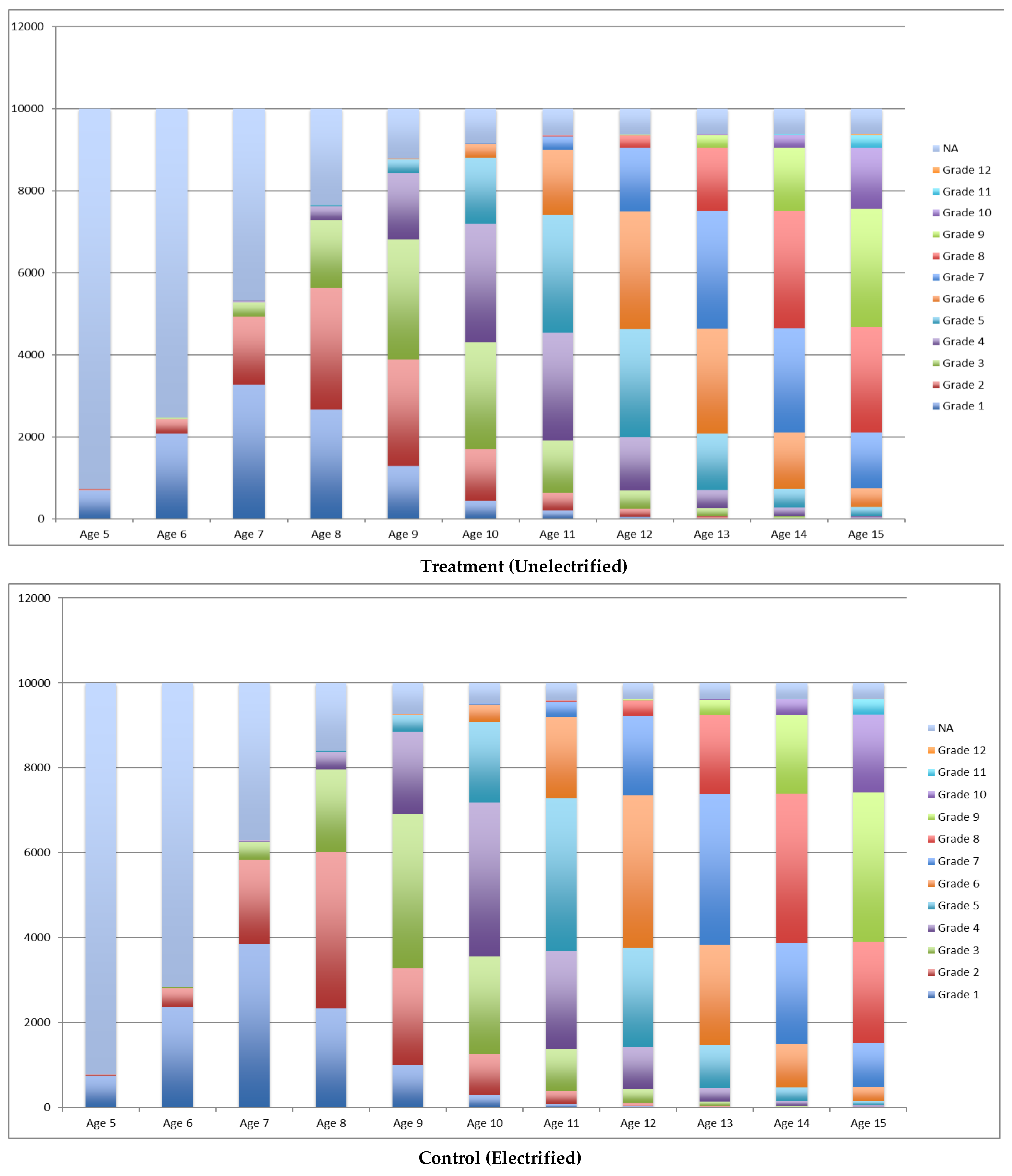
When we examined the transition up to age 15, we obtained the following results (see Figure 1):

Consider a 15-year-old who enrolled in grade 1 at age 5 and will potentially reach grade 12 when he/she is age 15. He/she needs to complete 12 years of school to reach grade 12. This suggests that the treatment can be examined over 10 years based on access to electricity. We can summarize the impact in

Table 8. Long-term impact of access to electricity.

Transition	Treatment (Unelectrified)	Control (Electrified)
Non-attendance	6.17%	3.69%
Grade 11	3.14%	3.57%
Grade 10	14.89%	18.40%
Grade 9	28.73%	35.15%

as follows:

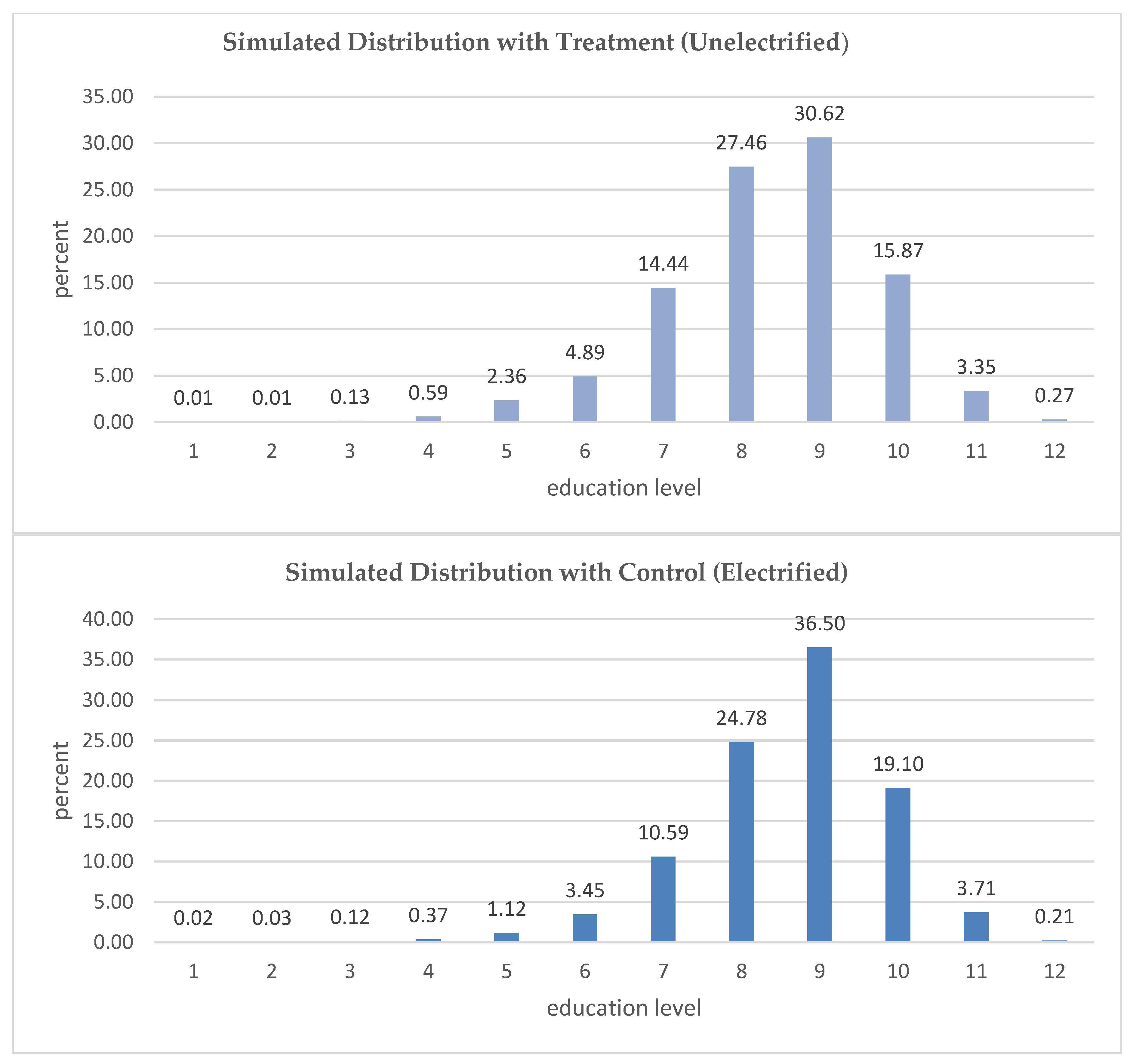
We apply the simulation to estimate the long-term impact of access to electricity. Our simulation assumes that a child is going to school continuously for 10 years, starting at age 5. We compare the predicted school enrollment distribution between the unelectrified (treatment) and electrified (control) groups at age 15 and omit non-attendance students.

Table 9. Simulated school enrollment distribution at age 15 for treatment and control.

Grade	Treatment (PDF)	Control (PDF)	Treatment (CDF)	Control (CDF)
1	0.01	0.02	0.01	0.02
2	0.01	0.03	0.02	0.05
3	0.13	0.12	0.15	0.17
4	0.59	0.37	0.74	0.54
5	2.36	1.12	3.1	1.66
6	4.89	3.45	7.9	5.11
7	14.44	10.59	22.34	15.7
8	27.46	24.78	49.8	40.48
9	30.62	36.50	80.42	76.98
10	15.87	19.10	96.29	96.08
11	3.35	3.71	99.64	99.79
12	0.27	0.21	100	100

presents the simulated probability distribution function (PDF) and cumulative distribution function (CDF) values for the treatment and control, with treatment defined as lacking access to household electricity for 10 years for the age range 5–15.

Figure 2 displays the school enrollment scenario for a 15-year-old child who has continuously attended school for the last 10 years. The school enrollment rate is higher for grades 9–11 in the electrified group compared to the unelectrified group, revealing substantial differences between the treatment and control groups. Most of the treatment impact occurs at age 14.

We predict the long-run impact of access to electricity on education, demonstrating that this is a very strategic policy option for justifying the provision of electricity in unelectrified regions to reduce school non-attendance. We also note that grade progression is affected by the quality of light. The quality of lighting, especially in rural areas, is an important indicator that should be focused on education policy. The quality of lighting provides an opportunity for the learners to study at night. We believe that it can increase school enrollment.

5. Conclusions

In theory, the impact of access to electricity on education is unclear. There may be multiple mechanisms at work. There is no consensus on the empirical literature on the impact of access to electricity on education. This paper documents empirical research that tests the strategic policy question of whether access to electricity increases grade progression and reduces non-attendance rates for children aged between 5 and 15. The relationship between access to electricity and school enrollment is complex. Although access to electricity affects children’s study, it is not the only factor (factors such as income, location, culture, and government policy are also considered very important). The occurrence of non-attendance resulted from a complex interaction of economic, individual, family and school-related factors [41]. There is a positive relationship between access to electricity and economic condition of the household [42]. Our focus point is to assess the impact of electrification on school enrollment. Particularly notable is the impact of access to electricity on grade progression and non-attendance observed in the current study between the treatment and control groups in both the short and long run. Firstly, the average treatment effect on the treated (ATET) showed that access to electricity significantly increased grade progression and reduced non-attendance. Secondly, the Markov schooling transition model showed that access to electricity had a positive impact on grade progression and a negative impact on non-attendance in the short and long run. For grade repetition, however, access to electricity had a mixed effect.

Although some researchers have found positive effects, some have found no effect. In some instances, access to electricity showed some improvement in the number of study hours and school enrollment [43,44]. However, in another case lighting had an insignificant effect on children’s study time [45]. To contribute to the existing literature, we evaluate the impact of access to electricity on grade progression, repetition, and non-attendance. Overall, a broad scope is apparent for enhancing school enrollment by ensuring access to electricity. Education policies are needed to encourage school enrollment and to reduce non-attendance at primary and secondary school based on strategic factors. These policies could provide financial support and quality of lighting, potentially increasing study continuation for children. It is noteworthy to mention that the government can take the initiative to reduce the student non-attendance, which is partially caused by non-access to electricity. One empirical study showed that access to electricity reduces school attendance [46]. Our findings do not support this finding. We found that the quality of lighting can be considered for reducing the non-attendance in Bangladesh. Many characteristics of rural areas make it more challenging (unfeasible and impractical) to provide grid electricity [47]. Improved targeting of educational research and resources on access to lighting and education might be a strong tool for maximizing school enrollment in Bangladesh.

References

- Juslén, H.; Tenner, A. Mechanisms involved in enhancing human performance by changing the lighting in the industrial workplace. Int. J. Ind. Ergon. 2005, 35, 843–855. [Google Scholar] [CrossRef]
- Bellia, L.; Pedace, A.; Barbato, G. Lighting in educational environments: An example of a complete analysis of the effects of daylight and electric light on occupants. Build. Environ. 2013, 68, 50–65. [Google Scholar] [CrossRef]
- Jere, B.R.; Piyali, S.; Petra, T. Progressing through PROGRESA: An impact assessment of a school subsidy experiment in rural Mexico. Econ. Dev. Cult. Chang. 2005, 54, 237–275. [Google Scholar]
- Shyu, C. Energy for sustainable development: Ensuring access to electricity and minimum basic electricity needs as a goal for the post-MDG development agenda after 2015. Energy Sustain. Dev. 2015, 19, 29–38. [Google Scholar] [CrossRef]
- Legros, G.; Havet, I.; Bruce, N.; Bonjour, S. The Energy Access Situation in Developing Countries: A Review Focusing on the Least Developed Countries and Sub-Saharan Africa; World Health Organization (WHO): Geneva, Switzerland; United Nations Development Programme (UNDP): New York, NY, USA, 2009. [Google Scholar]
- Niu, S.; Jia, Y.; Wang, W.; He, R.; Hu, L.; Liu, Y. Electricity consumption and human development level: A comparative analysis based on panel data for 50 countries. Int. J. Electr. Power Energy Syst. 2013, 53, 338–347. [Google Scholar] [CrossRef]
- Reddy, B.S.; Srinivas, T. Energy use in Indian household sector—An actor-oriented approach. Energy 2009, 34, 992–1002. [Google Scholar] [CrossRef]
- Yimen, N.; Hamandjoda, O.; Meva’a, L.; Ndzana, B.; Nganhou, J. Analyzing of a photovoltaic/wind/ biogas/pumped-hydro off-grid hybrid system for rural electrification in Sub-Saharan Africa—Case study of Djoundé in Northern Cameroon. Energies 2018, 11, 2644. [Google Scholar] [CrossRef]
- Bertheau, P.; Oyewo, A.S.; Cader, C.; Breyer, C.; Blechinger, P. Visualizing national electrification scenarios for sub-saharan African countries. Energies 2017, 10, 1899. [Google Scholar] [CrossRef]
- Bridge, B.A.; Adhikari, D.; Fontenla, M. Household-level effects of electricity on income. Energy Econ. 2016, 58, 222–228. [Google Scholar] [CrossRef]
- Bernard, T. Impact analysis of rural electrification projects in Sub-Saharan Africa. World Bank Res. Obs. 2012, 27, 33–51. [Google Scholar] [CrossRef]
- Independent Evaluation Group (IEG). The Welfare Impact of Rural Electrification: A Reassessment of the Costs and Benefits: An IEG Impact Evaluation; IEG: Washington, DC, USA, 2008. [Google Scholar]
- Daka, K.R.; Ballet, J. Children’s education and home electrification: A case study in northwestern Madagascar. Energy Policy 2011, 39, 2866–2874. [Google Scholar] [CrossRef]
- Matinga, M.N.; Annegarn, H.J. Paradoxical impacts of electricity on life in a rural South African village. Energy Policy 2013, 58, 295–302. [Google Scholar] [CrossRef]
- Dinkelman, T. The effects of rural electrification on employment: New evidence from South Africa. Am. Econ. Rev. 2011, 101, 3078–3108. [Google Scholar] [CrossRef]
- Fujii, T.; Shonchoy, A.S.; Xu, S. Impact of electrification on children’s nutritional status in rural Bangladesh. World Dev. 2018, 102, 315–330. [Google Scholar] [CrossRef]
- Khandker, S.R.; Barnes, D.F.; Samad, H.A. Welfare Impacts of Rural Electrification: A Case Study from Bangladesh; WPS4859; The World Bank Group: Washington, DC, USA, 2009. [Google Scholar]
- Lipscomb, M.; Barham, T. Development effects of electrification: Evidence from the topographic placement of hydropower plants in Brazil. Am. Econ. J. Appl. Econ. 2013, 5, 200–231. [Google Scholar] [CrossRef]
- Komatsu, S.; Kaneko, S.; Ghosh, P.P.; Morinaga, A. Determinants of user satisfaction with solar home systems in rural Bangladesh. Energy 2013, 61, 52–58. [Google Scholar] [CrossRef]
- Sovacool, B.K.; Ryan, S.E. The geography of energy and education: Leaders, laggards, and lessons for achieving primary and secondary school electrification. Renew. Sustain. Energy Rev. 2016, 58, 107–123. [Google Scholar] [CrossRef]
- Dasso, R.; Fernandez, F.; Ñopo, H. Electrification and Educational Outcomes in Rural Peru; No. 8928; Institute for the Study of Labor: Bonn, Germany, 2015. [Google Scholar]
- Arends-Kuenning, M.; Amin, S. School incentive programs and children’s activities: The case of Bangladesh. Comp. Educ. Rev. 2004, 48, 295–317. [Google Scholar]
- Ahmed, A.U.; Del Ninno, C. The Food for Education Program in Bangladesh: An Evaluation of Its Impact on Educational Attainment and Food Security; IFPRI: Washington, DC, USA, 2002. [Google Scholar]
- World Bank. Education at a Glance: Bangladesh; The World Bank Group: Washington, DC, USA, 2009. [Google Scholar]
- Taniguchi, K. Determinants of grade repetition in primary school in sub-Saharan Africa: An event history analysis for rural Malawi. Int. J. Educ. Dev. 2015, 45, 98–111. [Google Scholar] [CrossRef]
- Sabates, R.; Hossain, A.; Lewin, K.M. School drop out in Bangladesh: Insights using panel data. Int. J. Educ. Dev. 2013, 33, 225–232. [Google Scholar] [CrossRef]
- Longenecker, E.I.; Barnum, A.J. The problem of secondary education completion: The case study of Cape Verde, a small island developing state. Int. J. Educ. Dev. 2017, 53, 48–57. [Google Scholar] [CrossRef]
- Barron, M.; Torero, M. Household electrification and indoor air pollution. J. Environ. Econ. Manag. 2017, 86, 81–92. [Google Scholar] [CrossRef]
- Bekker, B.; Eberhard, A.; Gaunt, T.; Marquard, A. South Africa’s rapid electrification programme: Policy, institutional, planning, financing and technical innovations. Energy Policy 2008, 36, 3115–3127. [Google Scholar] [CrossRef]
- Abadie, A. Semiparametric instrumental variable estimation of treatment response models. J. Econom. 2003, 113, 231–263. [Google Scholar] [CrossRef]
- James, H.; Salvador, N.-L. Using matching, instrumental variables, and control functions to estimate economic choice models. Rev. Econ. Stat. 2016, 86, 30–57. [Google Scholar]
- Smith, J.A.; Todd, P.E. Does matching overcome LaLonde’s critique of nonexperimental estimators? J. Econom. 2005, 125, 305–353. [Google Scholar] [CrossRef]
- Rosenbaum, P.R.; Rubin, D.B. The central role of the propensity score in observational studies for causal effects. Biometrika 1983, 70, 41–55. [Google Scholar] [CrossRef]
- Heckman, J.J.; Ichimura, H.; Todd, P. Matching as an econometric evaluation estimator. Rev. Econ. Stud. 1998, 65, 261–294. [Google Scholar] [CrossRef]
- Ye, Y.; Koch, S.F.; Zhang, J. Determinants of household electricity consumption in South Africa. Energy Econ. 2018, 75, 120–133. [Google Scholar] [CrossRef]
- Bedir, M.; Hasselaar, E.; Itard, L. Determinants of electricity consumption in Dutch dwellings. Energy Build. 2013, 58, 194–207. [Google Scholar] [CrossRef]
- Ahmad, S.; Mathai, M.V.; Parayil, G. Household electricity access, availability and human well-being: Evidence from India. Energy Policy 2014, 69, 308–315. [Google Scholar] [CrossRef]
- Kanagawa, M.; Nakata, T. Assessment of access to electricity and the socio-economic impacts in rural areas of developing countries. Energy Policy 2008, 36, 2016–2029. [Google Scholar] [CrossRef]
- Khandker, S.R.; Barnes, D.F.; Samad, H.; Minh, N.M. Welfare Impacts of Rural Electrification: Evidence from Vietnam; Policy Research Working Paper; East Asia and Pacific Region, World Bank Sustainable Development: Washington DC, USA, 2009; pp. 1–49. [Google Scholar]
- Kumar, S.; Rauniyar, G. Is Electrification Welfare Improving? Non-Experimental Evidence from Rural Bhutan; University Library of Munich: Munich, Germany, 2011. [Google Scholar]
- Bastein, S. Out-of-school and ‘at risk’?: Socio-demographic characteristics, AIDS knowledge and risk perception among young people in Northern Tanzania. Int. J. Educ. Dev. 2008, 28, 393–404. [Google Scholar] [CrossRef]
- Goldemberg, J.; La Rovere, E.L.; Coelho, S.T. Expanding access to electricity in Brazil. Energy Sustain. Dev. 2004, 8, 86–94. [Google Scholar] [CrossRef]
- Barron, M.; Torero, M. Short Term Effects of Household Electrification: Experimental Evidence from Northern el Salvador; Job Market Paper; IFPRI: Washington, DC, USA, 2014. [Google Scholar]
- Khandker, S.R.; Samad, H.A.; Ali, R.; Barnes, D.F. Who Benefits Most from Rural Electrification? Evidence in India; Working Paper; The World Bank Group: Washington, DC, USA, 2012. [Google Scholar]
- Bensch, G.; Kluve, J.; Peters, J. Impacts of rural electrification in Rwanda. J. Dev. Effect. 2011, 3, 567–588. [Google Scholar] [CrossRef]
- Squires, T. The Impact of Access to Electricity on Education: Evidence from Honduras; Job Market Paper; Brown University: Providence, RI, USA, 2015. [Google Scholar]
- Rahman, M.M.; Paatero, J.V.; Poudyal, A.; Lahdelma, R. Driving and hindering factors for rural electrification in developing countries: Lessons from Bangladesh. Energy Policy 2013, 61, 840–851. [Google Scholar] [CrossRef]
Figure 1.
Grade transition from age 5–15.
Figure 2.
Simulated effects of treatment on school enrollment distribution at age 15.