Mechatronic Modeling and Frequency Analysis of the Drive Train of a Horizontal Wind Turbine


1
Department of Mechanical Engineering, Basque Country University (UPV/EHU), Nieves Cano, 12, 01006 Vitoria-Gasteiz, Spain
2
Department of System Engineering and Automation Control, Basque Country University (UPV/EHU), Nieves Cano, 12, 01006 Vitoria-Gasteiz, Spain
3
Department of Nuclear and Fluid Mechanics, Basque Country University (UPV/EHU), Nieves Cano, 12, 01006 Vitoria-Gasteiz, Spain
*
Author to whom correspondence should be addressed.
Energies 2019, 12(4), 613; https://doi.org/10.3390/en12040613
Submission received: 28 December 2018
/
Revised: 31 January 2019
/
Accepted: 12 February 2019
/
Published: 15 February 2019
(This article belongs to the Special Issue Design, Fabrication and Performance of Wind Turbines 2019)
Abstract
:The relevance of renewable energies is undeniable, and among them, the importance of wind energy is capital. A lot of literature has been devoted to the control techniques that deal with the optimization of the energy produced, but the maintainability of the individual wind turbines and of the farms in general is also a fundamental factor to take into account. In this paper, the authors address the general problem of knowing in advance the resonance frequencies of the power system of a wind turbine, with the underlying idea being that those frequencies should be avoided and that resonances do not occur only due to mechanical phenomena, but also because of electrical phenomena that in turn are influenced by control and optimization techniques. Therefore, the availability of that information embedded in the optimization techniques that control a wind turbine is of major importance. The main purpose of this paper was accomplished through two related objectives: the first was to obtain a mechatronic model (using a lumped parameters model of two degrees of freedom) of the drive train in the Laplace domain oriented to subsequently perform the described analysis. The second was to use that model to determine analytically the number and the value of the resonance frequencies from the generator angular velocity in such a way that such information could be used by any control algorithm or even by the mechatronic system designers. We assessed through experimental validation using a real 100 kW wind turbine that these two objectives were reached, demonstrating that the different vibration modes were detected using only the generator angular velocity.
1. Introduction
Traditionally, automotive, construction, aeronautics, energy, railway, security, and health had some of the most demanding applications in the mechatronic field. In the last decades, fusion and renewable energies (marine platforms, photovoltaic technologies, etc.) have been quickly expanding sectors. More recently in the energy sector, industrial processes such as oil and gas as well as wind energy extraction in renewable energies have become popular. Above all, specifically, wind energy represents a major player in the context of renewable energies, being the most widespread renewable source [1].
Mechanics and control are key issues in any mechatronic application. The drive train is one of the most critical parts of wind turbines, and it is where mechanical and control failures are concentrated. The main objective of wind turbines is to extract the maximum amount of energy from wind [2,3], taking into account both the environmental [4] and economic effects [1,5], and avoiding resonances in the tower and the rest of the structure [6,7]. Mechanical fatigue can cause wear of elements of the nacelle and the tower, which in turn can cause resonances with the consequent breakage of elements, losing power performance and decreasing safety [8]. In the study of Cambron et al. [9], an application about the detection of the imbalance of the rotor describes the vibration and resonances of the tower.
The power system inside the nacelle consists of a slow shaft, a gearbox, and a fast shaft. The axes are supported by their corresponding bearings, and in the fast shaft there is also a flexible coupling to withstand misalignments, as described in Santoso et al. [10]. In order to deal with the previously exposed problems, there are in the literature a number of works related to design, dynamic analysis, vibratory analysis, non-linear analysis, ageing assessment, control analysis, and the analysis of the root-locus in the drive train of variable speed wind turbines.
In terms of design, Nejadkhaki et al. [11] have proposed a design methodology for the selection of ratios in variable gearboxes. Previously, Peeters et al. [12] and Zhu et al. [13] carried out dynamic analysis in wind turbine transmissions, while Todorov et al. [14] focused their study on torsional oscillations of horizontal turbines.
In the power system of a wind turbine there are some elements mechanically more sensitive or elastic than others. For instance, the multiplier and the flexible coupling are the weakest components by their nature [12,14], and their frequencies dominate the natural frequencies of the drive train.
According to Martínez-Lucas [4], an exhaustive study of signals in the time domain or frequency response helps in frequency regulation and, according to Pashazadheh [15], in developing strategies or methods for fault detection. Additionally, Shao et al. [16] proposed a method to develop a fault reconstruction model capable of describing a non-linear real-time process using a parameter updating system. In drive trains that work with variable speeds, the vibratory collected signals are non-stationary and non-linear. Closely related to these issues, in 2017, Maheswari and Umamaheswari [17] reviewed recent research advances studying particularly non-stationary and non-linear signal processing algorithms for variable-speed wind turbines.
It is important to slow down the ageing of wind turbines. Therefore, authors such as Cambron et al. [9] and Dai et al. [18] have supervised and controlled wind turbines using different systems. Dai et al. [18] concluded that the evaluation of ageing is not only effective for optimization and maintenance of operations, but also to improve the management of wind turbine farms.
The power and the pitch loops are the most important loops of a wind turbine. The power loop tries to smooth the fluctuations that a change in wind speed could cause, while the pitch loop tries to maintain a command velocity in the generator [19]. Menezes et al. [1] carried out a detailed review of these two types of loop control currently used in wind turbines.
Wilches-Bernal [20] and later Freijedo et al. [21] carried out an analysis of the root locus to investigate the frequencies of wind turbines. An appropriate frequency regulation control can improve the frequency response of the system. Since wind generation is connected to the grid by means of power electronics, it allows a faster and more flexible control of the output power. Freijedo et al. [21] designed a controller for the pitch system by analyzing the root locus when the wind turbine is unloaded, developing a methodology for the design and adjustment of the current controller and providing a transfer function for the analysis of the root locus.
This paper pursues a double objective. The first is to obtain an accurate model of the drive train of a wind turbine, an objective that has been reached through the two degrees-of-freedom (dof) formalization in the Laplace domain that has been introduced. The second and main objective of the paper is to use the models obtained, following the previous formalization, in order to carry out a dynamic analysis of the power system of a turbine and determine its behavior regarding the resonance frequencies. This objective was also reached and validated through experimental measurements.
The structure of the paper is as follows. In the second section, a dynamic model of the power system of a wind turbine is developed, while in the third section a dynamic analysis of the modeling of the drive train is explained. In the fourth section the model is experimentally validated by means of a frequency analysis. Finally, the last section of the paper summarizes the main conclusions.
2. Dynamic Modeling of the Drive Train
The drive train of wind turbines is the most complex part from the mechatronic, mechanical, and dynamic points of view. Parameters such as inertias and stiffness must be well estimated in the models for an optimal subsequent design of the elements of any mechanism or machine. Many works study the rotor dynamics with very different interests, so their approaches change depending on the objectives of the authors. Some papers are specially oriented to power network stability analysis as in [22,23,24,25,26]. These works are especially interesting because they have deep electrical studies and they use equivalent mechanical train dynamical models with one and two masses [27]. In our case, the generator torque has another law that depends on the actual rotor speed as in [8,28,29].
Traditionally, the modeling alternatives are numerical and analytical. Regarding numerical models, in the scientific literature, the finite element based models predominate [30], but there are also multibody models.
Several authors have modeled mechanisms using analytical methods based on Newton–Euler [31] and Lagrange [32] principles. Within the analytical models, the models of lumped parameters represent symbolically a reduction of point masses that correspond to the inertias of the elements of the mechanism, interacting springs, and dampers [7,12].
Inertial models are the simplest lumped parameter model type, since the system is considered perfectly rigid. They can be useful for the first approximations, but by only considering an over-simplified and ideal system, phenomenon such as vibrations could be neglected.
It is very common to model a mechatronic system using 2-dof models [12,22], for example, machine tool drives [33]. These models of lumped parameters are a simplification of reality because they are simple to pose and the solutions can be parameterized. If the hypothesis of reduction of the model is adequate, very close-to-reality solutions can be obtained with simple models. Normally, these models are used in the first stage of design [34]. In the 2-dof lumped parameter models, a first mass represents the axis of the drive and the input force applied to it, while a second mass represents the mass of the load, where the output movement of the transmission chain is studied. The springs represent the equivalent stiffness between the elements, while the dampers represent the dissipating effects in the components. A model of N dof takes into account the dynamics of more components of the mechatronic system. From a design point of view, N-dof models are very useful because they allow for the carrying out of a detailed modal analysis. Using this kind of model, the component of the system that provides more mechanical instability can be detected and replaced [33].
If very accurate calculations are required or the simplification of the lumped parameter model is excessive and cannot be assumed, the finite element models (FEM) are the most appropriate ones due to their ability to deal with continuous systems analyzing in detail the contact between two different bodies. However, the analysis is complicated when more than one joint between bodies is required. FEMs describe in detail loose bodies, but not kinematic chains, mechanisms, nor machines with different bodies and many joints [30].
Multibody models are used for calculations with good accuracy where dynamic, kinematic, and structural simulations are required. Multibody models are also called cosimulation or COSIM.
Depending on the objectives of the analysis and how the power system of a wind turbine is configured, a model of lumped parameters could be chosen to perform the dynamic analysis. In the model analysis carried out by Ansoategui et al. [33], two conclusions were reached. Firstly, if the purpose is to simulate the dynamic behavior of the system, then it is enough to use a model of 2 dof since it collects the first vibration mode, which will limit the bandwidth of the control loop. Secondly, if the purpose is to redesign, then the model of N dof is better because it can predict which element is weak.
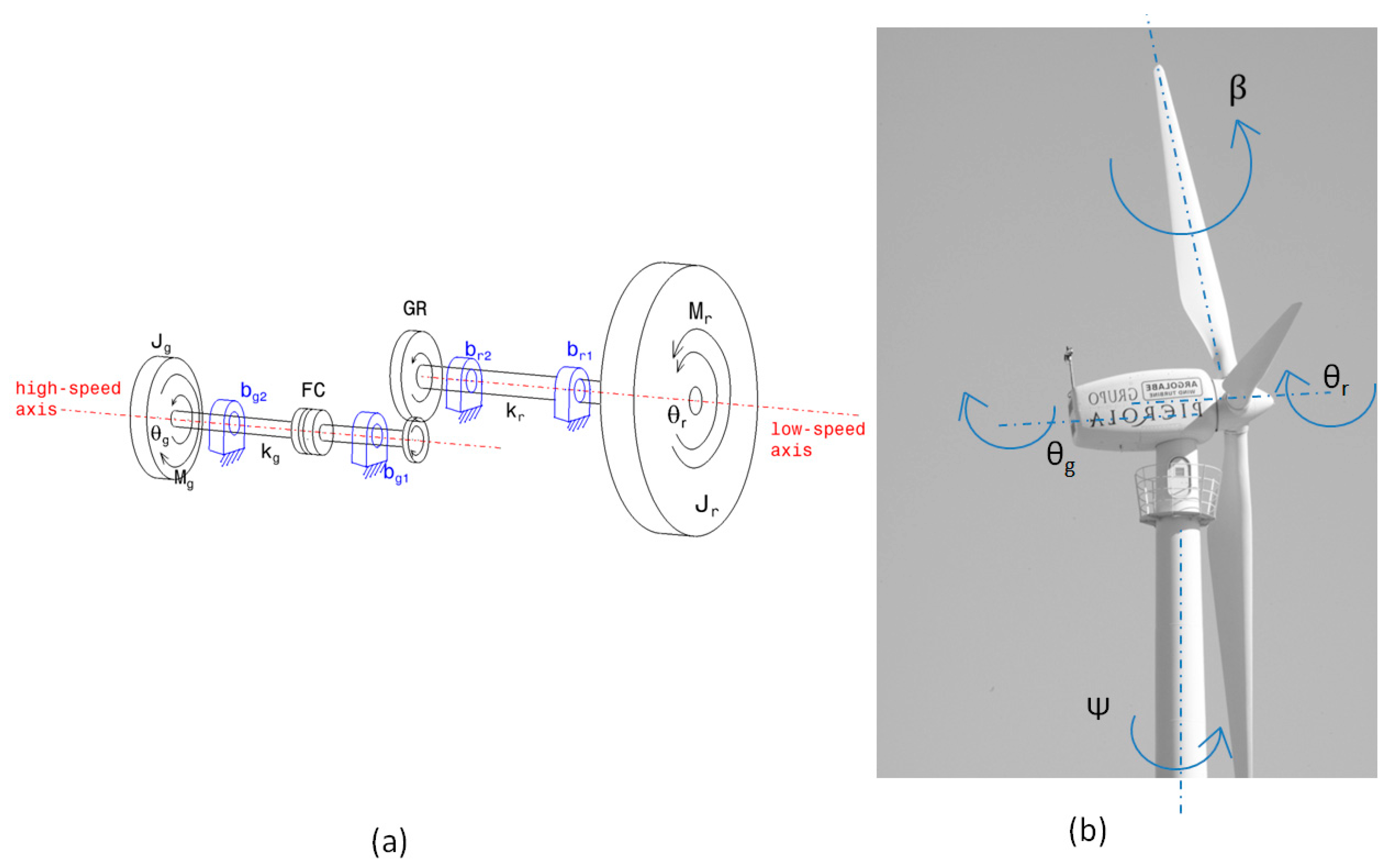
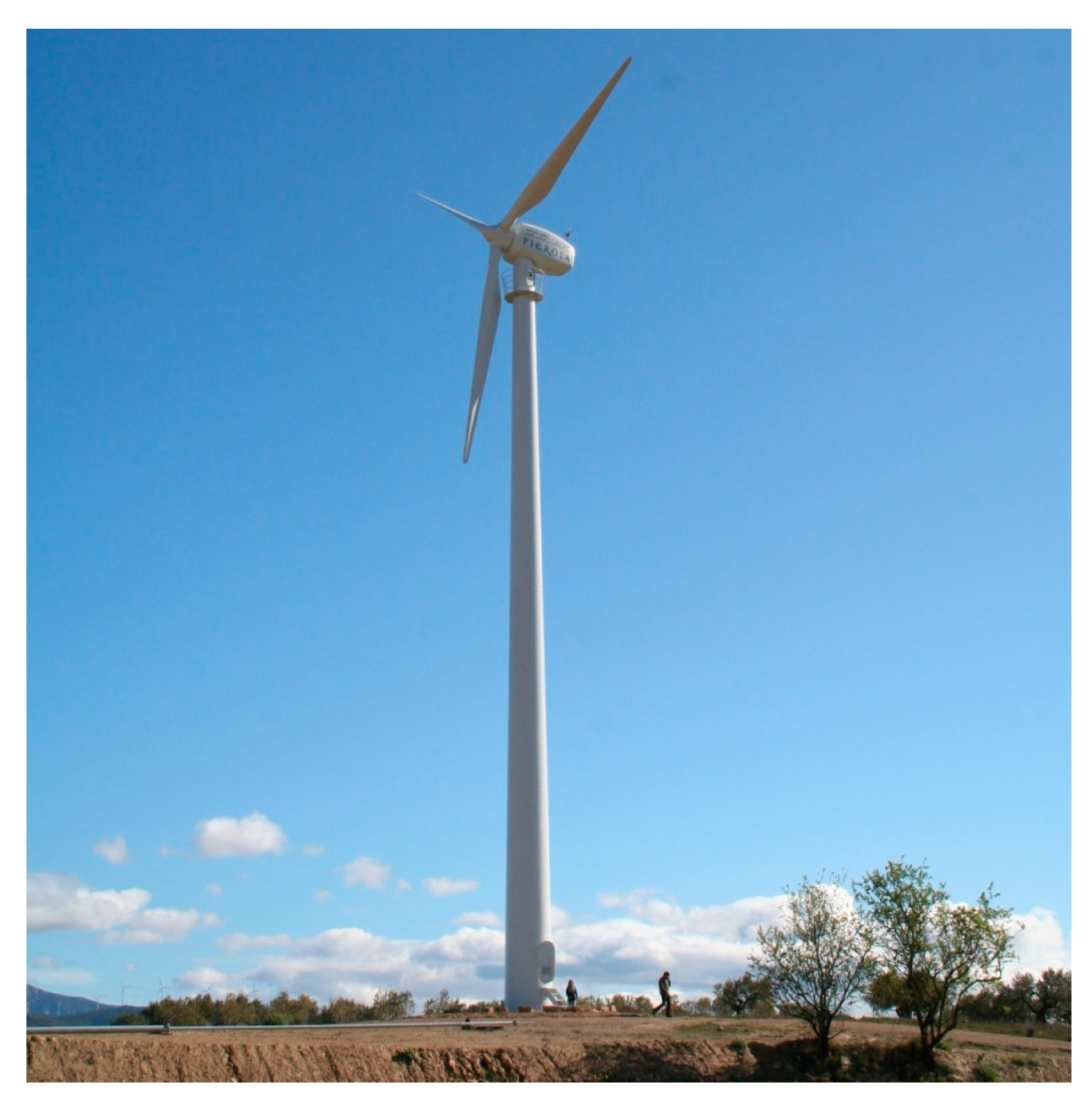
The experimentation of this paper is carried out in a 100-kW wind turbine of the Argolabe S.L. Engineering Company, shown in Figure 1b. A sketch of the drive train of that wind turbine is shown in Figure 1a.
The main movements to be managed by a wind turbine control are the pitch movement of the blades (β) and the yaw movement of the nacelle (Ψ), represented in Figure 1b.
As for the drive train, the main axes are the slow axis or the rotor axis (θr), and the fast axis or the generator axis (θg). Figure 1a represents the mechanical elements of the power system: rotor, multiplier (GR), flexible coupling (FC), and generator. The slow and fast axes are supported by their corresponding bearings. The slow shaft is supported by the bearings br1 and br2, which are characterized by a specific damping coefficient [N·m·s/rad], and the fast shaft by bg1 and bg2. The stiffness values of the slow and the fast axes of the rotor are defined as kr and kg [N·m/rad], respectively.
The gearbox of the wind turbine consists of two pairs of helical gears with axes arranged in parallel. The flexible coupling attached to the quick shaft will absorb misalignments between axes caused by design, assembly, or operation. In the multiplier, labeled GR in Figure 1a and composed of a pair of gears, the non-linearities caused by backlash between the teeth are present while the mechanism is working.
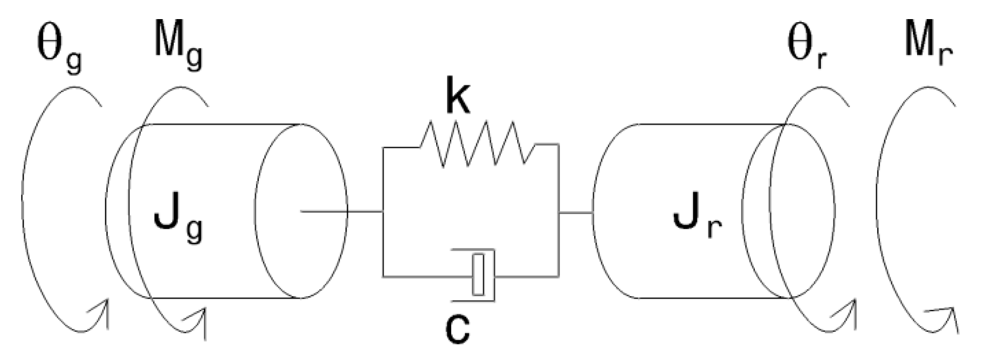
Given that one of the main purposes of this paper is to develop and validate a mechatronic model of the power system of a wind turbine (represented in Figure 2), the chosen approach is based on a model of lumped parameters of 2 dof developed by Martins et al [31]. In Figure 2, Mr [N·m] represents the moment of the rotor axis and Mg the moment of the generator, while Jr and Jg [kg·m2] represent the inertia of the rotor and the generator, respectively. Finally, k [N·m/rad] and c [N·m·s/rad] correspond to the equivalent stiffness and damping of the power train.
Developing a free solid diagram analysis of the bodies of Figure 2, the equations of motion corresponding to the 2-dof model are described in the Laplace domain in Equation (1):
Since the arrangement of the bodies and joints is a chain of transmission in series as shown in Figure 1a, the equivalent rigidity k [N·m/rad] of the system is defined by Equation (2), considering the rigidity of the rotor kr and the generator kg:
The electrical machine of this wind turbine is a synchronous one. This electrical machine has power electronics, and these electronics have their own torque-control loop. This control loop is a vector control one, therefore, our control law gives to these electronics a torque set point. The power electronics can impose the torque set point very quickly, in fact, the time constant of this torque loop is less than 8 × 10⁻³ s. Keeping this in mind, the torque-loop dynamics are almost negligible compared to mechanical-dynamics time constants. Then, the torque set point and the generator torque can be linked by the differential equation expressed as a transfer function of Equation (3):
where τpe [s] is the time constant of the power stage, Msp is torque set point, and Mg is the generator torque. Finally, we recall that the generator torque follows a quadratic mathematical law in order to achieve the maximum power point. Therefore, the power set point Msp is equivalent to Equation (4):
where the torque set point Msp is calculated as a function of the air density ρ [kg/m3], the radius of the blades R [m], the optimal Tip-Speed Ratio (TSR) λopt [rad], the angular velocity of the generator ωg [rad/s], and the maximum power coefficient cp_max [%], as given by Equation (4). The power setpoint Msp can also be calculated as a function of the turbine gain kt and the angular velocity of the generator as indicated in Equation (4).
The control exerts a resistance, therefore, an increment of the torque in the generator ΔMg is assumed. To relate the increase of the generator pair with the set point pair as expressed in Equation (3), the Msp of the Equation (4) is first derived as a function of the angular velocity of the generator. This mathematical development and the resistance phenomenon is expressed in Equation (5)
where kn [kg∙m2/rad∙s] corresponds to the linearization gain. The linearization gain kn represents the slope of the generator torque curve Mg versus the angular velocity of the generator ωg.
The value of the linearization gain kn is proportional to the gain of the turbine kt, the angular velocity of the generator ωg, and a constant, as indicated in the Equation (6).
In order to make a frequency analysis, the damping effect has been neglected. Thus, the parameter c of the Equation (1) has been omitted, being c = 0.
If the equations of motion represented in Equation (1) are expanded taking into account the opposition of the control and the growth of the generator pair defined in Equation (5), then the position of the generator is obtained through Equation (6):
According to Equation (6), it is observed that the angular position of the generator depends on the mechanical properties of the transmission chain. The first term corresponds to the aerodynamic effect, while the second one to the resistance of the control. Deriving Equation (6) in the Laplace domain, i.e., carrying out the operation ωg = θg · s, the angular velocity of the wind turbine generator is obtained as given by Equation (7):
Thus, the global transfer function of the transmission chain of the power system is described in Equation (8):
3. Analysis of the Dynamic Modeling of the Drive Train
Once the transfer function that represents the dynamics of the drive train of a horizontal wind turbine has been found, an analytical study can be carried out with the final aim of providing further insight into the apparition of different resonance frequencies. The starting point is to perform an analysis of the root locus in order to study the stability of the whole system, and for that purpose the denominator of the polynomial transfer function of Equation (8) is expressed by means of the polynomials A(s) and B(s), represented in Equation (9):
To perform a root analysis, the denominator of Equation (8) must be zero as indicated by Equation (10):
Therefore, the linearization gain is expressed by Equation (11):
In the study of dynamic systems, linearization is a method used to study the local stability of a point of equilibrium of a system represented by non-linear differential equations. Basically, it is the process of finding the linear approximation to a function at a given point. In our case, the objective is to linearize the gain kn in order to obtain the critical value of the rotation velocity of the generator, i.e., the value of the rotation velocity from which there is a change in the behavior of the whole system due to changes in the resonance frequencies. Therefore, the linearization of the gain kn fulfills the linearization principle, expressed by the polynomial relation of Equation (12):
The derivative of kn with respect to the variable of Laplace s gives the value of the breakpoint (scritical), which is important in finding the critical value of the rotation velocity of the drive train. Breakpoints are double poles or zeros that override both the denominator and its derivative. When there are trajectories between two real poles or two real zeros, there are breakpoints in which the roots locus leaves the real axes, becoming complex and increasing the number of resonance frequencies. In our case, these transition points are especially important due to the limitations that a resonance imposes in a rotator axis.
Considering the value of the Laplace variable scritical at that breakpoint, the critical linearization gain kn_critical is calculated through Equation (13):
Once the value of the critical linearization gain kn_critical has been obtained and taking into account its fundamental value defined in Equation (4), the value of the generator critical angular velocity is defined by Equation (14):
Since it is known that there is a breakpoint at the value of angular velocity of the generator ωg_critical given by Equation (14), it can be used to deduce analytically whether there will be one or two different resonance frequencies, as given by the algorithm of Equation (15):
4. Experimental Validation
For the experimental validation of the mechatronic model obtained in Section 2 and its dynamic analysis developed in Section 3, theoretical results are studied by comparing them with the experimental results obtained in a real wind turbine. To that purpose, in Section 4.1, the theoretical results are obtained, while Section 4.2 deals with the experimental results.
4.1. Modeling Results
In this section, the theoretical dynamic analysis of Section 3 is instantiated for a real case based on a mechatronic model obtained as outlined in Section 2. In short, the main steps of the pipeline are as follows: (1) The obtained model for the specific real case is formulated as indicated by the transfer function of Equation (8), where the angular velocity of the generator is related to the moment of the rotor produced by the wind. (2) The denominator is split into two polynomials A(s) and B(s) that are used to perform a root locus analysis that helps to obtain the critical value of the angular velocity of the generator, i.e., the angular velocity that determines whether there are one or two resonance frequencies. (3) Finally, a frequency analysis is done with the global transfer function using a Bode diagram to determine such resonance frequency values.
The mechatronic parameters of the 100-kW horizontal-axis wind turbine of Argolabe S.L. Engineering Company are summarized in Table 1, as this is the specific facility where the obtained model was validated from both theoretical and experimental points of view.
To obtain the values of the turbine gain kt introduced in Equation (5), it is mandatory to know the air density, the radius of the blades, the optimal TSR, and the coefficient of the maximum power; these parameters are shown in Table 2.
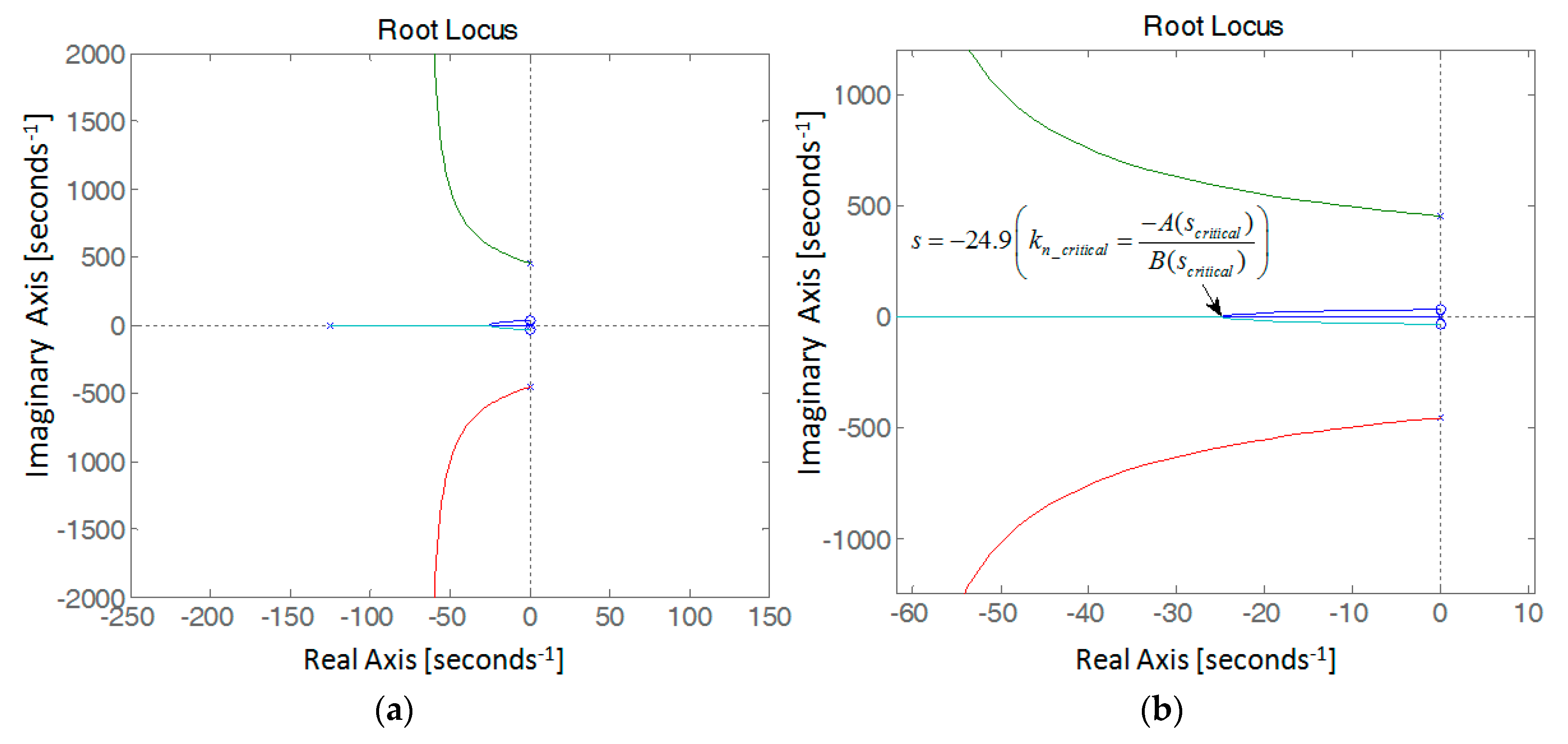
The parameters of Table 1 were used to obtain the mechatronic model of the transmission chain of the power system as indicated by Equation (8), in order to obtain the root locus shown in Figure 3.
The root locus of Figure 3a shows that the obtained system is stable with complex and real roots, therefore, it could have more than one resonance frequency. A zoom-in of the most interesting zone of the root locus is shown in Figure 3b, where it is possible to see that the breakpoint is located at s = −24.9 (so scritical = −24.9), and by substituting that value into Equation (13), the linearization gain value kn_critical for that critical point is determined. The next step is to calculate kt using the values of the parameters of Table 2 in Equation (5). Finally, with the obtained values of kt and kn_critical, the value of ωg_critical is calculated as indicated in Equation (14), giving a critical rotational velocity of ωg_critical = 566.72 rpm.
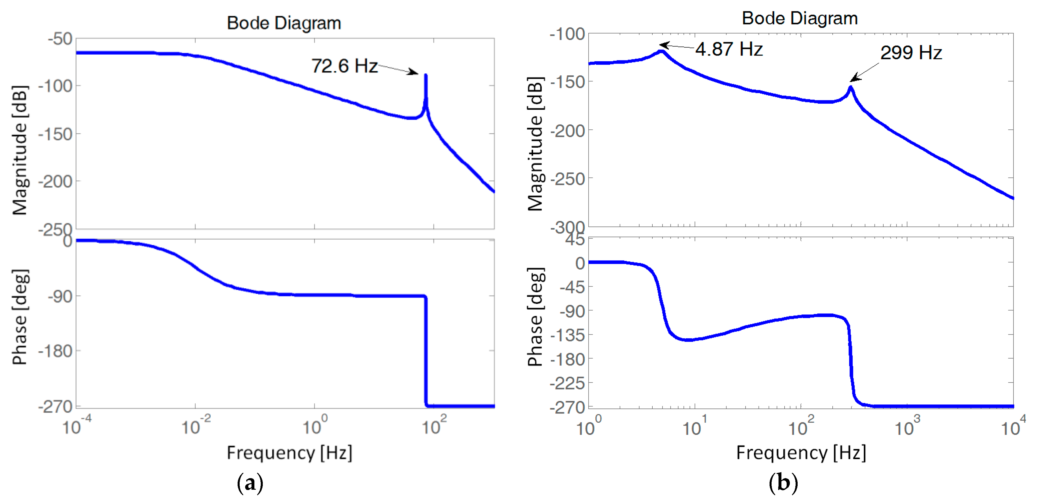
Once the critical rotational velocity of the generator was determined, we carried out a frequency analysis of the model obtained for this real case at two different rotational velocities in order to analyze the frequency behavior of the system regarding the determined value of ωg_critical. For the case of (ωg < ωg_critical), we used a generator fast axis rotation velocity value ωg = 502 rpm obtaining a resonance frequency at 72.6 Hz, as shown in Figure 4a. On the other hand, for the case of (ωg ≥ ωg_critical), a value of ωg = 650 rpm was used obtaining in Figure 4b two different resonance frequencies at 4.87 Hz and 299 Hz, respectively.
It is possible to conclude that following the analytical procedure introduced in Section 3, at least the number of the resonance frequencies of a system modeled following the procedure given in Section 2 can be determined. At this point, it is still mandatory to verify the procedure in a real wind turbine.
4.2. Experimetal Results
Once the procedure to determine the number of the resonance frequencies of the transmission chain of a horizontal wind turbine was analytically validated, we needed to experimentally validate both the mechatronic modeling introduced in Section 2 and the analytical procedure to determine the number of resonance frequencies introduced in Section 3. For that purpose, an experiment was designed using the real 100-kW wind turbine shown in Figure 5.
At a conceptual level, Figure 1a shows that the power system is composed of a rotor, multiplier, flexible coupling, and generator. In this real installation, the gearbox of the wind turbine consists of two pairs of helical gears with axes arranged in parallel; specifically, it is the Rossi brand model R2I280. The transmission ratio between gears is 22:2 and its construction is type B3. The inertia of the reduction gearbox is between 0.0567 and 0.0755 kg·m2. The flexible coupling attached to the quick shaft absorbs misalignments between axes caused by design, assembly, or operation. The rotation velocities of the transmission chain are between 50 and 1,100 rpm. The output torque is 1,000 N·m and the input torque is 22 N·m. Finally, the nominal power of the wind turbine of the Argolabe S.L. Engineering Company is 100 kW.
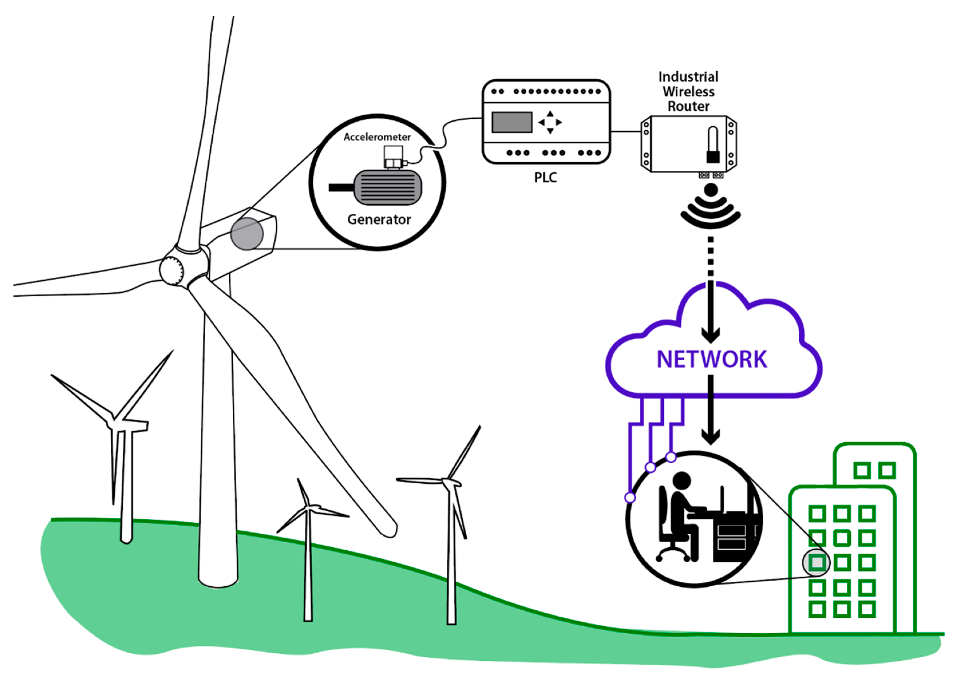
In order to experimentally validate the mechatronic model and perform an optimum frequency analysis, an accelerometer was placed in the transmission chain of the wind turbine of Figure 5, specifically in the generator as indicated in Figure 6. The spectral signals collected by the accelerometer were gathered by a Programmable Logic Device (PLC) and, by means of a wireless industrial router, the signals were sent to the company Argolabe S.L. Engineering Company to be analyzed, as indicated by the pipeline of Figure 6.
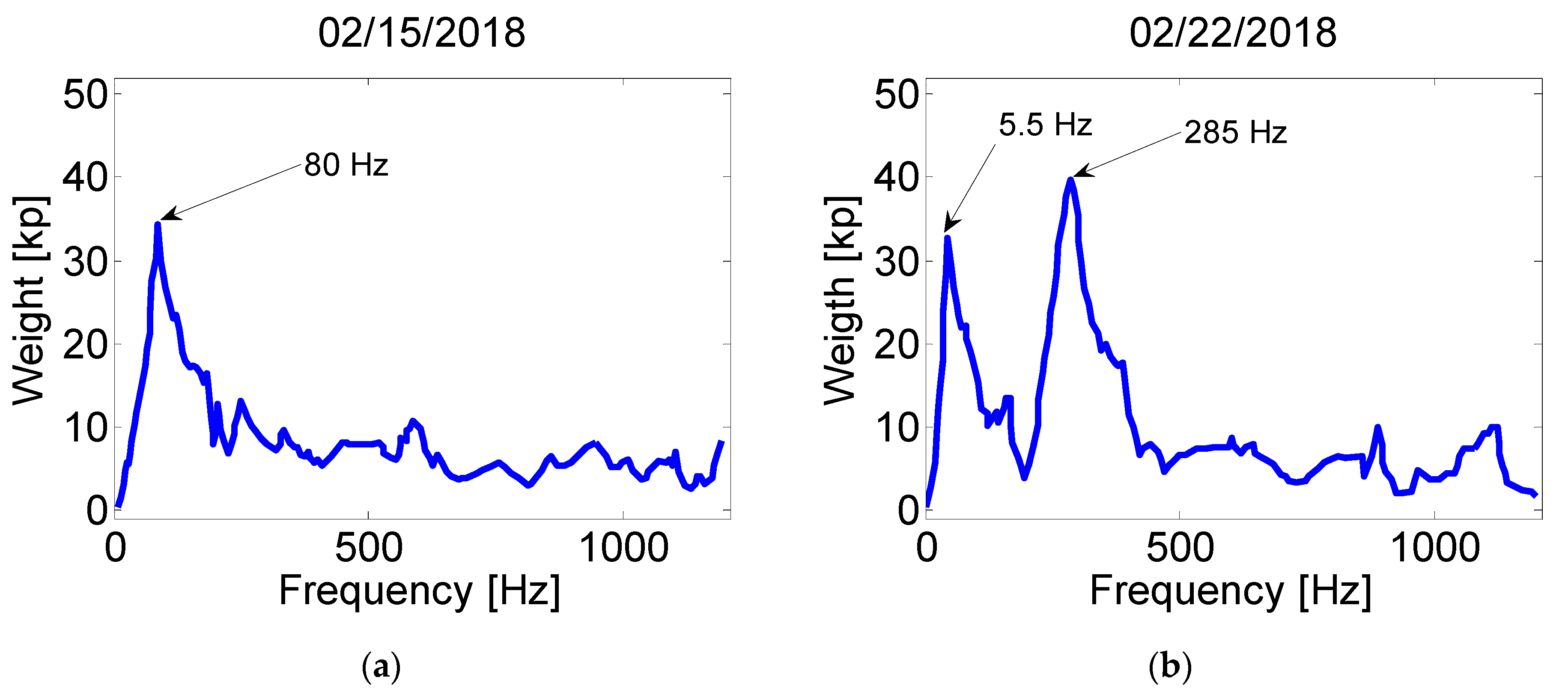
For 30 days the vibratory signals were registered. Frequency analysis, similar to that represented in Figure 4, was completed and the results are shown in Figure 7. These frequency response signals (FRF-s) were sampled by a frequency analyzer that gathered data blocks of 5 s with a 2 kHz sampling time, storing 10,000 samples during the 5 s. One such block was taken every 10 s, so there were 5 s between two consecutive blocks. The frequency signals of Figure 7a and Figure 7b represent the magnitude of weight [kp] versus frequency [Hz] of the sampled measurements, taken in real time during different days.
The data from 15 February 2018 and 22 February 2018 were used for the testing. The reason for selecting these days is that during these days there were angular velocities similar to those of the simulation described in Section 4.1, as such, it was possible to asses that similar resonance frequencies were achieved, validating experimentally the mechatronic model and the conditions of Equation (15).
In the case of Figure 7a, a resonance peak at 80 Hz stands out when ωg ≈ 500 rpm, while in the second case two different resonances arise at approximately 5.5 Hz and at 285 Hz when ωg ≈ 645 rpm, as shown in Figure 7b. Taking into account that for this specific wind turbine ωg_critical = 566.72 rpm, it is possible to see that the values of the experimentally obtained resonance frequencies are very similar to those obtained in Section 4.1 for the two cases specified in Equation (15), and the ωg were not exactly the same in both theoretical and empirical analysis. Therefore, we can conclude that the experimental result validated the procedure introduced in Section 3.
In order to calculate the natural frequencies of the system, we found three main reasons to apply null damping coefficients. (1) We calculated the linear dynamics without damping because damping introduces many more terms in the equations. (2) Damping is not necessary to explain the effect that we want to show. Therefore, we introduced the minimal aspects required to model the effect of one or two resonance frequencies depending on generator speed. (3) Finally, we know that the damping coefficients are not easy to estimate. The difference between the estimated resonance frequency (72.6 Hz) and the real one (80 Hz) was due to non-linear effects rather than linear damping effects, because it is known that the linear damping reduces the resonance amplitude and its resonance frequency.
There are many comprehensive descriptions where the characteristics and non-linear effects that should be taken into account in any mechanism are enumerated, with [35] and [36] being drive trains a specific cases. In any wind turbine drive train, the effect that causes the greatest non-linearity is related to the friction force. The results of Zhou et al. [37] show that the friction force could increase the amplitude of the vibration and seriously affect the low frequency components. It is not easy to carry out the friction compensation, in fact, it still is an open research topic [38]. More non-linear effects could be caused by the backlash and aging of the components and by the eccentricity of the gears of the gearbox.
5. Conclusions
This paper focused on the importance of a good vibratory analysis of the drive trains of wind turbines from two points of view, i.e., to prevent individual wind turbines from ageing and to improve the management of wind turbine farms. The current literature was reviewed, paying more attention to those references that remark on the importance of a frequency analysis. A number of different methods to model mechatronic systems were described, covering different levels of both accuracy and complexity. Then, a novel model for the drive train was introduced, fulfilling the first main objective of the paper. In order to achieve the second main objective, the introduced model was subsequently the subject of a dynamic analysis to determine analytically the number and the value of resonance frequencies of the whole system. For that task, the root locus of the transfer function was obtained, formalizing the concepts of linearization gain and critical generator angular velocity, i.e., the value from which there are not one but two different resonance frequencies.
The theoretical part of the paper, i.e., obtaining the mechatronic model and the dynamic analysis to determine the vibration mode, was validated through an experimental design with a real 100-kW wind turbine. The first step was to obtain the model of the real drive train using its design mechatronic parameters, and after performing a root locus analysis and determining the critical generator angular velocity value, two different generator angular velocities (smaller and larger than that critical value) were used to assess the discriminating capability of such values. The experimental results based on the frequency signals gathered from the real drive train coincide with those determined analytically (in both the number and the value of the resonance frequencies). Therefore, it is possible to conclude that the introduced modeling approach and the subsequent dynamic analysis can be used to perform a frequency analysis of the drive train of a wind turbine.
This kind of analysis is very interesting because the resonances do not occur only by mechanical phenomena, but also by electrical ones that are influenced by the linearization gain (kn) and the constant time (τpe), since the control also influences the dynamics of the transmission chain. Developing a mechatronic model of the wind turbine drive train helps to control the angular velocity and the torque of the generator in such a way that the natural frequencies of the system are not excited.
Author Contributions
Conceptualization, I.A., E.Z., U.F., and J.M.L.G.; data curation, I.A.; formal analysis I.A. and E.Z.; funding acquisition, U.F.; investigation, I.A. and E.Z.; methodology, I.A. and E.Z.; software, I.A. and E.Z.; validation, I.A.; visualization, I.A.; writing—original draft preparation, I.A.; writing—review and editing, U.F. and J.M.L.G.
Funding
The funding from the Government of the Basque Country and the University of the Basque Country UPV/EHU through the SAIOTEK (S-PE11UN112) and EHU12/26 research programs, respectively, is gratefully acknowledged.
Acknowledgments
We appreciate the technical support provided by the Argolabe S.L. Engineering Company.
Conflicts of Interest
The authors declare no conflict of interest.
References
- Menezes, E.J.N.; Araújo, A.M.; da Silva, N.S.B. A review on wind turbine control and its associated methods. J. Clean. Prod. 2018, 174, 945–953. [Google Scholar] [CrossRef]
- El-Hendawi, M.; Gabbar, H.; El-Saady, G.; Ibrahim, E.-N. Control and EMS of a Grid-Connected Microgrid with Economical Analysis. Energies 2018, 11, 129. [Google Scholar] [CrossRef]
- Asghar, M.; Nasimullah. Performance comparison of wind turbine based doubly fed induction generator system using fault tolerant fractional and integer order controllers. Renew. Energy 2018, 116, 244–264. [Google Scholar] [CrossRef]
- Martínez-Lucas, G.; Sarasúa, J.; Sánchez-Fernández, J. Frequency Regulation of a Hybrid Wind–Hydro Power Plant in an Isolated Power System. Energies 2018, 11, 239. [Google Scholar] [CrossRef]
- Uchida, T. LES Investigation of Terrain-Induced Turbulence in Complex Terrain and Economic Effects of Wind Turbine Control. Energies 2018, 11, 1530. [Google Scholar] [CrossRef]
- Castellani, F.; Astolfi, D.; Becchetti, M.; Berno, F.; Cianetti, F.; Cetrini, A. Experimental and Numerical Vibrational Analysis of a Horizontal-Axis Micro-Wind Turbine. Energies 2018, 11, 456. [Google Scholar] [CrossRef]
- Bajrić, A.; Høgsberg, J.; Rüdinger, F. Evaluation of damping estimates by automated Operational Modal Analysis for offshore wind turbine tower vibrations. Renew. Energy 2018, 116, 153–163. [Google Scholar] [CrossRef]
- González-González, A.; Etxeberria-Agiriano, I.; Zulueta, E.; Oterino-Echavarri, F.; Lopez-Guede, J. Pitch Based Wind Turbine Intelligent Speed Setpoint Adjustment Algorithms. Energies 2014, 7, 3793–3809. [Google Scholar] [CrossRef]
- Cambron, P.; Masson, C.; Tahan, A.; Pelletier, F. Control chart monitoring of wind turbine generators using the statistical inertia of a wind farm average. Renew. Energy 2018, 116, 88–98. [Google Scholar] [CrossRef]
- Santoso, S.; Le, H.T. Fundamental time–domain wind turbine models for wind power studies. Renew. Energy 2007, 32, 2436–2452. [Google Scholar] [CrossRef]
- Nejadkhaki, H.K.; Chaudhari, S.; Hall, J.F. A design methodology for selecting ratios for a variable ratio gearbox used in a wind turbine with active blades. Renew. Energy 2018, 118, 1041–1051. [Google Scholar] [CrossRef]
- Peeters, J.L.M.; Vandepitte, D.; Sas, P. Analysis of internal drive train dynamics in a wind turbine. Wind Energy 2006, 9, 141–161. [Google Scholar] [CrossRef]
- Zhu, C.; Chen, S.; Song, C.; Liu, H.; Bai, H.; Ma, F. Dynamic analysis of a megawatt wind turbine drive train. J. Mech. Sci. Technol. 2015, 29, 1913–1919. [Google Scholar] [CrossRef]
- Todorov, M.; Drobrev, I.; Massouh, F. Analysis of Torsional Oscillation of the Drive Train in Horizontal-Axis Wind Turbine. In Proceedings of the ELECTROMOTION 2009, Lille, France, 1–3 July 2009. [Google Scholar]
- Pashazadeh, V.; Salmasi, F.R.; Araabi, B.N. Data driven sensor and actuator fault detection and isolation in wind turbine using classifier fusion. Renew. Energy 2018, 116, 99–106. [Google Scholar] [CrossRef]
- Shao, H.; Gao, Z.; Liu, X.; Busawon, K. Parameter-varying modelling and fault reconstruction for wind turbine systems. Renew. Energy 2018, 116, 145–152. [Google Scholar] [CrossRef]
- Maheswari, R.U.; Umamaheswari, R. Trends in non-stationary signal processing techniques applied to vibration analysis of wind turbine drive train—A contemporary survey. Mech. Syst. Signal Process. 2017, 85, 296–311. [Google Scholar] [CrossRef]
- Dai, J.; Yang, W.; Cao, J.; Liu, D.; Long, X. Ageing assessment of a wind turbine over time by interpreting wind farm SCADA data. Renew. Energy 2018, 116, 199–208. [Google Scholar] [CrossRef]
- Lan, J.; Patton, R.J.; Zhu, X. Fault-tolerant wind turbine pitch control using adaptive sliding mode estimation. Renew. Energy 2018, 116, 219–231. [Google Scholar] [CrossRef]
- Wilches-Bernal, F.; Chow, J.H.; Sanchez-Gasca, J.J. A Fundamental Study of Applying Wind Turbines for Power System Frequency Control. IEEE Trans. Power Syst. 2016, 31, 1496–1505. [Google Scholar] [CrossRef]
- Freijedo, F.D.; Rodriguez-Diaz, E.; Golsorkhi, M.S.; Vasquez, J.C.; Guerrero, J.M. A Root-Locus Design Methodology Derived from the Impedance/Admittance Stability Formulation and Its Application for LCL Grid-Connected Converters in Wind Turbines. IEEE Trans. Power Electron. 2017, 32, 8218–8228. [Google Scholar] [CrossRef]
- Tsourakis, G.; Nomikos, B.M.; Vournas, C.D. Effect of wind parks with doubly fed asynchronous generators on small-signal stability. Electr. Power Syst. Res. 2009, 79, 190–200. [Google Scholar] [CrossRef]
- Eisa, S.A. Modeling dynamics and control of type-3 DFIG wind turbines: Stability, Q Droop function, control limits and extreme scenarios simulation. Electr. Power Syst. Res. 2019, 166, 29–42. [Google Scholar] [CrossRef]
- Eisa, S.A.; Stone, W.; Wedeward, K. Mathematical Modeling, Stability, Bifurcation Analysis, and Simulations of a Type-3 DFIG Wind Turbine’s Dynamics with Pitch Control. In Proceedings of the 2017 Ninth Annual IEEE Green Technologies Conference (GreenTech), Denver, CO, USA, 29–31 March 2017; pp. 334–341. [Google Scholar]
- Eisa, S.A.; Wedeward, K.; Stone, W. Sensitivity Analysis of a Type-3 DFAG Wind Turbine’s Dynamics with Pitch Control. In Proceedings of the 2016 IEEE Green Energy and Systems Conference (IGSEC), Long Beach, CA, USA, 6–7 Noveber 2016. [Google Scholar]
- Eisa, S.A.; Wedeward, K.; Stone, W. Wind turbines control system: nonlinear modeling, simulation, two and three time scale approximations, and data validation. Int. J. Dyn. Control 2018, 6, 1776–1798. [Google Scholar] [CrossRef]
- Clark, K.; Miller, N.W.; Sanchez-Gasca, J.J. Modeling of GE Wind Turbine-Generators for Grid Studies; General Electric International, Inc.: Hong Kong, China, 2010. [Google Scholar]
- Hansen, M.H.; Hansen, A.; Larsen, T.J.; Øye, S.; Sørensen, P.; Fuglsang, P. Control Design for a Pitch-Regulated, Variable Speed Wind Turbine; DTU Library, Riso National Laboratory: Roskilde, Denmark, 2005; ISSN 0106-2840; ISBN 87-550-3409-8. [Google Scholar]
- Hansen, M.O.L. Aerodynamics of Wind Turbines, 3rd ed.; Earthscan: London, UK, 2015; ISBN 978-1-317-67103-9. [Google Scholar]
- Peeters, M.; Santo, G.; Degroote, J.; van Paepegem, W. High-fidelity finite element models of composite wind turbine blades with shell and solid elements. Compos. Struct. 2018, 200, 521–531. [Google Scholar] [CrossRef]
- Martins, M.; Perdana, A.; Ledesma, P.; Agneholm, E.; Carlson, O. Validation of fixed speed wind turbine dynamic models with measured data. Renew. Energy 2007, 32, 1301–1316. [Google Scholar] [CrossRef]
- Chizfahm, A.; Yazdi, E.A.; Eghtesad, M. Dynamic modeling of vortex induced vibration wind turbines. Renew. Energy 2018, 121, 632–643. [Google Scholar] [CrossRef]
- Ansoategui, I.; Campa, F.J. Mechatronics of a ball screw drive using an N degrees of freedom dynamic model. Int. J. Adv. Manuf. Technol. 2017, 93, 1307–1318. [Google Scholar] [CrossRef]
- Ansoategui, I.; Campa, F.J.; López, C.; Díez, M. Influence of the machine tool compliance on the dynamic performance of the servo drives. Int. J. Adv. Manuf. Technol. 2016, 90, 2849–2861. [Google Scholar] [CrossRef]
- Armstrong-Hélouvry, B.; Dupont, P.; de Wit, C.C. A Survey of Models, Analysis Tools and Compensation Methods for the Control of Machines with friction. Automatica 1994, 30, 1083–1138. [Google Scholar] [CrossRef]
- Wit, C.D.C.; Åström, K.J.; Fixot, N. Computed torque control via a non-linear observer. Int. J. Adapt. Control Signal Process. 1990, 4, 443–452. [Google Scholar]
- Zhou, S.; Song, G.; Sun, M.; Ren, Z. Nonlinear dynamic response analysis on gear-rotor-bearing transmission system. J. Vib. Control 2018, 24, 1632–1651. [Google Scholar] [CrossRef]
- Cheng, F.; Zhou, B.; Zhang, L. Wind turbine simulator based on DSEM. In Proceedings of the 2009 IEEE 6th International Power Electronics and Motion Control Conference, Wuhan, China, 17–20 May 2009; pp. 2291–2294. [Google Scholar]
Figure 1.
Argolabe S.L. Engineering Company Wind Turbine: (a) Drive train of the power system; (b) Picture of the wind turbine with the main axes.
Figure 1.
Argolabe S.L. Engineering Company Wind Turbine: (a) Drive train of the power system; (b) Picture of the wind turbine with the main axes.

Figure 2.
Two-dof lumped-parameters model of the drive train.

Figure 3.
(a) Root locus of the power system transmission model; (b) Details of the root locus.

Figure 4.
Bode diagram of the mechatronic model of the power chain of the 100-kW wind turbine. (a) Case of one resonance peak, when ωg = 502 rpm, (b) Case of two resonance peaks, when ωg = 650 rpm.
Figure 4.
Bode diagram of the mechatronic model of the power chain of the 100-kW wind turbine. (a) Case of one resonance peak, when ωg = 502 rpm, (b) Case of two resonance peaks, when ωg = 650 rpm.

Figure 5.
The 100-kW horizontal wind turbine of the Argolabe S.L. Engineering Company.

Figure 6.
Frequency-signal processing pipeline, from signal capture in the nacelle generator to its recording in the office.
Figure 6.
Frequency-signal processing pipeline, from signal capture in the nacelle generator to its recording in the office.

Figure 7.
Frequency spectra captured in the power train and recorded by the Argolabe S.L. Company. Weight versus frequency. (a) Signal with one resonance, when ωg ≈ 500 rpm; (b) Signal with two resonances, when ωg ≈ 645 rpm.
Figure 7.
Frequency spectra captured in the power train and recorded by the Argolabe S.L. Company. Weight versus frequency. (a) Signal with one resonance, when ωg ≈ 500 rpm; (b) Signal with two resonances, when ωg ≈ 645 rpm.


Table 1.
Mechatronic parameters of the 100-kW horizontal-axis wind turbine power system.
| τpe | Jr | Jg | k |
|---|---|---|---|
| 8 × 10⁻³ s | 30,375 kg·m2 | 151 kg·m2 | 0.31 × 10⁶ N·m/rad |
Table 2.
Parameters of the wind turbine for the gain of the turbine kt.
| Ρ | R | λopt | cp_max |
|---|---|---|---|
| 1.204 kg/m3 | 13.25 m | 6 rad | 47.44 % |
© 2019 by the authors. Licensee MDPI, Basel, Switzerland. This article is an open access article distributed under the terms and conditions of the Creative Commons Attribution (CC BY) license (http://creativecommons.org/licenses/by/4.0/).
Share and Cite
MDPI and ACS Style
Ansoategui, I.; Zulueta, E.; Fernandez-Gamiz, U.; Lopez-Guede, J.M. Mechatronic Modeling and Frequency Analysis of the Drive Train of a Horizontal Wind Turbine. Energies 2019, 12, 613. https://doi.org/10.3390/en12040613
AMA Style
Ansoategui I, Zulueta E, Fernandez-Gamiz U, Lopez-Guede JM. Mechatronic Modeling and Frequency Analysis of the Drive Train of a Horizontal Wind Turbine. Energies. 2019; 12(4):613. https://doi.org/10.3390/en12040613
Chicago/Turabian StyleAnsoategui, Igor, Ekaitz Zulueta, Unai Fernandez-Gamiz, and Jose Manuel Lopez-Guede. 2019. "Mechatronic Modeling and Frequency Analysis of the Drive Train of a Horizontal Wind Turbine" Energies 12, no. 4: 613. https://doi.org/10.3390/en12040613
Note that from the first issue of 2016, this journal uses article numbers instead of page numbers. See further details here.