Identifying Faulty Feeder for Single-Phase High Impedance Fault in Resonant Grounding Distribution System

1
College of Electrical and Information Engineering, Changsha University of Science and Technology, Changsha 410114, Hunan, China
2
College of Electrical and Information Engineering, Hunan University, Changsha 410082, Hunan, China
3
College of Electrical Engineering and New Energy, Sanxia University, Yichang 443002, Hubei, China
4
State Grid Shandong Electric Power Company Qingdao Power Supply Company, Qingdao 266000, Shandong, China
*
Author to whom correspondence should be addressed.
Energies 2019, 12(4), 598; https://doi.org/10.3390/en12040598
Submission received: 8 May 2018
/
Revised: 2 June 2018
/
Accepted: 4 June 2018
/
Published: 14 February 2019
Abstract
:The identification of faulty feeder for single-phase high impedance faults (HIFs), especially in resonant grounding distribution system (RGDS), has always been a challenge, and existing faulty feeder identification techniques for HIFs suffer from some drawbacks. For this problem, the fault transient characteristic of single-phase HIF is analyzed and a faulty feeder identification method for HIF is proposed. The analysis shows that the transient zero-sequence current of each feeder is seen as a linear relationship between bus transient zero-sequence voltage and bus transient zero-sequence voltage derivative, and the coefficients are the reciprocal of transition resistance and feeder own capacitance, respectively, in both the over-damping state and the under-damping state. In order to estimate transition resistance and capacitance of each feeder, a least squares algorithm is utilized. The estimated transition resistance of a healthy feeder is infinite theoretically, and is a huge value practically. However, the estimated transition resistance of faulty feeder is approximately equal to actual fault resistance value, and it is far less than the set threshold. According to the above significant difference, the faulty feeder can be identified. The efficiency of the proposed method for the single-phase HIF in RGDS is verified by simulation results and experimental results that are based on RTDS.
1. Introduction
Distribution systems with neutral non-effectively grounding modes, which are ungrounded or grounded with arc-suppression-coil, are widely used in China and continental Europe. The systems with ungrounded and arc-suppression-coil grounded modes are called ungrounded distribution system (UDS) and resonant grounding distribution system (RGDS), respectively. The outstanding advantage of such systems is the ability to continue to operate 1–2 h during a single-phase to ground fault. Therefore, the reliability of power supply has been improved [1,2,3]. The obvious disadvantage of such systems is that the fault current is so low that the fault cannot be detected by traditional over-current relays [4]. To achieve fault isolation, fault location, and power supply restoration, a reliable and accurate faulty feeder identification method should be researched firstly.
When compared with UDS, the fault current in RGDS is lower due to compensation effect of arc suppression coil, and the faulty feeder identification is more difficult. As compared with low impedance faults in RDGS, the fault current of the single-phase high impedance faults (HIF) is more unstable and the fault electrical characteristics are weaker, the faulty feeder identification is more trouble. If the system runs with a HIF for a long time, the single-phase fault may deteriorate into two or three phase fault, which expands fault coverage [5,6]. Besides, HIFs are always one of the major causes of electric shock accidents. Consequently, an effective and efficient faulty feeder identification method for single-phase HIFs in RDGS is urgently needed.
Currently, many research works trying to identify faulty feeder and detect single-phase fault for HIFs have been developed. These methods can be divided into two groups: the active methods and the passive methods. The active methods mainly include signal injection methods and arc-suppression-coil adjustment methods. Zaizhong et al. [7] identifies faulty feeder by tracking the path of the injected signal. Papers [8,9] recognize a faulty feeder on the basis of transient variation component that was caused by adjusting arc-suppression-coil. Although these active methods have high accuracy, the identification requires additional signal injection or a coil adjustment device, which increases the cost. The passive methods generally are categorized as steady-state based methods and transient-state based methods. Because the difference between healthy feeder and faulty feeder in regards to amplitude and direction of steady-state zero-sequence current is small due to compensated effect, the steady-state based methods are not appropriate to RGDS. Many researchers use a fault transient component that contains rich fault characteristics to detect faulty feeder. In [10], the fifth harmonic transient component of zero-sequence current is utilized for distinguishing faulty feeder and healthy feeder. Literature [11] extracts high frequency components of zero-sequence currents for detecting faulty feeder. Travelling wave method [1], Hilbert-transform [12], and Wavelet packet transform [13,14,15] adopt magnitude, polarity, or energy of transient zero-sequence current to identify the faulty feeder, respectively. The publication [16] classifies faulty feeder and healthy feeder by means of the similarity principle. The above passive methods are of great value to a certain extent for low impedance faults. However, for HIFs, these methods may be unsuitable.
In order to detect HIF sensitivity, Mathematical Morphology [17], fuzzy reasoning [18], and time frequency analysis [19] are considered to extract fault characteristics in regard to HIF. Nevertheless, these methods almost focus on the directly grounded distribution system and they are not applicable to RGDS.
As a fact, the researches aiming at faulty feeder identification for single-phase HIFs in RGDS are very few [20,21]. Therefore, it is necessary to further study.
In this paper, a faulty feeder identification method for single-phase HIFs in RGDS with the application of the least squares algorithm is put forward. The transient zero-sequence current of each feeder is seen as linear relationship between bus transient zero-sequence voltage and bus transient zero-sequence voltage derivative, and the coefficients are the reciprocal of transition resistance and feeder own capacitance, respectively. Thus, transition resistances of feeders can be estimated by the least squares algorithm and the faulty feeder can be determined. The simulation results and experimental results based on RTDS show that the proposed method is effective and reliable.
This paper is organized as follows. In Section 2, the characteristics of the single-phase HIF in RGDS are analyzed and the relationship between zero-sequence current of feeder and zero-sequence voltage in bus can be obtained. The principle of the proposed method is described, and start-up criterion for HIFs identification is given in Section 3. Section 4 gives the simulation results and RTDS based experiment tests for HIFs in RGDS. Finally, the conclusion and the list of references are presented.
2. The Analysis of Fault Characteristic for the Single-Phase HIF in RGDS
2.1. Equivalent Zero-Sequence Network for a HIF
During the HIF, the main resonant frequency of the system transient process is so small that the resistance and the inductance of feeder can be ignored [21]. Thus, each feeder can be expressed by a capacitance that is related to own feeder parameter, and the equivalent zero-sequence network for the single-phase HIF in RGDS can be obtained and is shown as Figure 1. In the figure, Rf denotes the transition resistance; uf is fault voltage in fault-point; if is fault current flowing through fault-point; u0 is bus zero-sequence voltage; C0k (k = 1, 2, …, m) indicates zero-sequence to ground capacitance of feeder k; i0k, that is also measured current by transformer, is zero-sequence current flowing through the head of feeder k; iC0k is zero-sequence to ground current of feeder k; i0Lp is the current flowing through arc-suppression-coil; Lp is the inductance of the arc-suppression-coil; and, m is the number of feeders.
According to Figure 1, we having:
where .
Equation (1) can be equivalent to:
Equation (1) is a second order linear nonhomogeneous equation, whose characteristic roots are:
From Equation (2), it is known that the sizes of characteristic roots are related to system parameters , Lp, and transition resistance Rf. Because system parameters are fixed, the characteristic roots are mainly influenced by transition resistance. Under the different transition resistances, the system will present different resonant states. Then, the over-damping state and the under-damping state are emphatically analysed. For the convenience of analysis, feeder m is always assumed to be a faulty feeder.
2.2. The Over-Damping State
When the characteristic roots are two different negative real roots, the system will present the over-damping state, which is also called the non-oscillatory discharge process. At this point, the transition resistance satisfies:
Assuming , where ω0 is system angular frequency, Um and θ are the amplitude and inception angle of voltage in fault-point, respectively. Thus, Equation (1) is solved and the current i0Lp flowing through arc-suppression-coil is obtained:
where:
Bus zero-sequence voltage can be computed by current i0Lp, and it is:
According to bus zero-sequence voltage, we can calculate the zero-sequence to ground current of each feeder:
For healthy feeder, the head current is the zero-sequence to ground current of corresponding feeder, thus, we have:
For faulty feeder, on the basis of the current directions in Figure 1, the head current is shown in Equation (9).
As for the steady-state current of each feeder, it is found from Equations (7) and (9) that the amplitudes of the healthy feeder and faulty feeder are negative. This is because in the situation of over-compensation, then, . Besides, the size between the amplitude of zero-sequence current in healthy feeder k and the amplitude of zero-sequence current in faulty feeder m is not determined. So, the steady-state component is discarded and the transient-state component is applied for identifying healthy feeder and faulty feeder.
From Equation (6), the transient component u0_T of bus zero-sequence voltage in over-damping state is:
From (7) and (8), the transient component i0k_T of zero-sequence current in healthy feeder k (k = 1, 2, …, m − 1) is:
From (2) and (9), the transient component i0m_T of zero-sequence current in faulty feeder m is:
It is concluded from (11) and (12) that the transient zero-sequence current of healthy feeder is proportional to the bus transient zero-sequence voltage derivative, and the proportional coefficient is the feeder own capacitance; while, the transient zero-sequence current of faulty feeder is the linear relationship between bus transient zero-sequence voltage and bus transient zero-sequence voltage derivative, and the coefficients are the reciprocal of transition resistance and feeder own capacitance, respectively, under the circumstance of the over-damping state.
2.3. The Under-Damping State
When the characteristic roots are two conjugate complex roots with negative real parts, the system will present the under-damping state that is also called the oscillatory discharge process. At this point, the transition resistance satisfies:
Defining:
Then, Equation (1) is solved again in under-damping state and the current i0Lp flowing through arc-suppression-coil is:
where:
From (16), the bus zero-sequence voltage can be written as:
Then, the zero-sequence to ground current iC0k of each feeder can be obtained and expressed as:
In the same way, for healthy feeder, the head current is the zero-sequence to ground current of the corresponding feeder. That is, .
For faulty feeder, the head zero-sequence current i0m is:
Similarly, we just need the transient component. From (18), the transient component u0_T of bus zero-sequence voltage is:
From (19), the transient component i0k_T of zero-sequence current in healthy feeder k (k = 1, 2, …, m − 1) is:
From (2) and (20), the transient component i0m_T of zero-sequence current in the faulty feeder m is depicted in Equation (23), and the relationship between the zero-sequence current of faulty feeder and bus zero-sequence voltage can be observed from (23).
It is concluded from (22) and (23) that the transient zero-sequence current of healthy feeder is proportional to bus transient zero-sequence voltage derivative, and the proportional coefficient is feeder own capacitance while transient zero-sequence current of faulty feeder is linear relationship between bus transient zero-sequence voltage and bus transient zero-sequence voltage derivative, and the coefficients are the reciprocal of transition resistance and feeder own capacitance, respectively, in the case of the under-damping state.
3. Identification Principle
3.1. Basic Principle
It is further summarized by Section 2 that the transient zero-sequence current of each feeder, for both the over-damping state and the under-damping state of the HIF in RGDS, can be seen as a linear relationship between the bus transient zero-sequence voltage and the bus transient zero-sequence voltage derivative, and the coefficients are the reciprocal of transition resistance and feeder own capacitance, respectively. Then, we have:
It should be noted that, for the healthy feeder, the coefficient 1/(3Rf) is equal to 0. Namely, the transition resistance of healthy feeder is infinite. However, the transition resistance of faulty feeder is actual fault resistance value. In order to differentiate the healthy feeder and faulty feeder, transition resistance of each feeder should be calculated or estimated. Here, the least squares algorithm is employed. A series of sampled data is used to fit the linear equation and the estimated coefficients can be gained. It is noted that the estimated values have some error and are positive. Hence, they are slightly less than the actual values.
Constructing the objective function of feeder k:
where, , .
Taking partial derivatives of a and b, and finding their extreme values, which are:
where, , are transient components of the j-th sampling data of bus zero-sequence voltage and zero-sequence current of feeder k, respectively, j = 1, 2, …, N.
Solving Equations (26) and (27), substitutions of , into them yields:
According to (28), transition resistance and feeder own capacitance of each feeder can be estimated by n sampling points of bus transient zero-sequence voltage and current of each feeder. Then, when comparing the set threshold with transition resistance, if the threshold is greater than estimated transition resistance, the feeder is faulty, or it is a healthy feeder. For faulty feeder, having:
where, Rset is the set threshold. Through a great deal of simulations, it is discovered that the set threshold, which is set as 5000 Ω, can identify the faulty feeder and the healthy feeder well.
3.2. Start-Up Criterion
One key factor for the faulty feeder identification of a single-phase HIF in RGDS is when to start up the identification method, namely, how to determine whether there is a fault. Generally, the start-up criterion based on zero-sequence voltage u0 is used, which is:
where , N0 is the sample number of a cycle in system frequency, u0(j) is the j-th sample data of the zero-sequence voltage; UN is system rated phase voltage; and, Kre is reliability coefficient and is set as 15% to avoid system unbalanced voltage on account of three-phase asymmetrical loads, three-phase asymmetry parameters of feeders, measurement and calculated error, and so on.
4. Identification Principle
4.1. Simulation Model
The simulation model of single-phase HIF for RGDS is built in Figure 2, where the number of feeders is five and the length of each feeder is marked. The types of feeders are mix feeders with cable and overhead and cable feeders. The neutral-point is connected through an arc-suppression-coil, including an inductor and a resistor, which is set to 10% over-compensated. The positive-sequence parameters of cable feeders are R1 = 0.27 Ω/km, L1 = 0.255 mH/km, C1 = 0.339 μF/km, respectively; the zero-sequence parameters of all the cable feeders are R0 = 2.7 Ω/km, L0 = 1.109 mH/km, C0 = 0.28 μF/km, respectively. The positive-sequence parameters of overhead feeders are R1 = 0.17 Ω/km, L1 = 1.017 mH/km, C1 = 0.115 μF/km, respectively; the zero-sequence parameters of overhead feeders are R0 = 0.32 Ω/km, L0 = 3.56 mH/km, C0 = 0.006 μF/km, respectively. Sampling frequency of the system is set to 5 kHz.
4.2. Simulation Results
4.2.1. Simulation Verification in Over-Damping State
Suppose that a single-phase-to-ground fault through 80 Ω transition resistance with a voltage inception angle 30° happened in K1. The sampled bus zero-sequence voltage and zero-sequence currents of all feeders are shown in Figure 3a,b, respectively. As seen from Figure 3, the fault transient components last about one fundamental frequency cycle. After that, the zero-sequence currents of all the feeders just contain steady-state component, which have the same direction, they cannot be used for the distinction between healthy feeder and faulty feeder. Therefore, the transient components of bus zero-sequence voltage and feeders’ zero-sequence currents need be extracted, and the extraction results are shown in Figure 4.
It can be seen from Figure 4 that the transient process is over-damping state. Now, we validate the efficacy of the proposed method for the over-damping state. The two coefficients of feeder 1 and feeder 2 are fitted with the least squares algorithm. The estimated feeder own capacitances and transition resistances of feeder 1 and feeder 2 are shown in Figure 5. In order to save space, the estimated values of other healthy feeders are not presented in the paper.
The horizontal axis of Figure 5 denotes the sampling points and a different number of sampling points corresponding to different estimated values. As shown in Figure 5, after about 20 sampling points, the estimated values tend to be stable. The sampling point number of one fundamental frequency cycle is 100, so the proposed method estimates the two coefficients quickly.
As seen from Figure 5, the estimated values of feeder 1, which include zero-sequence to ground capacitance and transition resistance, are relatively close to the actual values, respectively, and the transition resistance is far less than set threshold. Therefore, feeder 1 is identified as a faulty feeder. For feeder 2, the estimated capacitance is approximately to the actual value, however, the estimated transition resistance is greater than the set threshold. Thus, feeder 2 is judged to be a healthy feeder. As a result, the proposed method is able to identify effectively faulty feeder under the situation of the over-damping state for the single-phase HIF in RGDS.
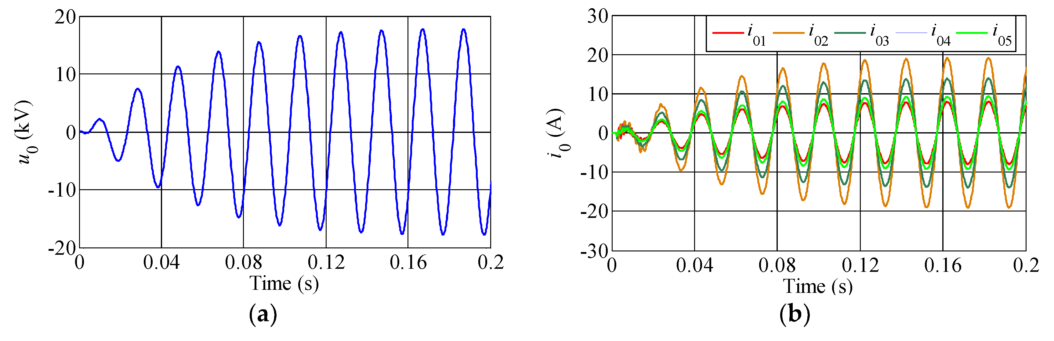
4.2.2. Simulation Verification in Under-Damping State
A single-phase-to-ground fault through 1000Ω transition resistance with a voltage inception angle 60° is conducted in K4. Figure 6 records the sampled bus zero-sequence voltage and zero-sequence currents of all the feeders. As seen from Figure 6, it is evident that the transient process is under-damping state because of oscillatory attenuation phenomenon. Similarly, the transient components of them need to be extracted by means of fault components and post-fault steady-state components. The extraction results are shown in Figure 7.
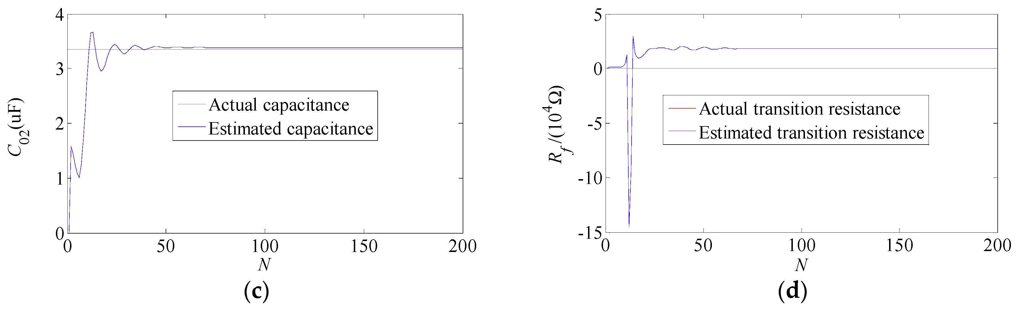
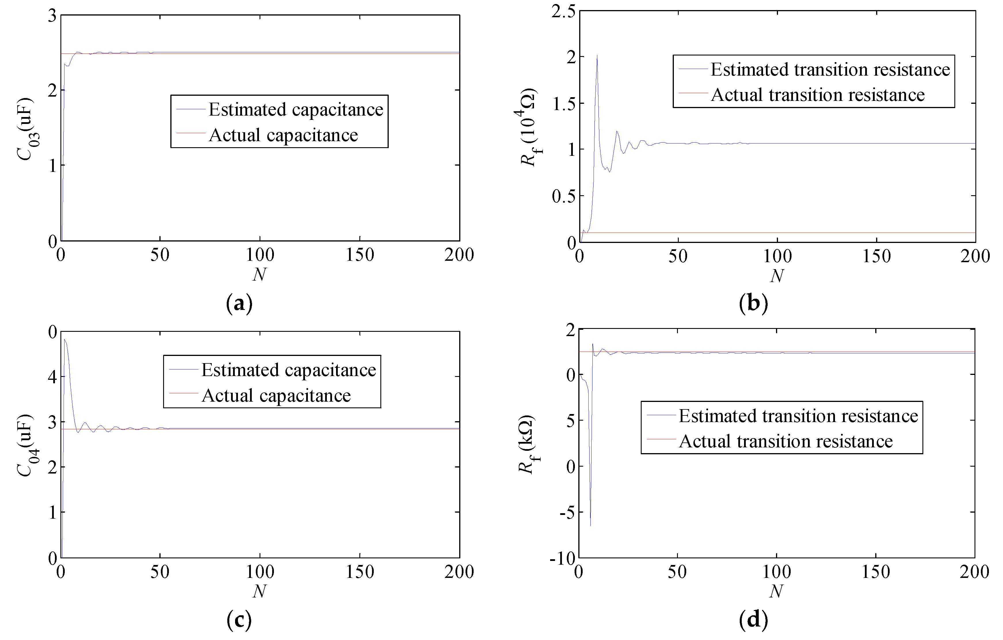
As shown in Figure 8, in the case of under-damping state, the estimated capacitances of feeder 3 and feeder 4 are approximate to actual capacitances, respectively. However, the estimated resistance of feeder 3 is much greater than the set threshold 5000 Ω, while the estimated resistance of feeder 4, which is close to the actual value and is far less than the set threshold. In consequence, feeder 3 is regarded as a healthy feeder and feeder 4 is identified as faulty feeder accurately and reliably.
4.2.3. Simulation Verification under Different Fault Conditions
To verify the performance of the proposed method on different fault conditions, multiple simulations are carried out considering different fault points, different transition resistances, and different voltage inception angles. The simulation results are presented in Table 1. Since the estimated capacitances are not required for the identification of faulty feeder, only the estimated transition resistances of all feeders are shown in the table.
It is found from Table 1 that the estimated transition resistances of faulty feeders are almost equal to actual transition resistances and far less than set threshold, while the estimated transition resistances of healthy feeders are much larger than actual values as well as set threshold under different fault conditions. Accordingly, it is proved that the proposed method has good adaptability for faulty feeder identification of the single-phase HIF in RGDS.
4.2.4. Comparison with Other Methods
In order to validate the superiority of proposed method for the single-phase HIF in RDGS, a comparison between the proposed method and the fifth harmonic method (FHM) and wavelet packet energy method (WPEM), which are widely used in practical application is conducted. For the FHM, the feeder which has the biggest amplitude of fifth harmonic is regard as faulty feeder. For WPEM, the feeder, which has maximum energy in feature band that has the most concentrated fault component, is identified as the faulty feeder [16].
A single-phase HIF through transition resistance 1000 Ω with a voltage inception angle 60° is imposed on feeder 4. The amplitude of fifth harmonic is extracted by full wave Fourier transform. The energy is obtained by calculating the square of wavelet packet coefficients in the feature band. In the wavelet packet transform, db 5 wavelet is chosen and the decomposition is 5. Sampling data of two fundamental frequency cycles is adopt. The comparison results between the proposed method and FHM and WPEM are shown in Table 2. As shown in the table, it is evident that the FHM and WPEM developed the misjudgment in the case of the HIF, while the proposed method identified the faulty feeder correctly. Therefore, it is conclude that the proposed method has a better performance for the faulty feeder identification of the single-phase HIF in RDGS.
4.3. RTDS Based Experiment Results
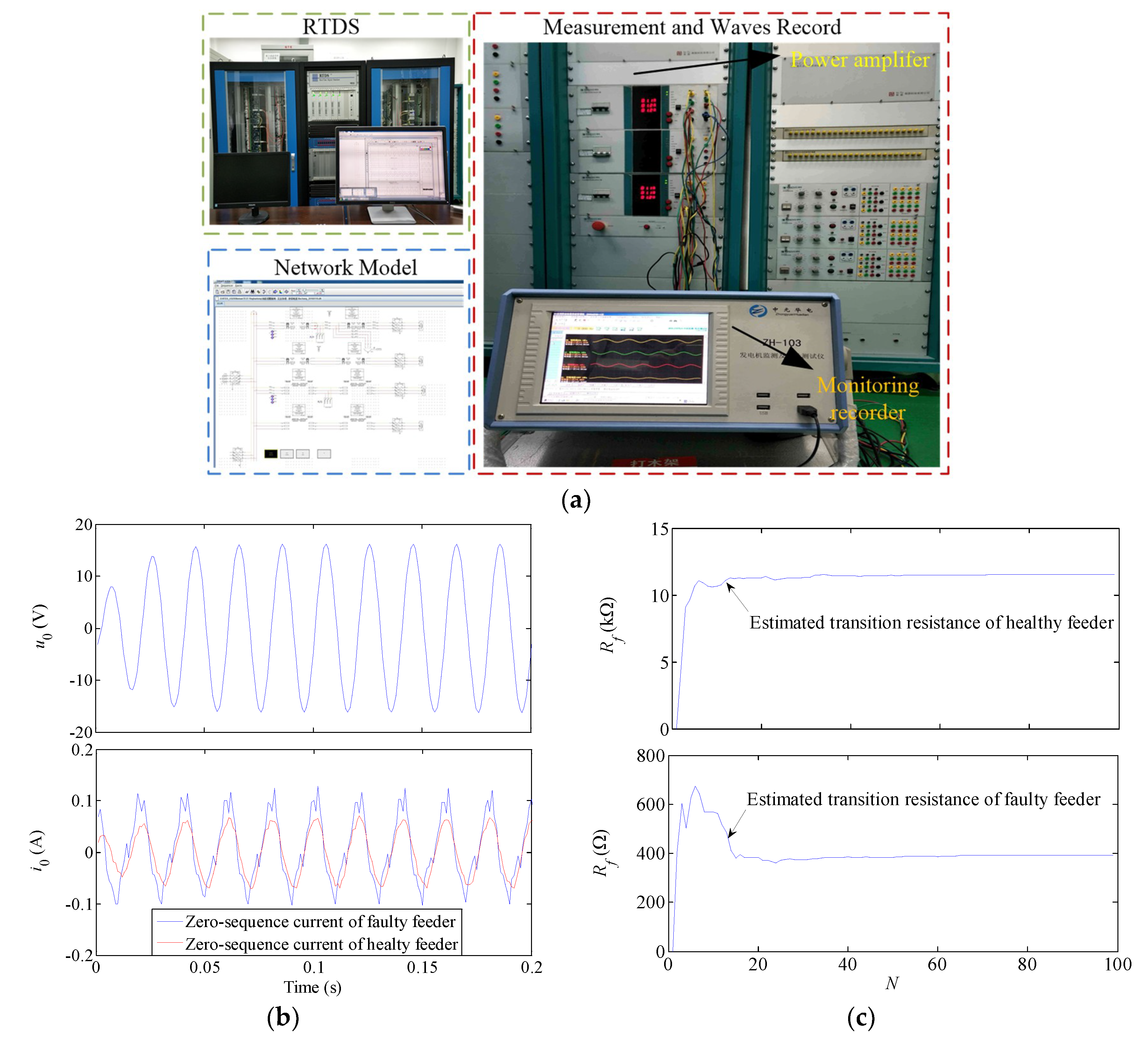
In order to evaluate further the performance of the proposed method, the RTDS based experiment platform is set up and is shown as Figure 9a. The instrument which is developed and manufactured by Manitoba RTDS company, Canada, is used to study electromagnetic transient phenomena in power systems. Firstly, the RGDS model in reference to a practical network in Changsha city of Hunan province of China is established. Then, a HIF is imposed in a feeder and the simulation based on RTDS is tested. After that, bus zero-sequence voltage and zero-sequence currents of two feeders which include a faulty feeder and a healthy feeder are exported by power amplifier. In order to make the experiment results compatible with the real world, the exported bus zero-sequence voltage and feeders’ zero-sequence currents are measured and recorded by a clamp type ammeter and a wave recorded equipment, respectively, and the recorded waveforms, which are close to field measured waveforms are shown in Figure 9b.
As seen from simulation results in Figure 9c, the estimated transition resistance of the faulty feeder is about 400 Ω, which is far less than set threshold. However, the estimated transition resistance of healthy feeder is about are 12 kΩ that is much larger than the set threshold. Hence, it is confirmed that the proposed method has a strong adaptability for faulty feeder identification of the single-phase HIF in RGDS.
5. Conclusions
After a single-phase HIF takes place in RGDS, fault current is very low and the fault cannot be detected by traditional over-current relays, for improvement, a faulty feeder identification method for HIF is proposed.
During the single-phase HIF, the transient process of the system will present an over-damping state and under-damping state under different transition resistance. For both states, the transient zero-sequence current of the healthy feeder is proportional to bus transient zero-sequence voltage derivative, and the proportional coefficient is feeder own capacitance; while transient zero-sequence current of faulty feeder is linear relationship between bus transient zero-sequence voltage and the bus transient zero-sequence voltage derivative, and the coefficients are the reciprocal of transition resistance and feeder own capacitance value, respectively. To identify faulty feeder, the transition resistance of each feeder is estimated by the least squares algorithm. For healthy feeder, the estimated transition resistance is a large value and is much larger than set threshold. However, for faulty feeder, the estimated transition resistance is approximately equal to the actual fault resistance value and is far less than set threshold. Thus, faulty feeder can be detected.
By contrast, it is discovered that the proposed method has a superior performance in the case of single-phase HIFs. Extensive simulations and RTDS experiment tests show that the proposed method is able to identify faulty feeder accurately and effectively, and it is suitable for single-phase HIFs in RGDS.
Author Contributions
T.T. is the main author of this work, which has been counseled by C.H., Z.X.L., and X.G.Y. All authors have contributed to extensive revisions of the text.
Funding
This work was supported by National Natural Science Foundations of China (51577013), (51677060), (51877011).
Conflicts of Interest
The authors declare no conflict of interest.
References
- Dong, X.; Shi, S. Identifying single-phase-to-ground fault feeder in neutral noneffectively grounded distribution system using wavelet transform. IEEE Trans. Power Deliv. 2008, 23, 1829–1837. [Google Scholar] [CrossRef]
- Zeng, X.; Li, K.K.; Chan, W.L.; Su, S.; Wang, Y. Ground-fault feeder detection with fault-current and fault-resistance measurement in mine power systems. IEEE Trans. Ind. Appl. 2008, 44, 424–429. [Google Scholar] [CrossRef]
- Wang, X.; Song, G.; Chang, Z.; Luo, J.; Gao, J.; Wei, X.; Wei, Y. Faulty feeder detection based on mixed atom dictionary and energy spectrum energy for distribution network. IET Gener. Transm. Distrib. 2017, 12, 596–606. [Google Scholar] [CrossRef]
- Zamora, I.; Mazón, A.J.; Sagastabeitia, K.J.; Zamora, J.J. New method for detecting low current faults in electrical distribution systems. IEEE Trans. Power Deliv. 2007, 22, 2072–2079. [Google Scholar] [CrossRef]
- Lin, X.; Sun, J.; Kursan, I.; Zhao, F.; Li, Z.; Li, X.; Yang, D. Zero-sequence compensated admittance based faulty feeder selection algorithm used for distribution network with neutral grounding through Peterson-coil. Int. J. Electr. Power Energy Syst. 2017, 32, 23–32. [Google Scholar] [CrossRef]
- Personal, E.; García, A.; Parejo, A.; Larios, D.F.; Biscarri, F.; León, C. A comparison for impedance-based fault location methods for power underground distribution systems. Energies 2016, 9, 1022. [Google Scholar] [CrossRef]
- Sang, Z.; Zhang, H.; Pan, Z.; Tian, Z. Protection for single phase to earth fault line selection for ungrounded power system by injecting signal. Autom. Electr. Power Syst. 1996, 20, 11–12. [Google Scholar]
- Huang, C.; Tang, T.; Jiang, Y.; Hua, L.; Hong, C. Faulty feeder detection by adjusting the compensation degree of arc-suppression coil for distribution network. IET Gener. Transm. Distrib. 2018, 12, 807–814. [Google Scholar] [CrossRef]
- Lin, X.; Huang, J.; Ke, S. Faulty feeder detection and fault self-extinguishing by adaptive Petersen coil control. IEEE Trans. Power Deliv. 2011, 26, 1290–1291. [Google Scholar] [CrossRef]
- Zhang, Z.; Liu, X.; Piao, Z. Fault line detection in neutral point ineffectively grounding power system based on phase-locked loop. IET Gener. Transm. Distrib. 2014, 8, 273–280. [Google Scholar]
- Li, Y.; Meng, X.; Song, X. Application of signal processing and analysis in detecting single line-to-ground (SLG) fault location in high-impedance grounded distribution network. IET Gener. Transm. Distrib. 2016, 18, 382–389. [Google Scholar] [CrossRef]
- Cui, T.; Dong, X.; Bo, Z.; Juszczyk, A. Hilbert-transform-based transient/intermittent earth fault detection in noneffectively grounded distribution systems. IEEE Trans. Power Deliv. 2011, 26, 143–151. [Google Scholar] [CrossRef]
- Michalik, M.; Rebizant, W.; Lukowicz, M.; Lee, S.-J.; Kang, S.-H. High-impedance fault detection in distribution networks with use of wavelet-based algorithm. IEEE Trans. Power Deliv. 2006, 21, 1793–1802. [Google Scholar]
- Sarlak, M.; Shahrtash, S.M. High impedance fault detection using combination of multi-layer perceptron neural networks based on multi-resolution morphological gradient features of current waveform. IET Gener. Transm. Distrib. 2011, 5, 588–595. [Google Scholar] [CrossRef]
- Etemadi, A.H.; Pasand, M.S. High-impedance fault detection using multi-resolution signal decomposition and adaptive neutral fuzzy inference system. IET Gener. Transm. Distrib. 2008, 2, 110–118. [Google Scholar] [CrossRef]
- Wang, Y.; Huang, Y.; Zeng, X.; Wei, G.; Zhou, J.; Fang, T.; Chen, H. Faulty feeder detection of single phase-earth fault using grey relation degree in resonant grounding system. IEEE Trans. Power Deliv. 2017, 32, 55–61. [Google Scholar] [CrossRef]
- Suresh, G.; Sukumar, M.B. Detection of high impedance fault in power distribution systems using mathematical morphology. IEEE Trans. Power Syst. 2013, 28, 1226–1234. [Google Scholar]
- Jota, F.G.; Jota, P.R.S. High-impedance fault identification using a fuzzy reasoning system. IET Gener. Transm. Distrib. 1998, 145, 656–661. [Google Scholar] [CrossRef]
- Ghaderi, A.; Mohammadpour, H.A.; Ginn, H.L.; Shin, Y. High-impedance fault detection in the distribution network using the time-frequency-based algorithm. IEEE Trans. Power Deliv. 2015, 30, 1260–1268. [Google Scholar] [CrossRef]
- Henriksen, T. Faulty feeder identification in high impedance grounded network using charge-voltage relationship. Electr. Power Syst. Res. 2011, 81, 1832–1839. [Google Scholar] [CrossRef]
- Li, T.Y.; Xue, Y.D.; Xu, B.Y. High-impedance fault detection technology based on transient information in a resonant grounding system. CIRED Open Access Proc. J. 2017, 2017, 1176–1179. [Google Scholar] [CrossRef]
Figure 1.
Equivalent zero-sequence network for single-phase high impedance faults (HIF) in resonant grounding distribution system (RGDS).
Figure 1.
Equivalent zero-sequence network for single-phase high impedance faults (HIF) in resonant grounding distribution system (RGDS).

Figure 2.
Simulation model for the single-phase HIF in RGDS.
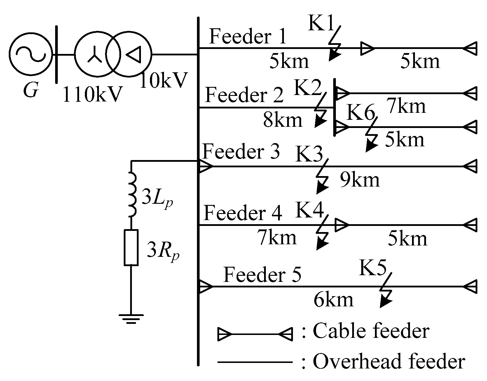
Figure 3.
Bus zero-sequence voltage and zero-sequence current of each feeder for a single-phase HIF in K1 point. (a) Bus zero-sequence voltage; and (b) Feeders’ zero-sequence currents.
Figure 3.
Bus zero-sequence voltage and zero-sequence current of each feeder for a single-phase HIF in K1 point. (a) Bus zero-sequence voltage; and (b) Feeders’ zero-sequence currents.

Figure 4.
Transient components of bus zero-sequence voltage and feeders’ zero-sequence currents for a single-phase HIF in K1 point. (a) Transient component of bus zero-sequence voltage; and (b) Transient components of feeders’ zero-sequence currents.
Figure 4.
Transient components of bus zero-sequence voltage and feeders’ zero-sequence currents for a single-phase HIF in K1 point. (a) Transient component of bus zero-sequence voltage; and (b) Transient components of feeders’ zero-sequence currents.

Figure 5.
Estimated capacitances and transition resistances of feeder 1 and feeder 2 for a single-phase HIF in K1 point. (a) Estimated capacitance of feeder 1; (b) Estimated transition resistance of feeder 1; (c) Estimated capacitance of feeder 2; and (d) Estimated transition resistance of feeder 2.
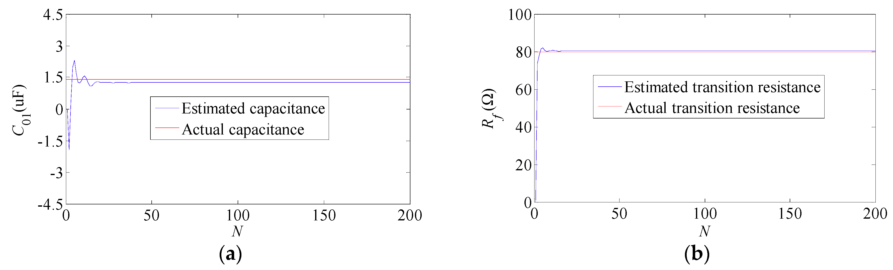

Figure 6.
Bus zero-sequence voltage and zero-sequence current of each feeder for a single-phase HIF in K4 point. (a) Bus zero-sequence voltage; and (b) Feeders’ zero-sequence currents.
Figure 6.
Bus zero-sequence voltage and zero-sequence current of each feeder for a single-phase HIF in K4 point. (a) Bus zero-sequence voltage; and (b) Feeders’ zero-sequence currents.

Figure 7.
Transient components of bus zero-sequence voltage and feeders’ zero-sequence currents for a single-phase HIF in K4 point. (a) Transient component of bus zero-sequence voltage; (b) Transient components of feeders’ zero-sequence currents.
Figure 7.
Transient components of bus zero-sequence voltage and feeders’ zero-sequence currents for a single-phase HIF in K4 point. (a) Transient component of bus zero-sequence voltage; (b) Transient components of feeders’ zero-sequence currents.

Figure 8.
Estimated capacitances and transition resistances of feeder 1 and feeder 2 for a single-phase HIF in K4 point. (a) Estimated capacitance of feeder 3; (b) Estimated transition resistance of feeder 3; (c) Estimated capacitance of feeder 4; and (d) Estimated transition resistance of feeder 4.

Figure 9.
Experiment platform based on RTDS and simulation results of the proposed method. (a) Experiment platform based on RTDS; (b) Bus zero-sequence voltage and zero-sequence currents of a faulty feeder and a healthy feeder; and (c) Estimated transition resistances for the faulty feeder and healthy feeder.

Table 1.
Simulation results of the proposed method for faulty feeder identification under different fault conditions.
Table 1.
Simulation results of the proposed method for faulty feeder identification under different fault conditions.
| Fault Points | Rf (Ω)/θ (°) | Feeder 1 Rf (kΩ) | Feeder 2 Rf (kΩ) | Feeder 3 Rf (kΩ) | Feeder 4 Rf (kΩ) | Feeder 5 Rf (kΩ) | Rset | Identifing Results |
|---|---|---|---|---|---|---|---|---|
| K1 | 2000/90 | 2.0840 | 8.1000 | 10.535 | 20.674 | 17.339 | 5 kΩ | Feeder 1 |
| 900/0 | 0.8560 | 8.7230 | 10.917 | 18.687 | 17.856 | |||
| K2 | 1200/90 | 20.745 | 1.1610 | 10.492 | 20.477 | 17.257 | Feeder 2 | |
| 150/45 | 23.304 | 0.1450 | 10.099 | 27.389 | 18.840 | |||
| K3 | 1500/100 | 20.804 | 8.0970 | 1.4950 | 20.534 | 17.283 | Feeder 3 | |
| 200/135 | 14.619 | 15.681 | 0.2010 | 15.787 | 17.316 | |||
| K4 | 1800/75 | 21.156 | 8.1980 | 10.716 | 1.6030 | 17.625 | Feeder 4 | |
| 500/60 | 21.138 | 8.5720 | 10.583 | 0.4850 | 17.401 | |||
| K5 | 1000/150 | 21.112 | 8.2860 | 10.658 | 17.525 | 0.9440 | Feeder 5 | |
| 350/30 | 23.024 | 8.8770 | 10.555 | 22.297 | 0.3460 | |||
| K6 | 100/45 | 23.372 | 0.1010 | 11.006 | 25.875 | 17.900 | Feeder 2 |
The bold values indicate the estimated transition resistances of faulty feeders.
Table 2.
Comparison results between the proposed method (PM) and FHM and wavelet packet energy method(WPEM).
Table 2.
Comparison results between the proposed method (PM) and FHM and wavelet packet energy method(WPEM).
| Methods | Extracted Characteristic | Faulty Feeder | Result | ||||
|---|---|---|---|---|---|---|---|
| PM | 21.11 | 8.284 | 10.66 | 0.968 | 17.53 | feeder 4 | right |
| FHM | 0.034 | 0.070 | 0.061 | 0.062 | 0.042 | feeder 2 | wrong |
| WPEM | 1368 | 7898 | 4187 | 6402 | 1862 | feeder 2 | wrong |
The PM indicates the proposed method; The bold values indicate characteristic values of faulty feeder identified.
© 2019 by the authors. Licensee MDPI, Basel, Switzerland. This article is an open access article distributed under the terms and conditions of the Creative Commons Attribution (CC BY) license (http://creativecommons.org/licenses/by/4.0/).
Share and Cite
MDPI and ACS Style
Tang, T.; Huang, C.; Li, Z.; Yuan, X. Identifying Faulty Feeder for Single-Phase High Impedance Fault in Resonant Grounding Distribution System. Energies 2019, 12, 598. https://doi.org/10.3390/en12040598
AMA Style
Tang T, Huang C, Li Z, Yuan X. Identifying Faulty Feeder for Single-Phase High Impedance Fault in Resonant Grounding Distribution System. Energies. 2019; 12(4):598. https://doi.org/10.3390/en12040598
Chicago/Turabian StyleTang, Tao, Chun Huang, Zhenxing Li, and Xiuguang Yuan. 2019. "Identifying Faulty Feeder for Single-Phase High Impedance Fault in Resonant Grounding Distribution System" Energies 12, no. 4: 598. https://doi.org/10.3390/en12040598
Note that from the first issue of 2016, this journal uses article numbers instead of page numbers. See further details here.