Fault Tolerant Control of DFIG-Based Wind Energy Conversion System Using Augmented Observer

Abstract

An augmented sliding mode observer is proposed to solve the actuator fault of an uncertain wind energy conversion system (WECS), which can estimate the system state and reconstruct the actuator faults. Firstly, the mathematical model of the WECS is established, and the non-linear term in the state equation is separated as the uncertain part of the system. Then, the states of the system are augmented, and the actuator fault is considered as part of the augmented state. The augmented sliding mode observer is designed to estimate the system state and actuator fault. A robust fault-tolerant controller is designed to ensure the reliable input of the WECS, maintain the stability of the fault system and maximize the acquisition of wind energy. The numerical simulation results verify the effectiveness of the control strategy.

1. Introduction

Wind power generation is the most mature and promising form of new energy generation [1]. The wind energy conversion system (WECS) is an important part of the wind power generation system. It is generally located in the complex terrain and harsh climate environment such as mountain islands. The WECS is prone to frequent faults, seriously affecting the performance of the wind power system, and even causing paralysis of the system, resulting in incalculable losses. Therefore, it is of great practical significance to improve the reliability and security of the WECS [2,3].

There are many control methods currently applied to fault-tolerant control of the WECS. Observer-based fault diagnosis and fault-tolerant control have received extensive attention [4]. Reference [5] estimates the fault of fan pitch actuator by combining a disturbance compensation device with a controller, then modifies the pitch control law appropriately to achieve fault tolerant control comparable to that without fault. An adaptive active fault-tolerant fuzzy controller was designed by using multi-observer switching control strategy to ensure the stability of the WECS, considering the interaction of parameter uncertainties and sensor faults in [6]. Reference [7] proposed a fuzzy reference adaptive control, which adapts the parameters to achieve fault-tolerant control in the case of uncertain system potential faults, so as to adjust the generator torque value. In [8], the convex decomposition theory is used to transform the non-linear model of the fan into the linear model, and the state feedback method is used to obtain the fault-tolerant control of the virtual actuator. In [9], an adaptive fault observer is constructed to diagnose the transmission faults of the WECS and to implement fault-tolerant control. Due to the strict design conditions of traditional observers, the scope of application is limited. High-order sliding mode control strategy is also widely used [10,11,12,13]. The high-order sliding mode based on DFIG (doubly fed induction generator) used in [10] as an improved scheme to deal with the classical sliding mode chattering problem, which is robust to external disturbances. Reference [11] adopted maximum power point tracking, optimal fault adaptive tracking and adaptive robust non-linear control combined with high-order sliding mode to control open-circuit fault of generator. Reference [12] presented a second-order sliding mode control based on DFIG wind power generation system, and controls the wind power generation system according to the reference value given by Maximum Power Point Tracking, so as to obtain the maximum power extraction.

A new state variable is composed of input and state variables to form a singular system, which provides an idea for the method of unknown input observer for nonlinear systems [14]. In [15], the output noise and the state variables of the original system are combined into a new generalized system, and a generalized sliding mode observer is designed for the system. Then, H_∞ is used to guarantee the robustness and estimate the output noise. An extended sliding mode observer is designed to estimate external disturbances and system states simultaneously, which widens the application scope of fault diagnosis observer in [16]. Reference [17] reduced the influence of process disturbance by constructing augmented state vector composed of system states and related faults, and estimating system states and related faults. In [18], the discrete linear model is used to design the sliding mode controller. The stability and robustness of the nonlinear system are improved by adding discrete operators to improve the discrete sliding mode controller. A new design method of augmented fault diagnosis observer is proposed in [19], which separates the observer from the output feedback fault-tolerant device and simplifies the design process. In [20], the augmented system, unknown input fuzzy observer and linear matrix inequality are combined to design robust fault estimation and fault tolerance control approach for T-S fuzzy systems, which are applied to 4.8-MW wind turbines system.

In practice, the phenomena of abrupt disturbance, sensor faults and actuator faults are very common, and further studies are urgently needed. From the above research, it can be seen that for wind power generation system, fault reconfiguration and fault tolerance of design robust sliding mode observer can be achieved by enlarging the system, which reduces the knowledge and experience requirements of the system. The design process is simple and easy to implement, and improves the robustness of the system.

In this paper, an augmented sliding mode observer is proposed to solve the actuator fault of uncertain WECS. By dividing the non-linear term into a constant matrix and an uncertainty matrix, and augmenting the system state, the actuator fault is augmented as a part of the system state, and an augmented sliding mode observer is constructed. The equivalent output control method is used to reconstruct the fault without affecting the state estimation. The active fault-tolerant controller is designed to ensure the reliable input of the WECS. Finally, the proposed method is validated on the wind turbine model.

2. Mathematical Modeling of Double-fed WECS

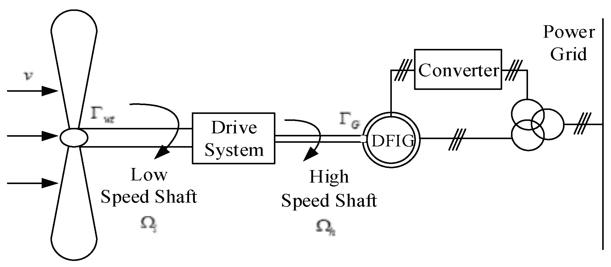
The WECS is mainly composed of wind turbine, transmission system, generator, AC-DC converter, power grid and so on. Wind turbines convert the captured wind energy into mechanical energy, drive the doubly-fed induction motor to rotate through the transmission link, and transmit the generated energy to the power grid [21]. The DFIG-based WECS is shown in Figure 1.

According to Betz’ Law, assuming that the wind turbine is in an ideal state, the mechanical power obtained by the wind turbine is as follows [22]:

$$P_{wt}=0.5\pi R^2\rho v^3{C}_p(\lambda ,\beta )$$

(1)

where, P_wt is the mechanical power captured by the wind turbine, ρ is the air density, ν is the wind speed, R is the fan blade length; C_p(λ,β) is the wind energy conversion coefficient, which is a function of tip velocity ratio λ and pitch angle β. Λ is the ratio of tip speed to wind speed, that is λ = Ω_l(R/ν), where Ω_l is the angular velocity of the wind turbine rotor, that is, the low speed axis.

Equation (1) shows that when the wind speed is constant, the mechanical power captured by the wind turbine is only related to C_p(λ,β). If the pitch angle β of the wind turbine remains unchanged, the wind energy conversion coefficient C_p is only related to the tip speed ratio λ. For different types of wind turbines, there is an unique optimal tip speed ratio λ to ensure the best wind energy conversion coefficient C_p and achieve maximum wind energy capture.

The wind torque generated by the wind wheel is as follows:

$${\mathsf{\Gamma }}_{wt}=\frac{P_{wt}}{{\mathsf{\Omega }}_l}=0.5\pi \rho v^2{R}^3{C}_{\mathsf{\Gamma }}(\lambda ,\beta )$$

(2)

where, C_Γ(λ,β) = C_p(λ,β)/λ is the torque coefficient.

The transmission system of the WECS is mainly composed of the wind turbine rotor, low speed shaft, variable speed gear, high speed shaft and generator rotor. The mechanical energy from the fan drives the low-speed shaft to rotate, and electromagnetic torque is produced. Through the gear box transformation, the lower speed of the blade is increased to a higher speed, which is transmitted to the generator rotor to drive the DFIG to rotate, and the electric energy is output to the power grid. For simplicity, rigid models are generally used for the connection between high-speed and low-speed axles. The dynamic equations are as follows:

$$J_h\frac{d{\mathsf{\Omega }}_h}{d_t}=\frac{\eta }{i_0}{\mathsf{\Gamma }}_{wt}-{\mathsf{\Gamma }}_G$$

(3)

$$J_t\frac{d{\mathsf{\Omega }}_l}{d_t}={\mathsf{\Gamma }}_{wt}-\frac{i_0}{\eta }{\mathsf{\Gamma }}_G$$

(4)

where, Ω_h is the rotor speed (high speed shaft) of the generator, that is Ω_l = i_o × Ω, i_o is the gear transmission speed ratio. Γ_G is the electromagnetic torque of the generator, η is the transmission efficiency, J_h is the inertia of the high-speed axis, J_t is the inertia of the low-speed axis.

Based on the power coefficient and the optimal tip speed ratio λ, considering that the generator is in an ideal state, the state equation of the WECS [23] is modeled as follows:

$$\{\begin{array}{l}{\dot{\mathsf{\Omega }}}_h(t)=\frac{{\mathsf{\Gamma }}_{wt}(i_0\cdot {\mathsf{\Omega }}_h,v)}{i_0\cdot J_t}-\frac{{\mathsf{\Gamma }}_G}{J_t}\\ {\dot{\mathsf{\Gamma }}}_G(t)=-\frac{{\mathsf{\Gamma }}_G}{T_g}+\frac{{\mathsf{\Gamma }}_{ref}^{\ast }}{T_g}\end{array}$$

(5)

where, ${\mathsf{\Gamma }}_{ref}^{\ast }$ is the reference value of the electromagnetic torque of the generator and T_G is the electromagnetic time constant. Taking Ω_h and Γ_G as state vectors, the state equation of the WECS is obtained as shown in (6):

$$\{\begin{array}{l}\dot{x}(t)=A^{\prime }x(t)+Bu(t)\\ y(t)=Cx(t)\end{array}$$

(6)

where, $\dot{x}$(t) = [Ω_h Γ_G]^T, u(t) = ${\mathsf{\Gamma }}_{ref}^{\ast }$, $A^{\prime }=\left[\begin{array}{cc}\frac{{\mathsf{\Gamma }}_{wt}(i_0{\mathsf{\Omega }}_h,\nu }{i_o{J}_t{\mathsf{\Omega }}_h}& -\frac{1}{J_t}\\ 0& -\frac{1}{T_G}\end{array}\right]$, $B=\left[\begin{array}{c}0\\ \frac{1}{T_G}\end{array}\right]$, $C=\left[\begin{array}{cc}1& 0\\ 0& 1\end{array}\right]$, x(t) is the state vector, u(t) is the input vector, y(t) is the output vector.

3. Actuator Fault Model of the WECS

Actuator faults are generally caused by wear and tear of gears in gearboxes, wear and deformation of bearing tooth surfaces, and are affected by some uncertainties of the system. Considering these faults of the WECS [24], the system can be described as:

$$\{\begin{array}{l}\dot{x}(t)=A^{\prime }x(t)+Bu(t)+D{f}_a(t)\\ y(t)=Cx(t)\end{array}$$

(7)

where, x ∈ Rⁿ is the state variable, u ∈ R^m is the input vector and y ∈ R^p is the measurable output vector, f_a ∈ R^q represents an unknown but bounded actuator fault of the system, A′ ∈ R^m×n, B ∈ R^n×m, C ∈ R^p×n, D ∈ R^n×q. The system matrix A′ is split into the form of the sum of an uncertain matrix and a constant matrix, that is A′ = ΔA, $A=\left[\begin{array}{cc}0& -\frac{1}{J_t}\\ 0& -\frac{1}{T_G}\end{array}\right]$, $\Delta A=\left[\begin{array}{cc}\frac{{\mathsf{\Gamma }}_{wt}\left(i_0{\mathsf{\Omega }}_h,\nu \right)}{i_o{J}_{ty}{\mathsf{\Omega }}_h}& 0\\ 0& 0\end{array}\right]$ where $\Delta Ax=Md\left(x,u,t\right)={\left[\frac{{\mathsf{\Gamma }}_{wt}\left(i_o{\mathsf{\Omega }}_h,\nu \right)}{i_o{J}_t} 0\right]}^T$, where d(x,u,t) ∈ R^h, M ∈ R^n×h. d(x,u,t) is regarded as an unknown input disturbance of the system, and Equation (7) can be converted into (8):

$$\{\begin{array}{l}\dot{x}(t)=Ax(t)+Bu(t)+D{f}_a(t)+Md(x,u,t)\\ y(t)=Cx(t)\end{array}$$

(8)

We assume that the system (8) satisfies the following conditions:

Assumption 1. The unknown input disturbance d(x,u,t) and the actuator fault f_a satisfy $\Vert d\left(x,u,t\right)\Vert \le d_0$ and $\Vert f_a\Vert \le {\alpha }_0$, where d₀ > 0, α₀ > 0 is a known constant.

Assumption 2. The system satisfies that (A,B) is stable and (A,C) is observable.

Assumption 3. There is a positive scalar δ, which satisfies $rank\left[\begin{array}{cc}\delta I_n+A& D\\ C& 0\end{array}\right]=n+q$.

The actuator fault is considered as part of augmented state to build the augmented system. Definition: $\overline{x}\left(t\right)=\left[\begin{array}{c}x\left(t\right)\\ f_a\left(t\right)\end{array}\right]$. The following augmented system (9) can be obtained:

$$\begin{gathered} \underset{\overline{E}}{\underbrace{\left[\begin{array}{cc}{I}_n& {\delta }^{-1}D\\ 0& I_q\end{array}\right]}}\underset{\dot{\overline{x}}(t)}{\underbrace{\left[\begin{array}{c}\dot{x}(t)\\ {\dot{f}}_a(t)\end{array}\right]}}=\underset{\overline{A}}{\underbrace{\left[\begin{array}{cc}A& 0\\ 0& -\delta I_q\end{array}\right]}}\underset{\overline{x}(t)}{\underbrace{\left[\begin{array}{c}x(t)\\ f_a(t)\end{array}\right]}}+\underset{\overline{B}}{\underbrace{\left[\begin{array}{c}B\\ 0_{q\times m}\end{array}\right]}}u(t)+\underset{\overline{D}}{\underbrace{\left[\begin{array}{cc}{\delta }^{-1}D& M\\ I_q& 0_{q\times h}\end{array}\right]}}\underset{\overline{f}(t)}{\underbrace{\left[\begin{array}{c}\delta f_a(t)+{\dot{f}}_a(t)\\ d(x,u,t)\end{array}\right]}} \\ y(t)=\underset{\overline{C}}{\underbrace{\left[\begin{array}{cc}C& 0_{p\times q}\end{array}\right]}}\underset{\overline{x}(t)}{\underbrace{\left[\begin{array}{c}x(t)\\ f_a(t)\end{array}\right]}} \end{gathered}$$

(9)

Then Equation (9) is transformed into Equation (10):

$$\{\begin{array}{l}\overline{E}\dot{\overline{x}}(t)=\overline{A}\overline{x}(t)+\overline{B}u(t)+\overline{D}\overline{f}(t)\\ y(t)=\overline{C}\overline{x}(t)\end{array}$$

(10)

where, $\overline{E}\in R^{n+q}$.

4. Design of the Augmented Sliding Mode Observer

When assumptions 1-3 are satisfied, an augmented sliding mode observer is designed to effectively suppress the effect of actuator faults, uncertainties and external disturbances. The state estimation of augmented system is realized, and the dynamic equations of augmented error system and sliding mode state are obtained. The augmented sliding mode observer (11) is designed as follows:

$$\{\begin{array}{l}\overline{E}\dot{\widehat{\overline{x}}}=(\overline{A}-L_p\overline{C})\widehat{\overline{x}}(t)+\overline{B}u(t)+L_{p}y(t)+L_s{u}_s(t)\\ \widehat{y}(t)=\overline{C}\widehat{\overline{x}}(t)\end{array}$$

(11)

where, L_p ∈ R^(n+q)×p is the undetermined gain matrix of the sliding mode observer, and L_s ∈ R^(n+q)×(q+h) is the sliding mode gain matrix of the sliding mode observer. u_s ∈ R^q+h is a non-continuous sliding mode input term, which eliminates the effect of system actuator faults and uncertainties. It is defined as Equation (12):

$$u_s=\{\begin{array}{l}-\rho \frac{H{e}_y}{\Vert H{e}_y\Vert }, e_y\ne 0\\ 0 , e_y=0\end{array}$$

(12)

where, $\rho =\delta {\alpha }_0+d_0+\gamma$, and γ > 0 is any small positive parameter.

For system (11), the sliding mode gain matrix $L_s=\overline{D}$ is designed. The state error of the system is defined as $e\left(t\right)=\widehat{x}\left(t\right)-x\left(t\right)$, the output estimation error is $e_y=\widehat{y}\left(t\right)-y\left(t\right)$, and the Lyapunov matrix P satisfies ${\overline{D}}^T{\left({\overline{E}}^{-1}\right)}^{T}P=HC$, where, H ∈ R^(q+h)×p is a parameter matrix determined by the Lyapunov matrix P.

When Equation (11) is subtracted from Equation (10), the deviation system (13) can be obtained:

$$\overline{E}\dot{e}(t)=(\overline{A}-L_p\overline{C})e(t)+L_s{u}_s-\overline{D}\overline{f}(t)$$

(13)

Since $\overline{E}$ is the nonsingular matrix, there must be the matrix ${\overline{E}}^{-1}$. The error dynamic model of augmented system (14) can be derived by the left multiplication of Equation (10):

$$\dot{e}(t)={\overline{E}}^{-1}(\overline{A}-L_p\overline{C})e(t)+{\overline{E}}^{-1}{L}_s{u}_s-{\overline{E}}^{-1}\overline{D}\overline{f}(t)$$

(14)

Lemma 1: There exists a proportional gain matrix $L_p=S{X}^{-1}{\overline{C}}^T$ so that C satisfies the

Roulth-Holwitz criterion ${\overline{E}}^{-1}\left(\overline{A}-L_p\overline{C}\right)$. X¹ satisfies the Lyapunov equation $-{\left(\mu I+{\overline{E}}^{-1}\overline{A}\right)}^{T}X-X\left(\mu I+{\overline{E}}^{-1}\overline{A}\right)=-{\overline{C}}^T\overline{C}$ and μ > 0, which satisfies $\mathrm{R}e\left[{\lambda }_i\left({\overline{E}}^{-1}\overline{A}\right)\right]>-\mu$.

The proof is as follows:

Since $\mathrm{R}e\left[{\lambda }_i\left({\overline{E}}^{-1}\overline{A}\right)\right]>-\mu , \forall i\in \left\{1,2,\dots ,n+p\right\}$ is equivalent to $\mathrm{R}e\left[{\lambda }_i\left(-\left(\mu I+{\overline{E}}^{-1}\overline{A}\right)\right)\right]<0,\forall i\in \left\{1,2,\dots ,n+p\right\}$, it can be concluded that for $\forall s\in R^{+}$, Equations (15) and (16) are valid, as follows:

$$rank\left[\begin{array}{c}s{I}_{n+p}-{\overline{E}}^{-1}\overline{A}\\ \overline{C}\end{array}\right]=rank\left[\begin{array}{cc}{\overline{E}}^{-1}& 0\\ 0& I_p\end{array}\right]\left[\begin{array}{c}s\overline{E}-\overline{A}\\ \overline{C}\end{array}\right]=rank\left[\begin{array}{c}s\overline{E}-\overline{A}\\ \overline{C}\end{array}\right]$$

(15)

$$rank\left[s\overline{E}-\overline{A}\right]=rank\left[\begin{array}{cc}s{I}_n-\overline{A}& s{\delta }^{-1}\overline{D}\\ 0& \left(s+\delta \right)I_q\end{array}\right]$$

(16)

By Equations (15) and (16), Equation (17) is established:

$$\begin{array}{l}rank\left[\begin{array}{c}s{I}_{n+p}-{\overline{E}}^{-1}\overline{A}\\ \overline{C}\end{array}\right]=rank\left[\begin{array}{c}s\overline{E}-\overline{A}\\ \overline{C}\end{array}\right]=rank\left[\begin{array}{cc}s{I}_n-\overline{A}& s{\delta }^{-1}\overline{D}\\ 0& \left(s+\delta \right)I_q\\ \overline{C}& 0\end{array}\right]\\ =\{\begin{array}{l}rank\left[\begin{array}{c}s{I}_n-\overline{A}\\ \overline{C}\end{array}\right]+q,s\ne -\delta \\ rank\left[\begin{array}{cc}-\delta I_n-\overline{A}& -\overline{D}\\ \overline{C}& 0\end{array}\right],s=-\delta \end{array}\end{array}$$

(17)

According to Assumption 3, Equation (18) can be obtained:

$$rank\left[\begin{array}{c}s{I}_{n+p}-{\overline{E}}^{-1}\overline{A}\\ \overline{C}\end{array}\right]=n+q$$

(18)

It can be concluded that $rank\left({\overline{E}}^{-1}\overline{A},\overline{C}\right)$ is observable. There exists a matrix L*, which makes $\left(-{\overline{E}}^{-1}\overline{A}-L^{\ast }\overline{C}\right)$ stable, that is, satisfying $\left(-\mu I-{\overline{E}}^{-1}\overline{A}-L^{\ast }\overline{C}\right)$ is stable. Further, it can be concluded that $\left(-\mu I-{\overline{E}}^{-1}\overline{A},\overline{C}\right)$ is observable.

There exists the matrix X > 0 satisfies Equation (19):

$$-\left(\mu I+{\overline{E}}^{-1}\overline{A}\right)X+X\left(\mu I+{\overline{E}}^{-1}\overline{A}\right)=-{\overline{C}}^T\overline{C}$$

(19)

By choosing proportional gain matrix $L_p=S{X}^{-1}{\overline{C}}^T,$ Equation (20) can be obtained equivalently:

$${\left(\mu I+{\overline{E}}^{-1}\left(\overline{A}-L_p\right)\right)}^{T}X+X\left(\mu I+{\overline{E}}^{-1}\left(\overline{A}-L_p\right)\right)=-{\overline{C}}^T\overline{C}$$

(20)

According to Lemma 1, $\mathrm{R}e\left[{\lambda }_i\left({\overline{E}}^{-1}(\overline{A}-L_p\right))\right]<-\mu , \forall i\in \left\{1,2,\dots ,n+p\right\}$ is satisfied, that is, ${\overline{E}}^{-1}(\overline{A}-L_p\overline{C})$ satisfies the Routh Holwitz criterion.

The proof is complete.

Ls, L_p and μ_s are decomposed into the following Equation (21):

$$L_s=\left[\begin{array}{c}{L}_{s_1}\\ L_{s_2}\end{array}\right], L_p=\left[\begin{array}{c}{L}_{p_1}\\ L_{p_2}\end{array}\right], u_s=\left[\begin{array}{c}{u}_{s_1}\\ u_{s_2}\end{array}\right]$$

(21)

where, $u_{s_1}=\left[I_{q\times q} 0_{q\times }\right],u_{s_2}=\left[0_{h\times q} I_{h\times h}\right]u_s$. According to $L_s=\overline{D}$, $L_{s_1}=\left[{\delta }^{-1}D M\right]$ can be concluded. By matrix decomposition, the dynamic model of the estimated state system can be obtained from Equation (14), as shown in Equation (22):

$$\dot{\widehat{x}}(t)=\overline{A}\widehat{x}(t)+\overline{B}u(t)+{\delta }^{-1}D{u}_{s_1}(t)+M{u}_{s_2}(t)-L_{p_1}\overline{C}e(t)-{\delta }^{-1}D{\dot{\widehat{f}}}_a(t)$$

(22)

In order to avoid system flutters, the continuous function approximation method is used [25], u_s can be approximated by Equation (23) with arbitrary precision, as follows:

$$u_s=-\rho \frac{H{e}_y}{\Vert H{e}_y\Vert +\epsilon }$$

(23)

where, ε is a sufficiently small normal number. According to the designed nonlinear sliding mode observer, augmented state x(t) and its estimated value can be obtained. According to the definition of x(t), the estimated value ${\widehat{x}}_p$ of original system state x_p and the estimated value ${\widehat{f}}_a$ of actuator fault f_a can be obtained.

5. Design of Active Fault Tolerant Controller for WECS

The output value ${\mathsf{\Gamma }}_{ref}^{\ast }$ of the WECS can reflect the fault information of the actuator. An active fault-tolerant controller is designed for the actuator fault of the WECS. When the actuator fault occurs, the maximum acquisition of wind energy can be achieved. For the WECS, the expression of sliding mode surface is designed as Equation (24):

$$\sigma =a_1{J}_t{\mathsf{\Omega }}_h+a_2{J}_t{\mathsf{\Gamma }}_G-J_t{\dot{\mathsf{\Omega }}}_h$$

(24)

where, $a_1=-\frac{1}{T_{sm}}$ is the time constant of sliding mode control convergence speed and satisfies T_sm > 0. a₂ depends on the steady-state objective of the system, that is, ${\lambda }_{opt}:\dot{\mathsf{\Omega }=a_1{\mathsf{\Omega }}_{opt}+a_2{\mathsf{\Gamma }}_{opt}=0}$, λ_opt is the optimum tip speed ratio, Ω_hopt not in any equation is the optimum value of high speed shaft speed, Γ_hopt not in any equation is the optimum value of generator electromagnetic torque, then $a_2=-a_1\frac{{\mathsf{\Omega }}_{opt}}{{\mathsf{\Gamma }}_{opt}}$.

Because the actual control system will be affected by wear and tear, inertia lag of actuator and other factors, the trajectory of the system cannot always be maintained in the switching surface, but switched back and forth around the vicinity, so it is called actual sliding mode dynamics. When the actuator fails, the system can still obtain the desired dynamic characteristics. The general form of sliding mode control law is Equation (25):

$$u=u_{eq}+u_n$$

(25)

where u_eq is the equivalent control input and un is the switching part, as shown in Equation (26):

$$\{\begin{array}{l}{u}_{eq}={\mathsf{\Gamma }}_G-\frac{T_G}{1+a_2{J}_t}\times (a_1{J}_t{\mathsf{\Omega }}_h+a_2{J}_t{\mathsf{\Gamma }}_G)\times (a_1-A(\lambda ,v))\\ u_n=-\alpha {\mathrm{sgn}}_h(\sigma )\end{array}$$

(26)

where, $A\left(\lambda ,\nu \right)=\frac{K\nu R^2}{i}·\frac{\lambda ·{C^{\prime }}_p\left(\lambda \right)-C_p\left(\lambda \right)}{{\lambda }^2}$, K = 0.5πρR², ${C^{\prime }}_p\left(\lambda \right)$ is the differential of power coefficient λ and sgn_h(σ) is the hysteresis function with bandwidth h.

When the actuator fault occurs in the WECS, the fault output of the sliding mode controller is as follows:

$$u_1=u+f_a(t)$$

(27)

The control input of the WECS is:

$${\mathsf{\Gamma }}_{ref}^{\ast }=u_1-{\widehat{f}}_a(t)$$

(28)

In this paper, closed-loop feedback control is adopted in the WECS. When the actuator fails, the input signals Ω_h and Γ_G of the controller are changed, which leads to the abnormal control signal ${\mathsf{\Gamma }}_{ref}^{\ast }$ fed back to the system, and then it affects the maximum wind energy capture of the WECS. Through active fault-tolerant control, the fault output is compensated, the output signal of the actuator is corrected, and the active fault-tolerant control target of the actuator fault is realized, so that the performance of the fault system can be restored to the same level as that of the fault-free system.

6. Simulation Analysis

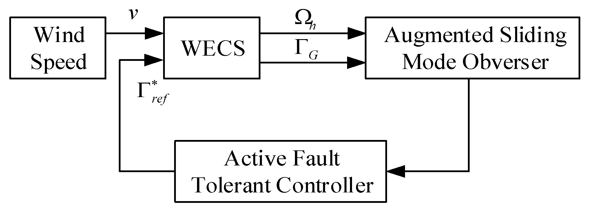
The overall block diagram of active fault-tolerant control for the WECS is shown in Figure 2.

The low power and high speed wind energy conversion system based on DFIG is adopted [26].

The simulation parameters are shown in

Table 1. Simulation Parameters.

Parameter Names	Parameter Values
Rated voltage VS	220 V
Rated speed wS	100 πrad/s
Rated electromagnetic torque ΓGmax	40 N·m
Electromagnetic time constant TG	0.02
Air density ρ	1.25 kg/m3
Transmission efficiency η	95%
Transmission speed ratio i0	6.25
Blade length R	2.5 m
Moment of interia of high speed axis Jt	0.0092 kg·m2
Moment of interia of low speed axis Jwt	3.6 kg·m2

:

At rated wind speed, fixed pitch control is adopted, that is β = 0°, the wind energy conversion coefficient C_p is determined by the following Equation (29):

$$\begin{array}{l}{C}_p(\lambda )=-4.54\times {10}^{-7}{\lambda }^7+1.3027\times {10}^{-5}{\lambda }^6-6.5416\times {10}^{-5}{\lambda }^5\\ -9.7477\times {10}^{-4}{\lambda }^4+8.1\times {10}^{-3}{\lambda }^3-1.3\times {10}^{-3}{\lambda }^2+6.1\times {10}^{-3}\lambda \end{array}$$

(29)

When the tip speed ratio is λ = 7, the maximum value is 0.476, which is the best tip speed ratio, where $d\left(x,u,t\right)={\left[\frac{8.5C_p\left(\lambda \right){\mathsf{\Omega }}_h^2}{{\lambda }^3} 0\right]}^T$.

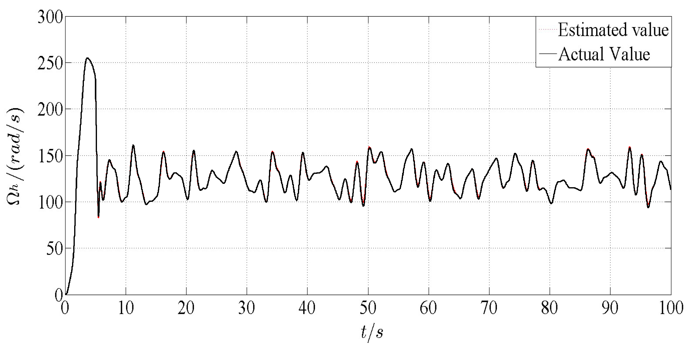
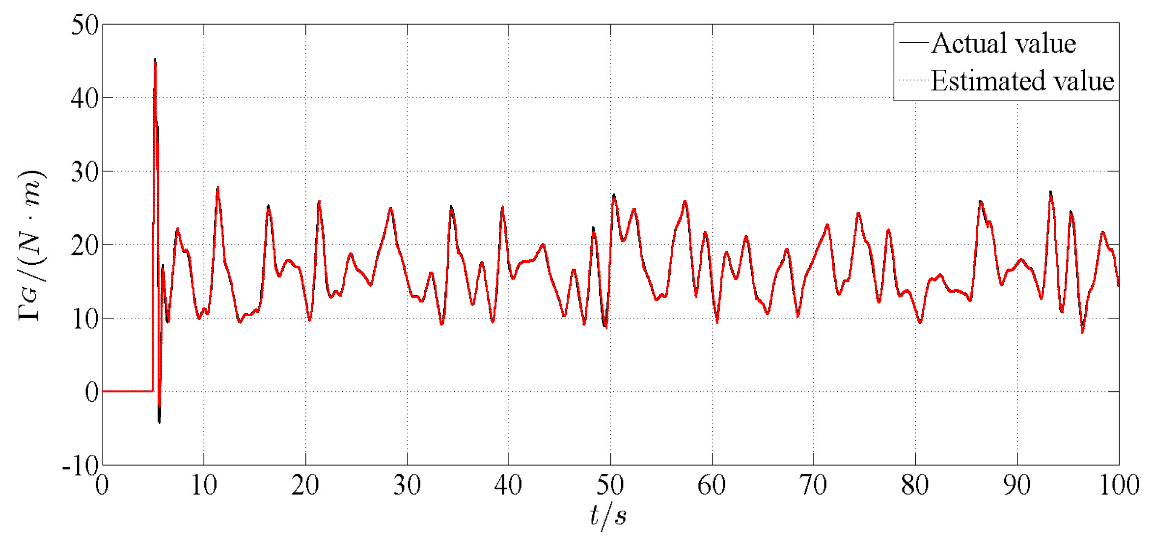
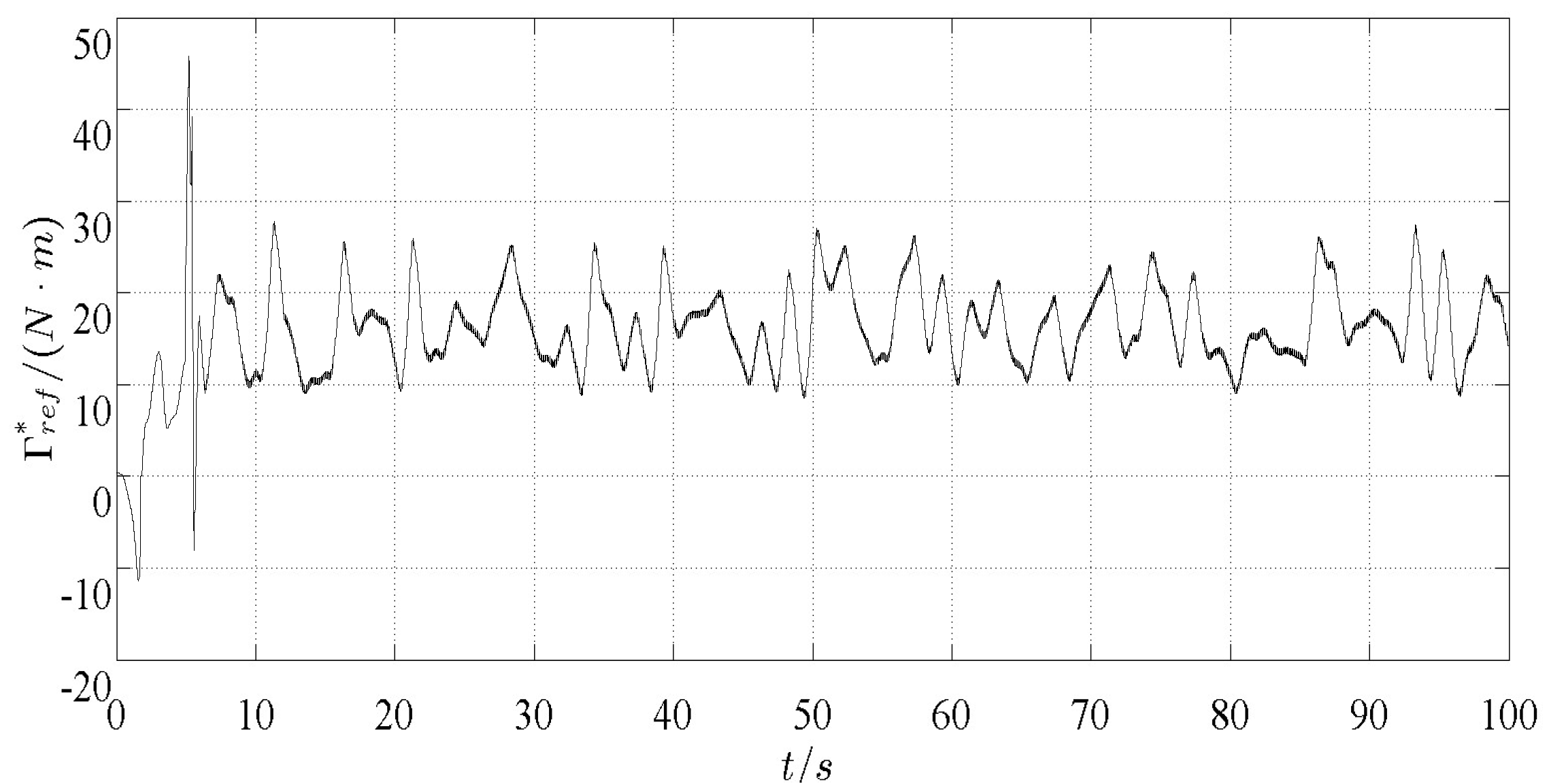
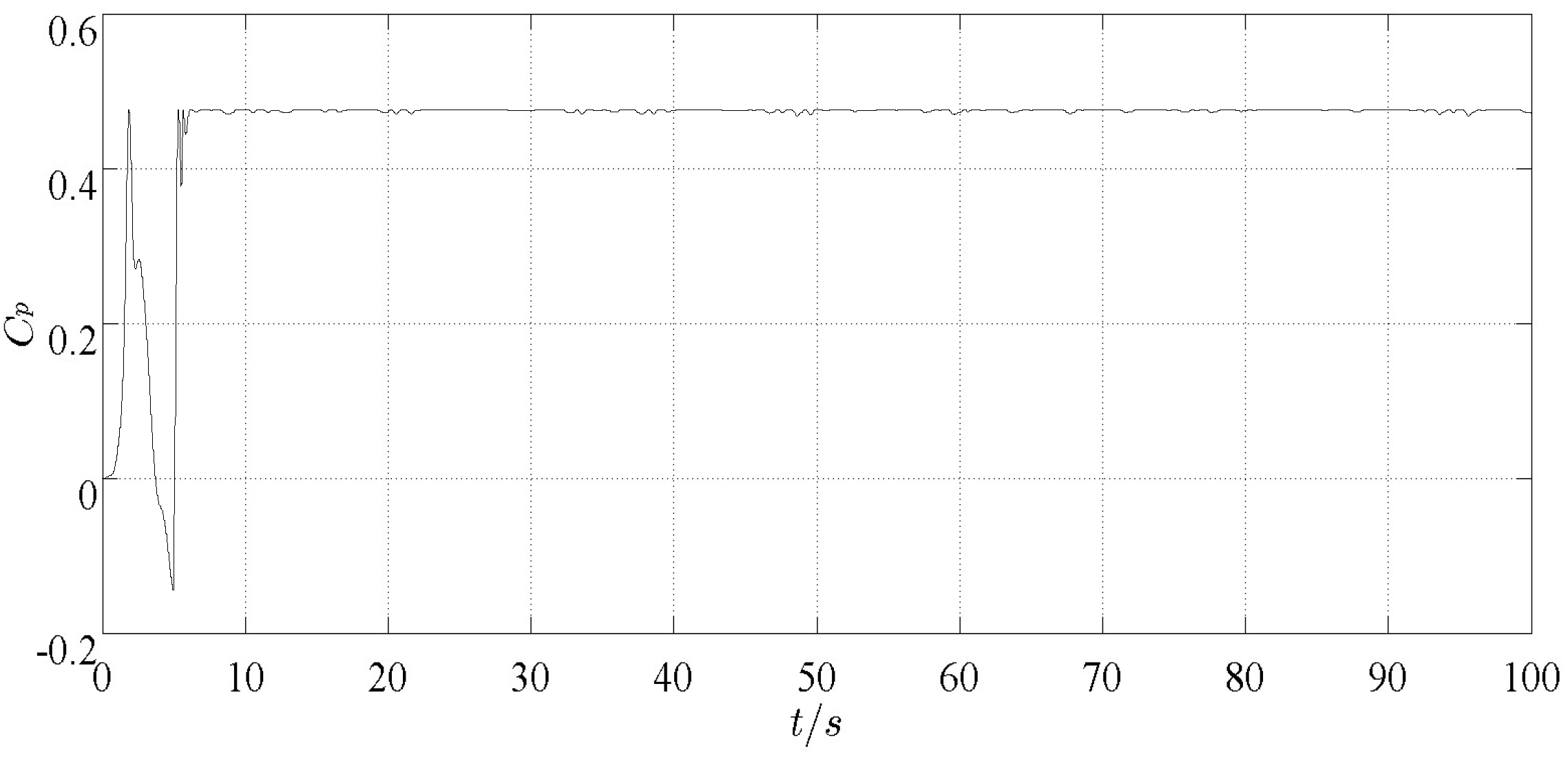
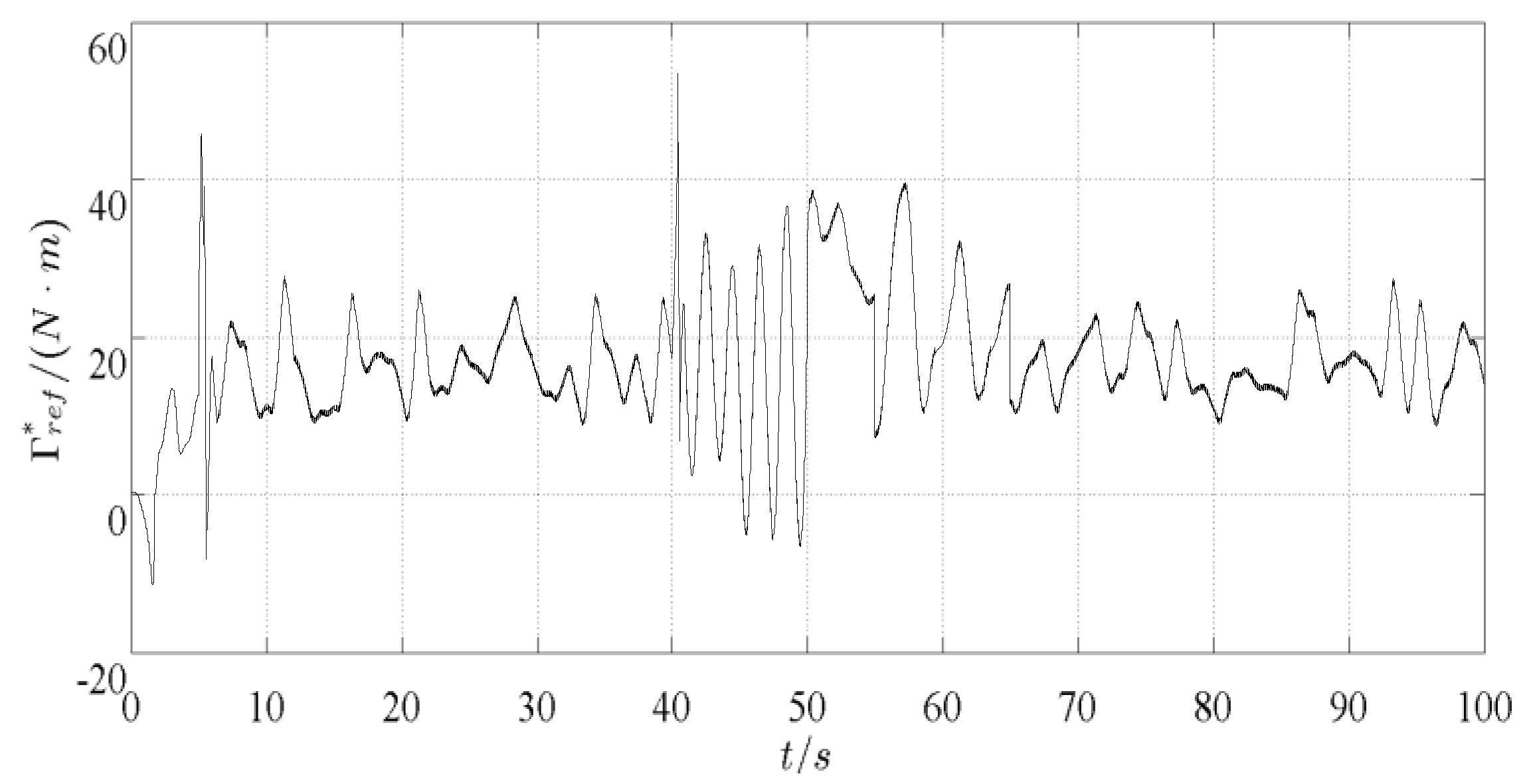
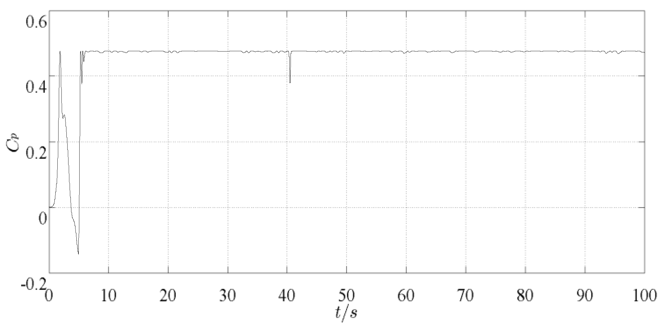
It can be seen that Figure 3 is a comparison of the estimated and actual values of the speed of the high-speed shaft speed when the system is fault-free. Figure 4 is a comparison of the estimated and actual values of the electromagnetic torque. As shown in Figure 3 and Figure 4, the sliding mode observer designed in this paper can quickly follow the original state of the system, and the effect of state estimation is satisfactory. The reference value of electromagnetic torque ${\mathsf{\Gamma }}_{ref}^{\ast }$ is shown in Figure 5, and the wind energy conversion coefficient C_p can reach the ideal maximum, which can be kept at about 0.476 in 5~100 s, as shown in Figure 6.

The common actuator faults of the WECS include deviation, drift and so on. Therefore, the simulation design considers the drift fault, deviation fault and the mixed fault function of the actuator, as follows:

$$f_a(t)=\{\begin{array}{l}15\sin \pi t 40\mathrm{s}\le t<50\mathrm{s}\\ 12 50\mathrm{s}\le t<55\mathrm{s}\\ 4.5+10\sin (0.8\pi t) 55\mathrm{s}\le t<65\mathrm{s}\end{array}$$

(30)

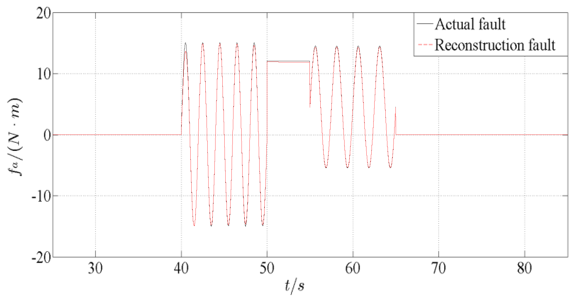
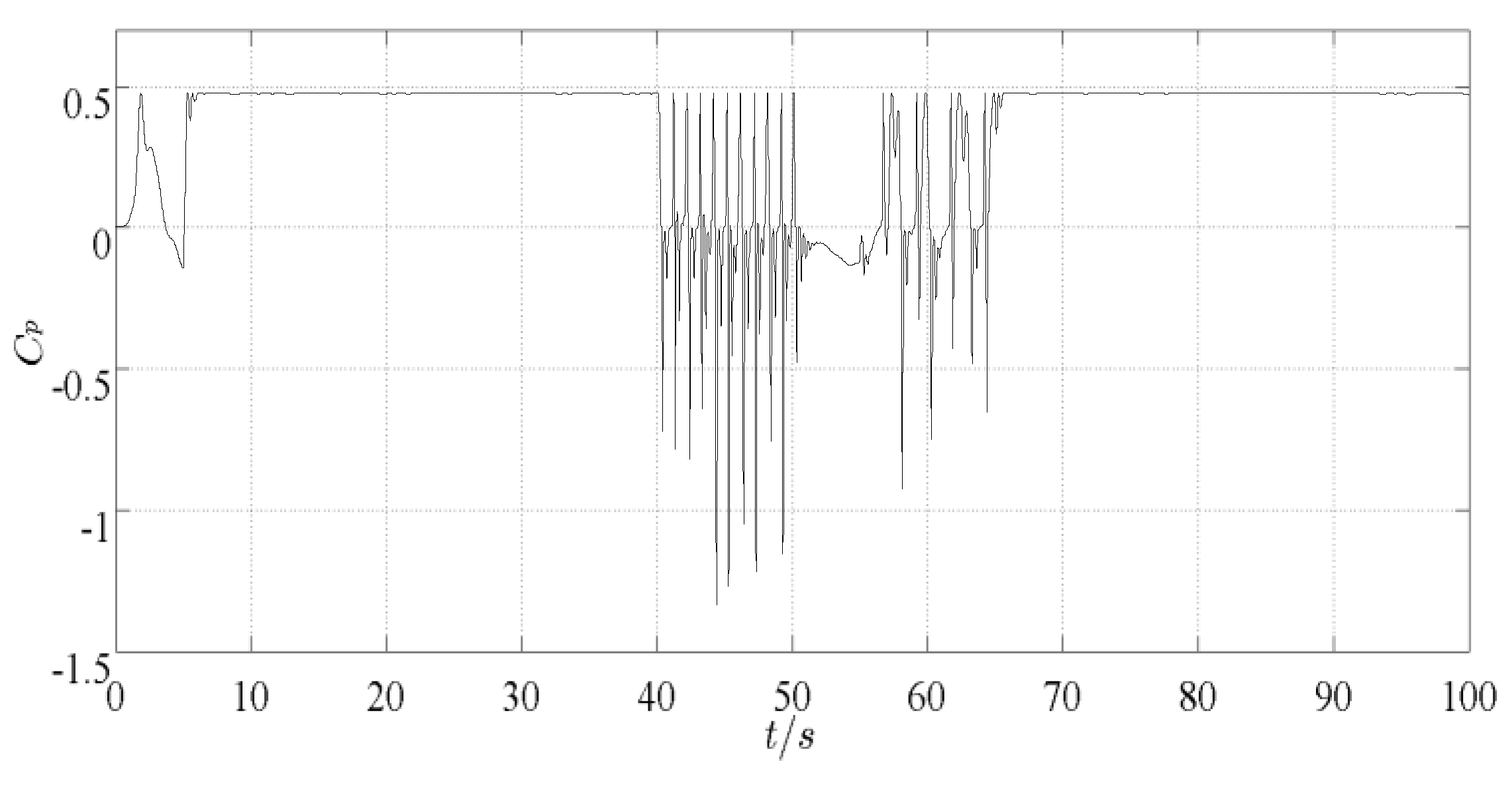
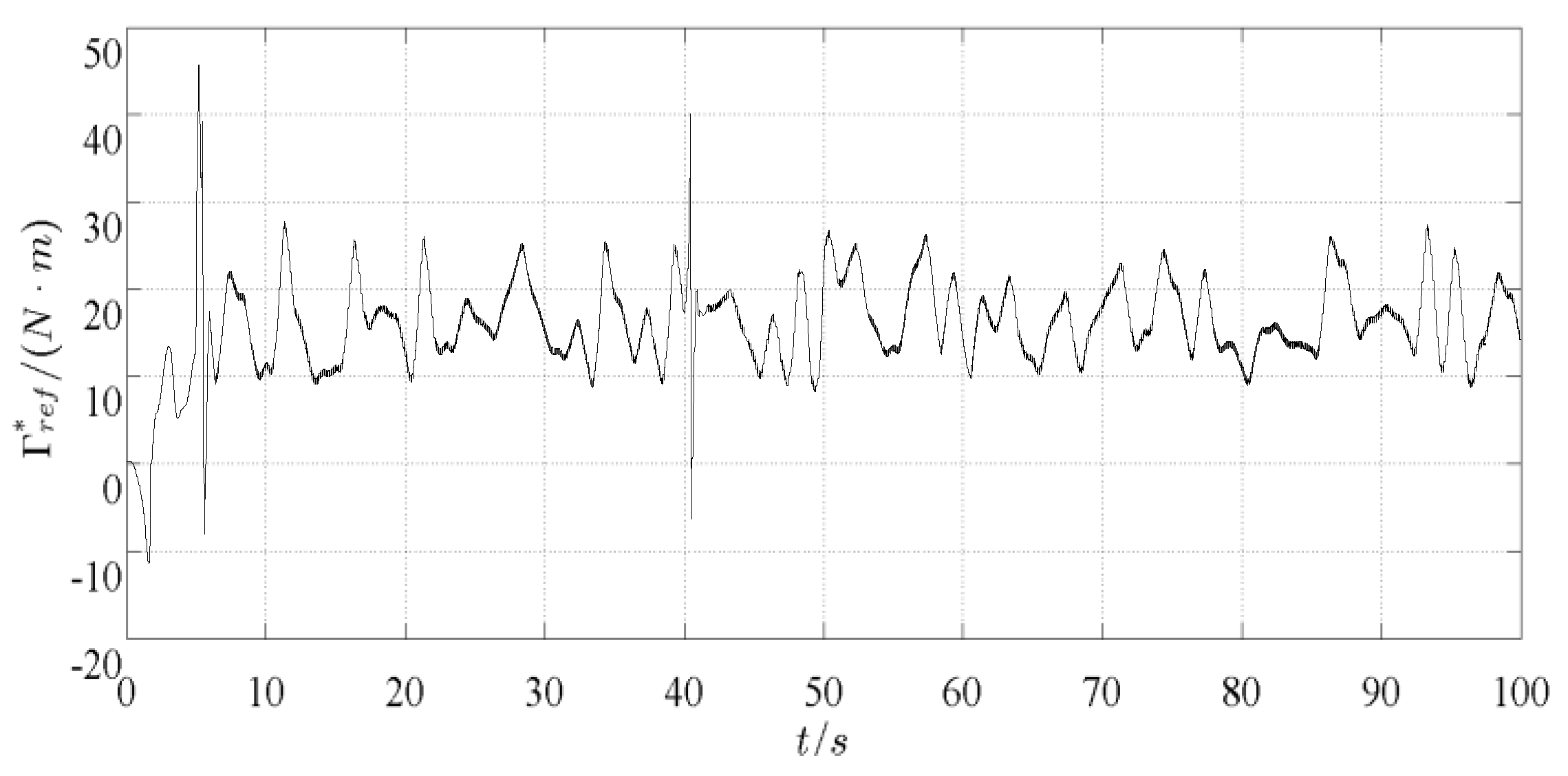
Figure 7 is a simulation comparison of actuator faults and their reconstructed values. From Figure 7, it can be seen that the augmented observer can accurately reconstruct the actuator fault of the WECS, and directly obtain the fault waveform, magnitude and other information. When the actuator fault occurs, the reference value of electromagnetic torque ${\mathsf{\Gamma }}_{ref}^{\ast }$ changes greatly, as shown in Figure 8. During the period of 40 s~65 s, the wind energy conversion coefficient has seriously deviated from the optimal value and has a large fluctuation range, which cannot be maintained in the optimal position, as shown in Figure 9. By comparing the fault value of performance parameters with that of intact fault-free values, it can be seen that when the actuator fault occurs, the performance of the WECS is affected to a certain extent, resulting in poor efficiency of wind energy conversion. Active fault-tolerant control can compensate the actuator fault better. The reference value of electromagnetic torque ${\mathsf{\Gamma }}_{ref}^{\ast }$ after fault-tolerant control can approximately follow the actual fault-free state, as shown in Figure 10. When the actuator fault occurs, the WECS can still achieve maximum capture. The tip speed ratio of the system fluctuates near 7 m/s. The fault-tolerant wind energy conversion coefficient is shown in Figure 11.

7. Conclusions

In this paper, the problem of state estimation and fault reconstruction for uncertain WECS are discussed when the actuator fault occurs. An augmented sliding mode observer is constructed by splitting the non-linear term of the state equation of the WECS into uncertain parts of the system and augmenting the state. Then the robust fault reconfiguration observer is designed, and the equivalent output method is used to reconstruct the actuator fault, which has strong robustness. The active fault-tolerant controller designed ensures the stable input of the system and captures the maximum wind energy.

References

- Attya, A.B.; Dominguez-Garcia, J.L.; Anaya-Lara, O. A review on frequency support provision by wind power plants: Current and future challenges. Renew. Sustain. Energy Rev. 2018, 34, 483–490. [Google Scholar] [CrossRef]
- Yang, Z.; Chai, Y. A survey of fault diagnosis for onshore grid-connected converter in wind energy conversion systems. Renew. Sustain. Energy Rev. 2016, 66, 345–359. [Google Scholar] [CrossRef]
- Hang, J. An Overview of Condition Monitoring and Fault Diagnostic for Wind Energy Conversion System. Trans. China Electrotech. Soc. 2013, 28, 261–271. [Google Scholar]
- Kamal, E.; Aitouche, A. Robust fault tolerant control of DFIG wind energy systems with unknown inputs. Renew. Energy 2013, 56, 2–15. [Google Scholar] [CrossRef]
- Vidal, Y.; Christian, T.; José, R.; Acho, L. Fault Diagnosis and Fault-Tolerant Control of Wind Turbines via a Discrete Time Controller with a Disturbance Compensator. Energies 2015, 8, 4300–4316. [Google Scholar] [CrossRef] [Green Version]
- Kamal, E.; Aitouche, A.; Ghorbani, R.; Bayart, M. Robust fuzzy fault-tolerant control of wind energy conversion systems subject to sensor faults. IEEE Trans. Sustain. Energy 2012, 3, 231–241. [Google Scholar] [CrossRef]
- Badihi, H.; Zhang, Y.; Hong, H. Wind Turbine Fault Diagnosis and Fault-Tolerant Torque Load Control Against Actuator Faults. IEEE Trans. Control Syst. Technol. 2015, 23, 1351–1372. [Google Scholar] [CrossRef]
- Wu, D.; Jin, S.; Shen, Y.; Ji, Z. Active fault-tolerant linear parameter varying control for the pitch actuator of wind turbines. Nonlinear Dyn. 2017, 87, 475–487. [Google Scholar] [CrossRef]
- Wu, Z.Q.; Yang, Y.; Xu, C.H. Adaptive fault diagnosis and active tolerant control for wind energy conversion system. Int. J. Control Autom. Syst. 2015, 13, 120–125. [Google Scholar] [CrossRef]
- Benbouzid, M.E.H.; Beltran, B.; Amirat, Y.; Yao, G.; Han, J.; Mangel, H. Second-order sliding mode control for DFIG-based wind turbines fault ride-through capability enhancement. ISA Trans. 2014, 53, 827–833. [Google Scholar] [CrossRef] [Green Version]
- Mekri, F.; Elghali, S.B.; Benbouzid, M.E.H. Fault-Tolerant Control Performance Comparison of Three- and Five-Phase PMSG for Marine Current Turbine Applications. IEEE Trans. Sustain. Energy 2013, 4, 425–433. [Google Scholar] [CrossRef] [Green Version]
- Beltran, B.; Benbouzid, M.E.H.; Ahmed-Ali, T. Second-order sliding mode control of a doubly fed induction generator driven wind turbine. IEEE Trans. Energy Convers. 2012, 27, 261–269. [Google Scholar] [CrossRef]
- Benelghali, S.; Benbouzid, M.; Charpentier, J.F.; Ahed-Ali, T.; Munteanu, I. Experimental Validation of a Marine Current Turbine Simulator: Application to a Permanent Magnet Synchronous Generator-Based System Second-Order Sliding Mode Control. IEEE Trans. Ind. Electron. 2011, 58, 118–126. [Google Scholar] [CrossRef] [Green Version]
- Ha, Q.P.; Trinh, H. State and input simultaneous estimation for a class of nonlinear systems. Automatica 2004, 83, 1779–1785. [Google Scholar] [CrossRef]
- Lee, D.J.; Park, Y.J.; Youn, S. Robust H∞ sliding mode descriptor observer for fault and output disturbance estimation of uncertain systems. IEEE Trans. Autom. Control 2012, 57, 2928–2934. [Google Scholar] [CrossRef]
- Zhang, J.; Shi, P.; Lin, W. Extended sliding mode observer based control for Markovian jump linear systems with disturbances. Automatica 2016, 70, 140–147. [Google Scholar] [CrossRef]
- Gao, Z.; Liu, X.; Chen, M.Z.Q. Unknown Input Observer-Based Robust Fault Estimation for Systems Corrupted by Partially Decoupled Disturbances. IEEE Trans. Ind. Electron. 2016, 63, 2537–2547. [Google Scholar] [CrossRef]
- Alipouri, Y.; Poshtan, J.; Zarch, M.G. Generalized Sliding Mode with Integrator Controller Design Using a Discrete Linear Model. Proc. Inst. Mech. Eng. Part I J. Syst. Control Eng. 2014, 228, 677–689. [Google Scholar] [CrossRef]
- Zhang, K.; Jiang, B. Fault Diagnosis Observer-based Output Feedback Fault Tolerant Control Design. Acta Autom. Sin. 2010, 36, 274–281. [Google Scholar] [CrossRef]
- Liu, X.; Gao, Z.; Chen, M. Takagi-Sugeno Fuzzy Model Based Fault Estimation and Signal Compensation with Application to Wind Turbines. IEEE Trans. Ind. Electron. 2017. [Google Scholar] [CrossRef]
- Carroll, J.; Mcdonald, A.; Mcmillan, D. Reliability Comparison of Wind Turbines with DFIG and PMG Drive Trains. IEEE Trans. Energy Convers. 2015, 30, 663–670. [Google Scholar] [CrossRef]
- Qu, Y.B.; Song, H.H. Energy-based coordinated control of wind energy conversion system with DFIG. Int. J. Control 2011, 84, 2035–2045. [Google Scholar] [CrossRef]
- Kenyon, M. Energy-Reliability Optimization of Wind Energy Conversion Systems by Sliding Mode Control. IEEE Trans. Energy Convers. 2008, 23, 975–985. [Google Scholar]
- Zhang, Z.; Verma, A.; Kusiak, A. Fault Analysis and Condition Monitoring of the Wind Turbine Gearbox. IEEE Trans. Energy Convers. 2012, 27, 526–535. [Google Scholar] [CrossRef] [Green Version]
- Shen, Q.; Jiang, B.; Cocquempot, V. Adaptive Fuzzy Observer-Based Active Fault-Tolerant Dynamic Surface Control for a Class of Nonlinear Systems with Actuator Faults. IEEE Trans. Fuzzy Syst. 2014, 22, 338–349. [Google Scholar] [CrossRef]
- Munteanu, I.; Bratcu, A.I.; Cutululis, N.-A.; Ceanga, E. Optimal Control of Wind Energy Systems; Springer: London, UK, 2008. [Google Scholar]
Figure 1.
Wind energy conversion system (WECS) based on Doubly fed induction generator (DFIG).
Figure 2.
Overall block diagram of fault-tolerant control for the WECS.
Figure 3.
Actual and estimated values of speed Ωh of high speed shaft.
Figure 4.
The actual and estimated values of electromagnetic torque ΓG.
Figure 5.
Reference value of electromagnetic torque without fault.
Figure 6.
Wind energy conversion coefficient value Cp without fault.
Figure 7.
Actual and reconstructed values of actuator fault fa.
Figure 8.
Reference value of electromagnetic torque when actuator fails.
Figure 9.
Wind energy conversion coefficient value Cp when actuator fails.
Figure 10.
Reference value of electromagnetic torque after fault-tolerant control.
Figure 11.
Wind Energy Conversion Coefficient Value Cp without Fault after Fault Tolerant Control.