A Remotely Controlled Sea Level Compensation System for Wave Energy Converters

1
Swedish Centre for Renewable Electric Energy Conversion, Division of Electricity, Department of Engineering Sciences, The Angstrom Laboratory, P.O Box 534, SE-75121 Uppsala, Sweden
2
School of Mechatronic Engineering, Universiti Malaysia Perlis, Arau 02600, Perlis, Malaysia
*
Author to whom correspondence should be addressed.
Energies 2019, 12(10), 1946; https://doi.org/10.3390/en12101946
Submission received: 10 April 2019
/
Revised: 14 May 2019
/
Accepted: 15 May 2019
/
Published: 21 May 2019
(This article belongs to the Special Issue Marine Tidal and Wave Energy Converters: Technologies, Conversions, Grid Interface, Fault Detection, and Fault-Tolerant Control)
Abstract
:The working principle of the wave energy converter (WEC) developed at Uppsala University (UU) is based on a heaving point absorber with a linear generator. The generator is placed on the seafloor and is connected via a steel wire to a buoy floating on the surface of the sea. The generator produces optimal power when the translator’s oscillations are centered with respect to the stator. However, due to the tides or other changes in sea level, the translator’s oscillations may shift towards the upper or lower limit of the generator’s stroke length, resulting in a limited stroke and a consequent reduction in power production. A compensator has been designed and developed in order to keep the generator’s translator centered, thus compensating for sea level variations. This paper presents experimental tests of the compensator in a lab environment. The wire adjustments are based on online sea level data obtained from the Swedish Meteorological and Hydrological Institute (SMHI). The objective of the study was to evaluate and optimize the control and communication system of the device. As the device will be self-powered with solar and wave energy, the paper also includes estimations of the power consumption and a control strategy to minimize the energy requirements of the whole system. The application of the device in a location with high tides, such as Wave Hub, was analyzed based on offline tidal data. The results show that the compensator can minimize the negative effects of sea level variations on the power production at the WEC. Although the wave energy concept of UU is used in this study, the developed system is also applicable to other WECs for which the line length between seabed and surface needs to be adjusted.
1. Introduction
Research on the production of electrical energy from ocean waves has evolved significantly over the years, with the development and testing of various types of wave energy converters (WECs). Different techniques and strategies have been implemented in order to improve the performance of WECs both at the simulation and theoretical level [1,2,3,4] and at the sea testing level [5,6,7]. The analysis and the evaluation of the performance of WEC technologies have also been studied and can be referred to previously-published works; see [8,9,10]. At Uppsala University, the studied and developed WEC is a heaving-point-absorbing-type converter.
The first version of the sea level compensator from Uppsala University, which was dimensioned for the climate of the Swedish west coast, has been tested [11]. A study by Castellucci [12] analyzed the effect of sea level changes on the absorption of wave energy. The result from the study showed that the implementation of the compensator significantly improved energy production.
This paper focuses on the next-generation tidal compensator for Uppsala University WECs. The tidal compensator is dimensioned to work in the Welsh Sea, which is characterized by a semi-diurnal tidal range of up to 6.6 m [13]. Because of the high tidal range, a higher range tidal compensator for the Uppsala University WEC is needed. In optimal operating conditions, the translator oscillates centered to the mean position of the generator, with the changes in water level (tides) causing the translator to shift towards the top or the bottom of the generator, thereby reducing the efficiency of the WEC.
The compensator consists of a pocket wheel hosting a steel chain and a gearbox. The system is driven by a DC motor rated at 1500 W. A steel chain of 9 m connects the compensator to the buoy line. This chain rolls over the pocket wheel to adjust the length of the buoy line. The gearbox is located between the pocket wheel and a DC motor via a steel shaft. Because of a total load (translator and buoy line) of 10 tonnes, a gearbox with a reduction ratio of 4758 has been used [14]. This can increase the lifting torque (or force) significantly without compromising the ability of the system to adjust the buoy line according to the tidal level.
In order to protect the sensitive parts from corrosion, only the chain and the pocket wheel are allowed to be exposed to the sea water. All three parts (pocket wheel, chain, and shaft) are made of non-corrosive material. The rest of the system is covered by a protective casing. To prevent the sea water from entering the casing, two pairs of U-shaped sealings have been installed.
The real-time experimental test in the lab environment was carried out on the basis of the sea level data at Brofjorden [15]. The sea level at Brofjorden has been chosen as it is the closest measurement station to the Lysekil wave energy research site, located around 12 km to the south. For the adaptation of the system to higher ranges of sea level variation, offline information on tidal levels from a station close to Wave Hub has been analyzed. Offline sea level data from the Newlyn Tidal Observatory obtained from the British Oceanographic Data Centre (BODC) [13] have been used to simulate the compensator’s operation at Wave Hub. The Newlyn station is located 22 km south of Wave Hub. The time series analyzed was one year long (from May 2017 until April 2018) with a 15-minute temporal resolution.
This paper presents the simulations and lab experiments on the compensator system based on the sea level information published by the Swedish Meteorological and Hydrological Institute (SMHI) and the BODC. The Methods Section explains the experimental setup of the compensator in the lab environment, followed by the operational test of the compensator. The accuracy of the chain position and the analysis of the power consumption are presented in the Results Section.
2. Methods
This section is divided into three subsections. Section 2.1 describes the communication and control strategy. Section 2.2 provides the experimental setup, describing the sensors and the testing for static and dynamic operation. Section 2.3 models the behavior of the motor to estimate the power consumption.
2.1. Communication and Control Strategy
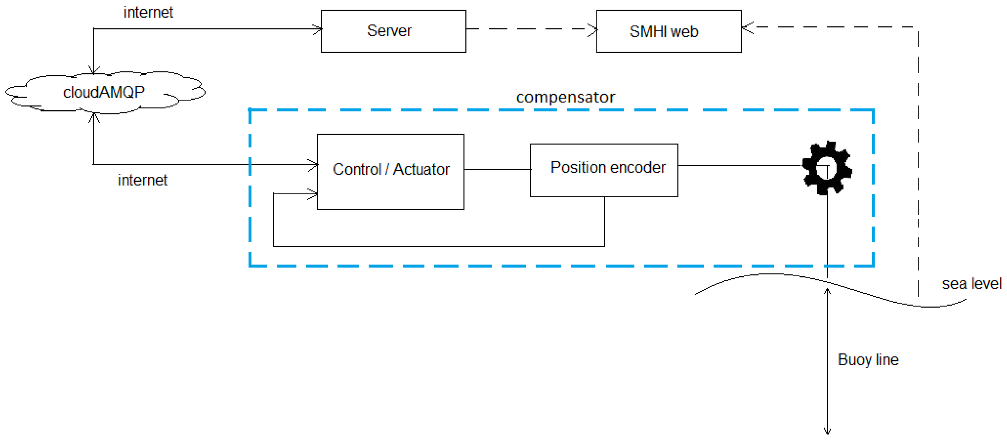
A server for the compensator system was set up to log the data and to handle the control strategy for the compensator. A simplified block diagram of the communication and control flows is shown in Figure 1.
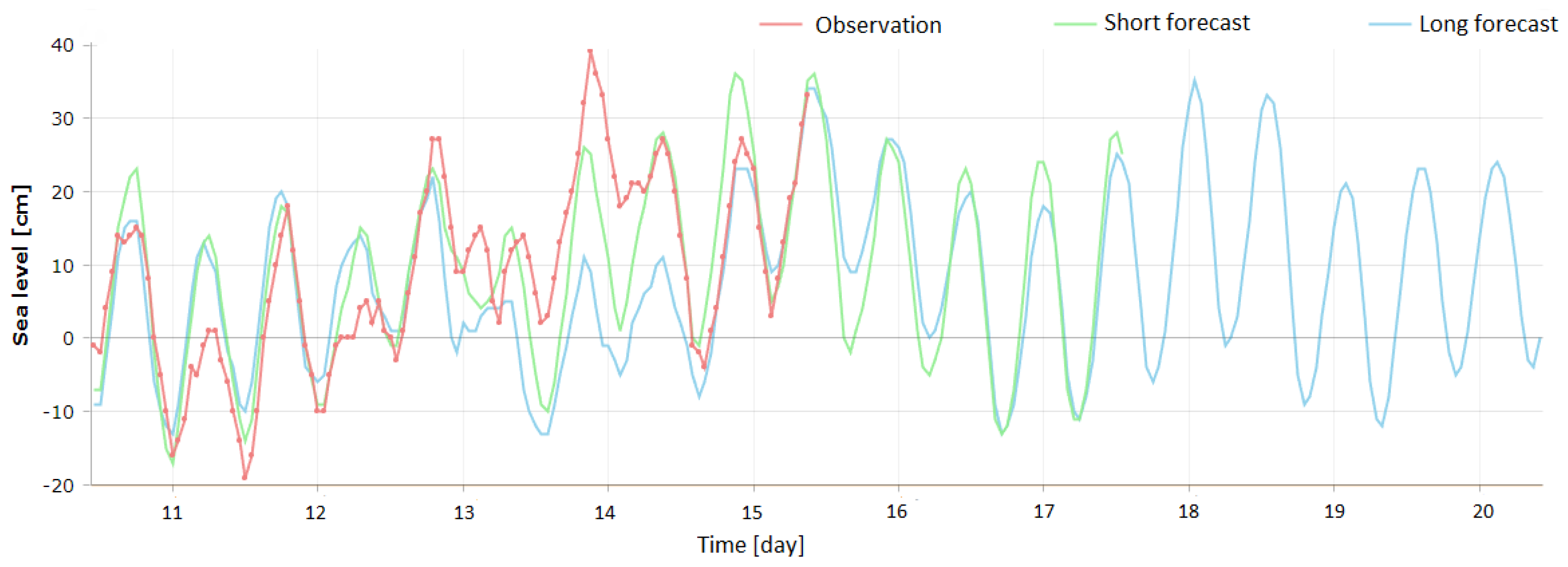
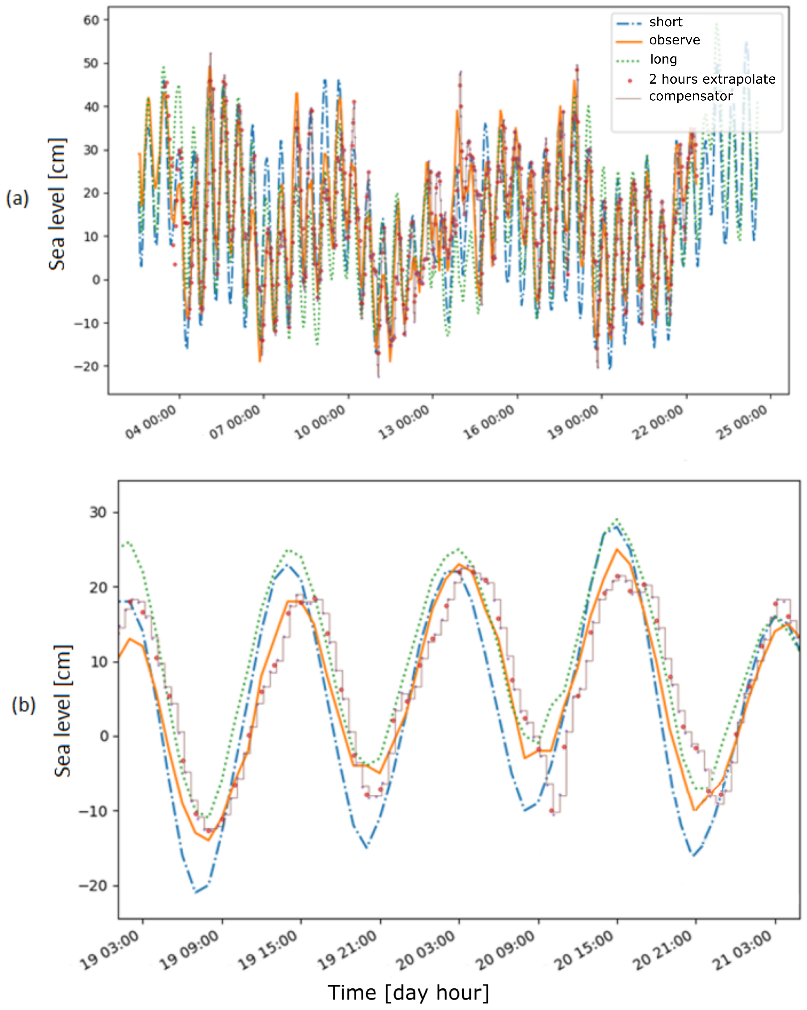
The input parameter of the system is the sea level, collected online from the SMHI website [15] (see Figure 3). The observed sea level data published on the website lag between 1 and 2 h. In addition to the observed data, two other types of data series are made available by the SMHI, namely short-forecast data and long-forecast data. The easiest way to control the compensator would be to follow the short-forecast data as the observed data are not published in real time, whereas the forecast data are available ahead of the current time. However, it can be seen from Figure 3 that there is a noticeable variation between the sea level that is observed at the station and the sea level that is forecasted. To minimize this variation, a prediction model using least-squares minimization was employed to predict the current sea level up to 2 h in advance based on the observed sea level data series.
The prediction of the current sea level data was based on the observational data from the SMHI. Because sea level variations can, in general, be considered to be periodic, a moving frame with a sinusoidal shape for the sea level was used to obtain the data for the next two hours (sea level at the present time). The illustration of this procedure is shown in Figure 4.
The rectangular frame shows how 10 observations were used to extrapolate the subsequent data point. The least-squares minimization method [17] was used to fit these 10 observations to get the best fit of a sine function. The acquired sine function was then used to extrapolate the next 2 h of data points every hour (up to the present time) (see Figure 4). The frame was shifted one hour when new observational data were obtained from the SMHI. This process was repeated to predict the sea level data points of the next hour continuously. A simulation to analyze the difference between the extrapolated data and the observed and forecasted data was performed for a period of 19 days.
2.1.1. Server
The system server was placed on land. This was the main component of the communication and control system. The server reads the sea level information from the SMHI website, does the analysis, and makes a prediction of the seal level for up to 2 h in advance based on the SMHI observations. The SMHI updates the observational data on an hourly basis, so the server accesses the website once every hour. The communication between the server and the compensator is done via the cloud service cloudAMQP [18] based on RabbitMQ.
2.1.2. CloudAMQP
CloudAMQP is a cloud server developed by a Swedish tech company. CloudAMQP handles message queues based on the RabbitMQ protocol (open source multi-protocol messaging broker). A basic account from this cloud service with limited connection and queue data is enough to handle the small-sized data exchange between the server and the compensator. For our application, the compensator kept sending the status of the sensor readings (and position information) to the cloudAMQP. These data were then forwarded to the server at Uppsala University. The same protocol was used to send commands regarding the chain’s current and future positions from the server to the compensator. The advantage of using this cloud messaging service is its simplicity. The communication between the server and the compensator is asynchronous.
2.2. Experimental Setup
Figure 2 shows the schematic of the components installed in the compensator device. Every component has been explained in detail in [16]. In general, the heart of the control is the Arduino Mega2560 [19], which is linked together with other components to a single-board computer (Raspberry Pi) used for communication via a 3G dongle. The compensator sends the status to the server (via cloudAMQP) at a frequency of 1 Hz. Raspberry-pi can also be accessed manually by VPN using the RealVNC application. However, normally, the automated operation of the compensator cloudAMQP was chosen.
The Arduino Mega2560 was chosen as the main controller due to its low cost and the fact that it is open source and easy to integrate with other systems. As the control system for the compensator does not need high processing power and several input/output ports, the Arduino seems suitable. Raspberry Pi was used as the onboard computer with the purpose of performing data logging and Internet communication. Because of its low power consumption and its potential to control and operate remotely, Arduino has been used for the Internet of Things (IoT) application in real-time data monitoring and management, e.g., the photovoltaic (PV) systems monitoring, as described in [20,21].
2.2.1. Encoder as a Position Sensor
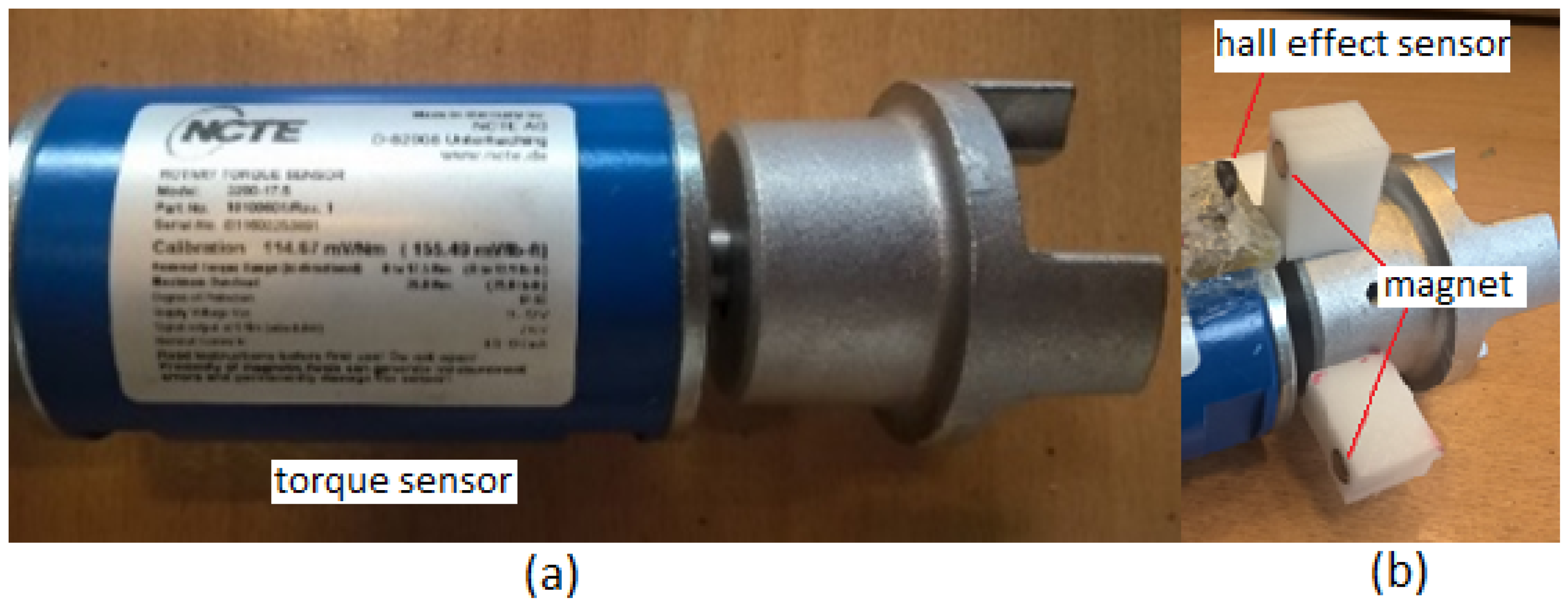
A rotary encoder was used to calculate the rotation of the motor shaft and, subsequently, to calculate the motor rpm and position of the chain. A Hall effect sensor was mounted to face a rotating axis of two permanent magnets with the poles facing opposite directions. Figure 5 shows the setup for the encoder.
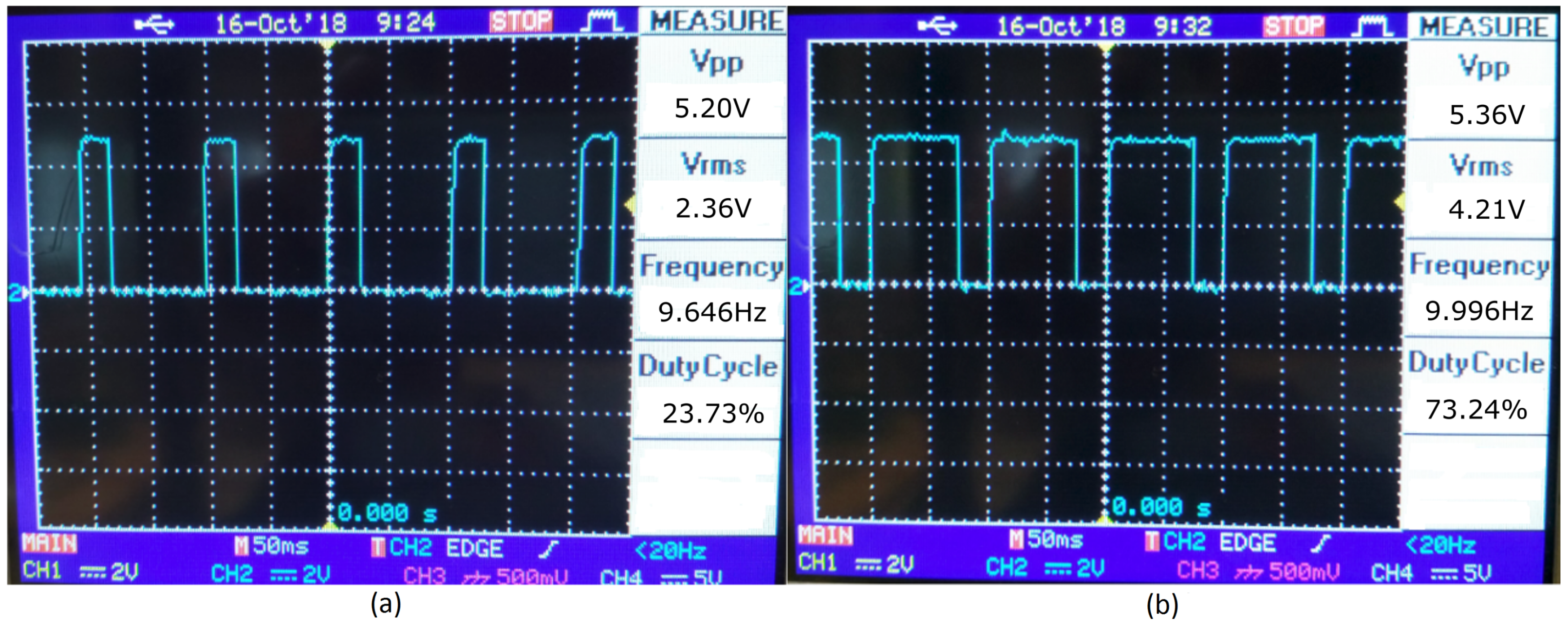
The two permanent magnets were installed apart from the rotating coupler in order to obtain a fixed duty cycle of the output signal regardless of the speed of the motor shaft. From this output, the direction and the speed of rotation could be calculated. The sensitivity of the encoder was one pulse per revolution. This was translated to a 0.2-mm resolution of the buoy line position. Figure 6 shows 2 waveform samples from the encoder signal. The output from the encoder was fed to the Arduino for a feedback measurement. Table 1 shows the information obtained from the encoder measurement.
The position of the magnet was placed so that when the motor turns clockwise (CW), the encoder will always generate approximately a 25% duty cycle. Conversely, when the motor turns counter-clockwise (CCW), the encoder generates signals of a 75% duty cycle. The information of the duty cycle and frequency from the encoder was used to determine the direction, the speed, and the position of the motor when lifting and releasing the load. The position of the chain was saved every time the Raspberry Pi received inputs from Arduino in order to protect the system from data loss, in case it was reset. A secondary position measurement system was also installed: a draw-wire sensor (DWS) was mounted on the low-speed side of the gearbox (12 cm-diameter shaft). The wire was wound over the shaft and was able to give the absolute position value when needed. However, the draw wire sensor was not as accurate as the encoder and can be used as a backup if the encoder system fails.
2.2.2. Force Measurement
The compensator was designed to be able to bear the weight of the translator and the connection line, which resulted in a total of 10 tonnes. A torque sensor (Figure 5) [22] was installed to measure the torque and estimate the force exerted on the chain. The nominal range for this torque sensor was 17 Nm, which translates to about 83 kNm at the output of the gearbox. The torque sensor was installed at the coupling between the DC motor’s shaft and the gearbox.
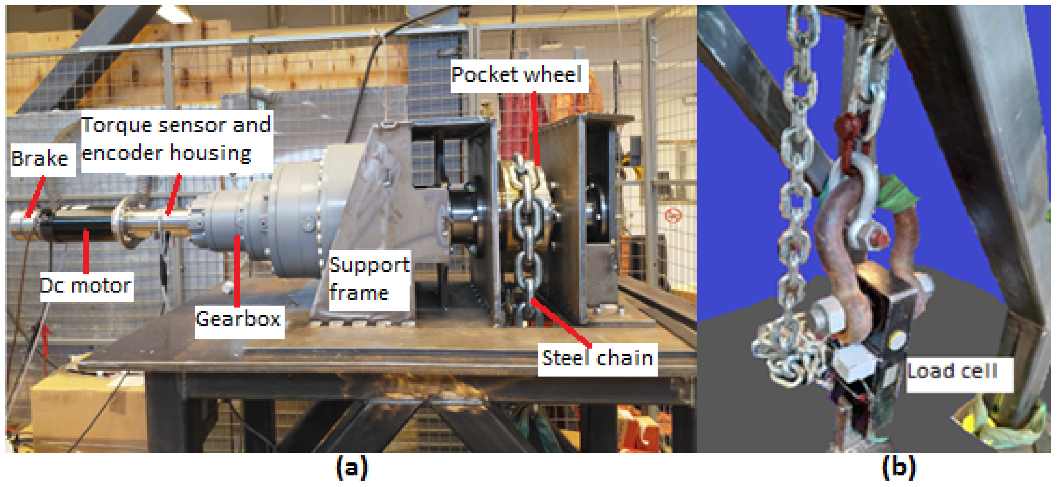
In order to test the torque sensor, experiments were carried out. The lab environment with the setup is shown in Figure 7. Doing dynamic tests on the compensator using the real load conditions is complicated and poses safety risks; hence, static tests were performed using a load cell mounted on the floor. The load cell shown in Figure 7 was rated at 25 tonnes.
For the static tests, one side of the load cell was connected to the chain and the other end to the floor, as shown in Figure 7. During the test, the load cell was pulled by the chain to measure the pulling force on the compensator. The result of this experiment, shown in Figure 8, was used to calibrate the torque sensor: the force measured by the load cell should be equal to the force calculated from the output of the torque sensor. Even though the gearbox turn ratio was high, the pull of the load on the torque sensor cannot be ignored. From the test, the instantaneous force applied by the chain was represented by the pull of the spring in the releasing-load direction (in the dynamic test) when the motor was stopped, and from the results, it was shown that the comparison of the forces measured at the spring and forces obtained from the torque sensor matched to an acceptable accuracy [16].
2.3. Power Consumption Estimation
The power consumption is one of the constraints for the system’s operation. The performance analysis of the system is focused on estimating the power consumption. To do so, the motor behavior was modeled in steady-state operation. Because the rate of sea level change is low, a fast response of the system is not necessary. The total power consumption was due to (a) the power consumption of the motor and the brake release when moving the chain and (b) the standby power necessary for monitoring and communication. The brake was powered only when the motor moved. At 24 V, the brake draws around 2 A current. Thus, the energy required for brake release is:
where t is the time it takes to complete the operation. The response of the motor was analyzed only in the steady-state condition. An experiment to characterize the system was performed by lifting a 35-kN load. The details of the test can be found in [16].
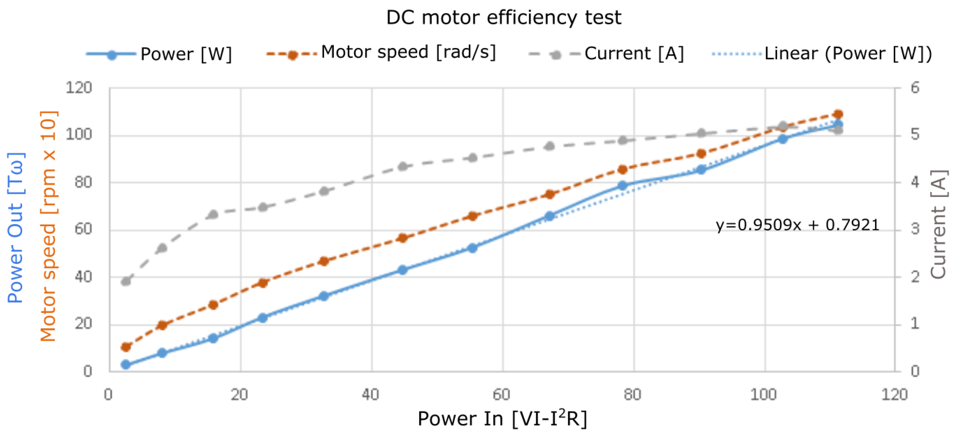
The relationship between the current, I, and the torque, T, can be obtained by measuring the torque when different currents are fed into the motor. This dynamic test to find the relation of I and T is plotted and shown in Figure 9. From the figure, it is noticeable that, in general, the torque was directly proportional to the current fed in. Ideally, the linear fit shown in Figure 9 should cross the origin, but in the experiment, a small current was required to overcome the internal friction of the motor before it started to turn. A static test was easier to determine the torque constant, but this dynamic test was more accurate to estimate the relation between I and T accounting for the effect of dynamic loses. The linear fit in Figure 9 shows the relation of I and T as:
With the same test, by considering the main loses of the DC motor to be the copper loses, where the resistance Ohm, the relationship between the input power to the motor and the output power calculated with the torque measurements can be obtained. The results are shown in Figure 10.
The significant losses of the system were considered to be copper losses, which were proportional to the square value of the current in the rotor windings. However, from the experiment, the efficiency of the motor, , after the copper losses had been accounted for, was found to be around 95 percent. The output power of the motor, , measured at the output motor shaft can be estimated as:
Expanding Equation (3) yields:
From Equation (4), can also be presented as the power exerted on the motor shaft from the perspective of the load. At steady state,
where is the power needed to operate the system without load. is the power needed to lift the translator, and is the dynamic efficiency of the compensator. The value of has been obtained from experimental (no load) tests. In order to estimate the power when the translator is lifted (or released) at a constant speed, , Equation (5) can be presented as:
where is the efficiency of the system, is the weight of the translator (100 kN), and v is the linear speed of the chain at . From Equation (6), the total power on the right-hand side can be estimated and is equal to . Because is known and the torque, , of the motor is proportional to the current I, the value of the required current can be obtained; the required voltage can subsequently be determined by equating to the left-hand side of Equation (6). Then, the power consumption to run the motor with load at speed can be estimated.
3. Results
Section 3.1 will present the simulation and experimental results of the compensator positioning for Brofjorden’s sea level. The effects on power consumption from different control strategies is presented in Section 3.2. Finally, the selected control strategy is adopted for Wave Hub and its effect on power consumption is analyzed in Section 3.3.
3.1. Compensator Positioning
Figure 11 shows the result from the simulation of the compensator position together with the sea level information from the SMHI for a duration of 19 days.
Table 2 shows the error analysis of long-forecast, short-forecast, and extrapolated sea levels compared to the observed data from the SMHI. The result of the root mean squared error (RMSE) analysis shows that the RMSE of the extrapolation from the observed data gave the smallest error, as compared with the error calculated for the short- and long-forecast data. Therefore, the first method was used to calculate the new position of the chain. Although the extrapolation left a margin of error, this will not significantly influence the power production, as discussed in a previous study on the impact of tidal levels on the WEC power production [12].
The user can set the parameters, as shown in Figure 12. By setting the interval time, the server will run fully automatically, reading SMHI information, continuously extrapolating the new position every hour, and sending commands to the compensator. There are several other parameters available on the GUI for manual positioning and safety.
Figure 13 shows the experimental results from a chain positioning test. The experiment was held in the lab environment without the translator load for a duration of two days. The purpose of the experiment was to evaluate the communication and the positioning control of the system. The result shows that the compensator could follow the sea level changes in real-time operation.
3.2. Power Consumption with Different Control Strategies
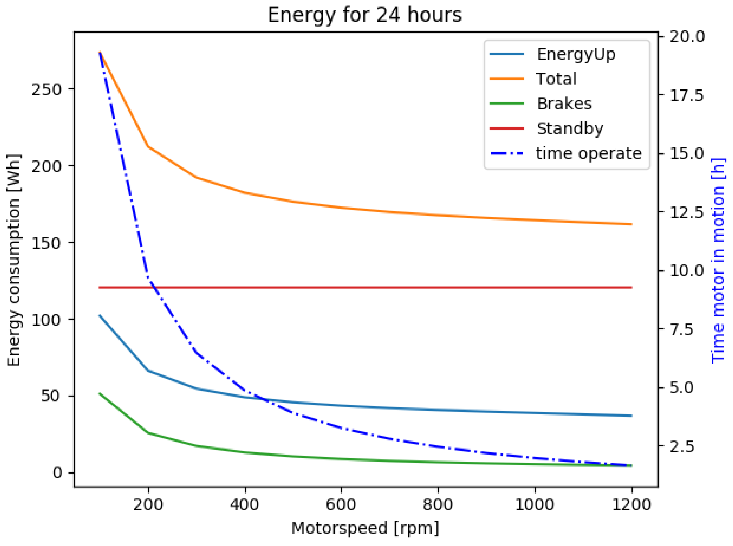
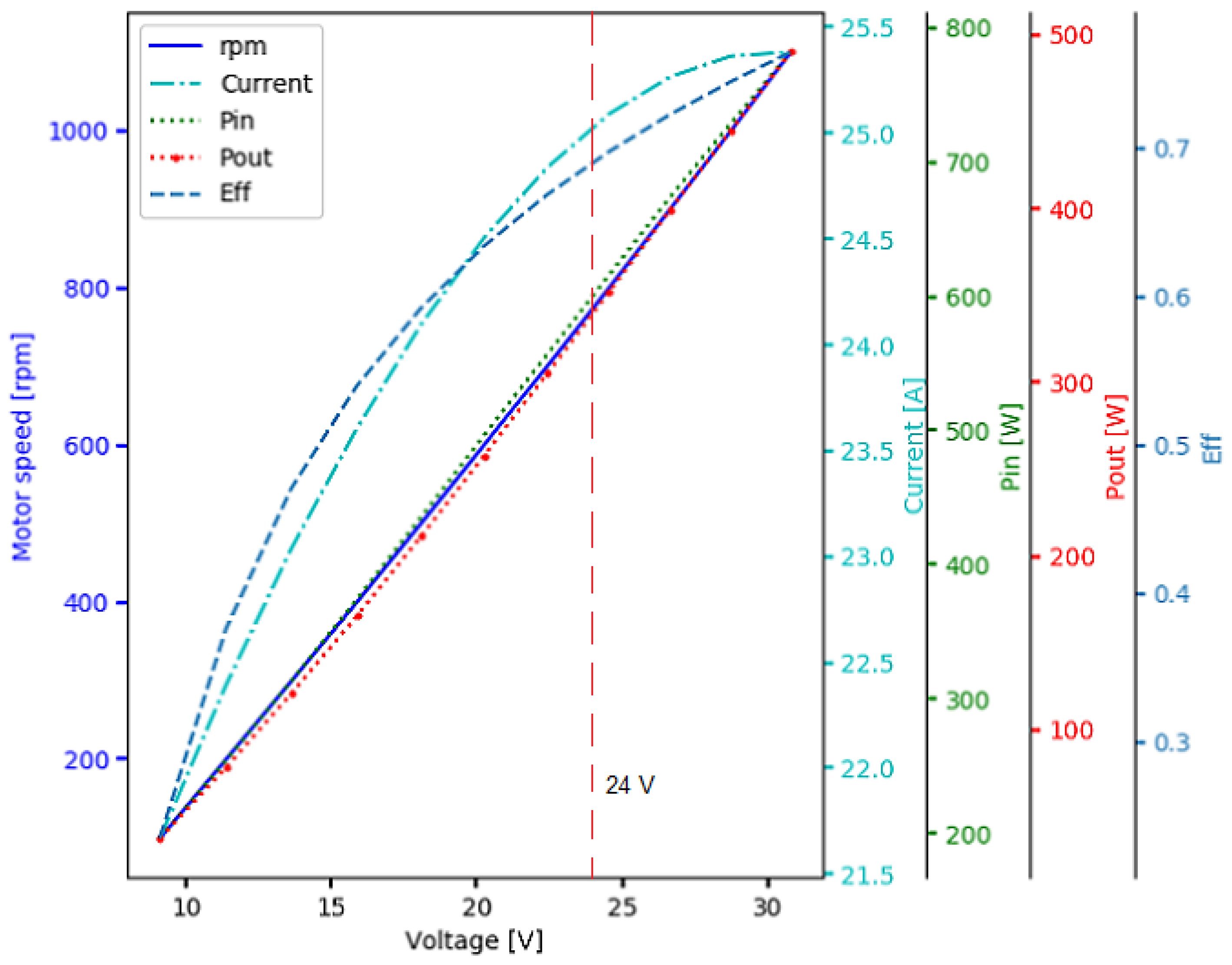
As the compensator will operate as a self-powered device [23], one of the constraints in the operation is to minimize the power consumption while achieving the targets for positioning at minimal error. The plot in Figure 14 shows the simulation results of running the compensator based on the data series of Figure 11. The result shows the estimated energy required to adjust the chain position. The load calculated as the translator and the connection line weights was estimated to be 100 kN. In general, the faster the compensator system is allowed to turn, the less energy is required for the operation and the higher voltage is needed to power the motor. However, the device was chosen to be powered by two 12-V, 100-Ah batteries connected in series. Figure 15 shows the estimated voltage required to turn the motor at the designated rpm (left, vertical axis). From this figure, it can be concluded that the motor should be operated at the highest battery capacity of 24 V to turn the motor at the highest speed (800 rpm) and with high efficiency. With reference to Figure 14, it is noticeable that at 800 rpm, the energy required to operate the system is already at a minimum.
3.3. Adaptation to Wave Hub
The analysis of the estimated power consumption of the compensation system at Wave Hub is shown in Figure 16. The simulation compared the control strategy for four different time intervals between each compensating operation. 15-, 30-, 60-, and 120-min intervals were chosen for the study. In each case, the compensator will start to compensate until it reaches the calculated position (extrapolated) of the sea level. Table 3 tabulates the RMSE values as the performance evaluation of the compensator position; see the dashed line (labeled with “error” and “compensator interval”) in Figure 13b. The power consumptions and the RMSEs were analyzed for a period of one year (2017–2018). The result shows that the power consumption of the system when it runs at its full capacity of 24 V, which corresponds to 800 rpm (see Figure 15), was around 600–640 Wh. As the batteries were rated 100 Ah, 24 V, the system should last for three days without charging.
4. Discussion
Due to the high turn ratio of the gearbox (1:4758), one pulse per revolution of the motor is enough to get high accuracy on the chain position. As the number of the revolution of the shaft is high, the encoder suitable for this application is the incremental type, with the ability to restore the last position (saved in Raspberry Pi) after a reset. Moreover, the custom protocol as it is currently designed has facilitated the system well: the slow encoder output frequency, yet high accuracy (due to the high turn ratio), and the mechanism of detecting turn direction (CCW/CW) on every encoder’s pulse.
The highest pulling force tested in the lab was 104 kN. The result plotted in Figure 8 shows that the force measurements from the torque sensor were reliable. Adjustments were made to calibrate and remove the sensor offset. In order to test the system in real time, we removed the load (springs) for safety reasons. Moreover, the main goal for the positioning test was to evaluate the control strategy and communication for a long duration, from the collection of sea level data to moving the chain to the new, desired position. Due to the slow change in sea level at the measurement station of Brofjorden, the lag between data collection and the adjustment of the connection line can be neglected.
The approach of utilizing a series of 10 h of sea level information to predict the next two hours was based on the understanding that changes in sea level follow a semi-diurnal trend with an M2 constituent period of about 12 h and 25 min. Based on this, the previous 10 h of data were used to extrapolate the data points of the next two hours and to get rid of the effects due to low-frequency variations. This method was also used to simplify the calculations. The analysis of the RMSE values calculated over 19 days of data led to an error between predictions and observations of 7.4 cm (see Table 2). This RMSE value was found to be lower than the RMSE of short- and long-forecast data; hence, it was selected for calculating the new desired position of the chain.
Attempts to lift a heavy load dynamically have been done in [16], but only loads of up to 35 kN could be lifted for safety reasons in the lab environment. However, there were many uncertainties due to the configuration of the setup and the accuracy of the measurements. Our test improved the understanding of the system and the DC motor behavior based on the input signal. It also contributed to dimensioning the power supply system and evaluating power consumption. From the plot in Figure 14, it can be seen that the faster the motor, the less total energy is required for the operation. However, this will be smoothed out because of the reduced efficiency of the motor at high speed (and current). Looking at the behavior of the curve of total energy consumption, we decided that the motor should run at a steady state of 800 rpm. This would correspond to a standard battery supply of 24 V. The relationship between the speed of the motor and the voltage supplied is shown in Figure 15.
The result of the analysis of the speed and operating intervals for Wave Hub shows that the effect of the interval control on the power consumption was minimal. All intervals tested consumed roughly the same amounts of energy. One thing to consider in this respect is to put a limit on the interval (on/off time) so that the error of the compensator can be kept at a minimum to optimize the power production of the WEC. With reference to [12,24], the negative effects of the changes in tidal level on the power production were in general minimal when the variation in the tides were in the range of 0.2 m at Wave Hub. As can be inferred from Table 3, a time interval of 15 min (or shorter) was suitable to keep the error of the compensator and the sea level the whole time smaller than 0.2 m. However, the effect of the sea level change on the power production will also depend on the stroke length of the generator and the wave climate. At smaller wave heights, the negative effect of sea level change is minimal, and thus, the time interval for the compensator can be longer while maintaining the power production.
The input (sea level) to the system is currently obtained from the observatory-station’s sea level data available online from SMHI. This strategy can be robust considering it suits different types of WEC devices regardless of whether the WEC (or a wave farm) has its local sea level measurement. However, if a WEC has its position measurement installed, e.g., translator position in the generator, this position input can be used for a more accurate compensation (directly compensates for translator’s shift) compared to the measured (or forecast) data from observatory station, which is usually situated away from the wave farm.
5. Conclusions
A remotely-controlled sea level compensator for WECs was designed, built, and evaluated. The experiment was held in the lab with the input to the system being the observed sea levels at Brofjorden observatory station, collected online from SMHI. Additionally, offline sea level data were analyzed, and the device operations were simulated to evaluate the control strategy and the compensator behavior for the operation of the device in a higher tidal range, e.g., Wave Hub.
The experimental tests in the lab have shown that the integration of the control and the communication systems worked reasonably well. As a self-powered device, the system had the right dimensions to be capable of lifting the load with minimal energy, as demonstrated by the analysis of the power consumption. The daily power consumption was not affected by the time interval selected for the operation, at least for the time period simulated. However, the power consumption was more influenced by the permitted error variations (RMSE) of the compensator for optimal power production on the side of the main WEC: the larger the RMSE for the compensator positioning resulted in lower power production at the main WEC. For Wave Hub to maximize the power production, the time interval between the adjustments should not be longer than 15 min at a motor speed of approximately 800 rpm.
Author Contributions
M.N.A. contributed to the development of the device, designing the experimental setup and control system, analyzing the result, and writing the article. V.C. contributed to the experimental setup and analyzing the result. J.A. contributing technical support. R.W. supervised the work and provided financial support. All co-authors participated in writing the article.
Funding
This research was funded by Swedish Energy Agency grant number 2016-002062.
Acknowledgments
M.N.A. is funded by the Ministry of Education of Malaysia. J.J. Perez-Loya and D. Salar are acknowledged for their help with the experimental setup. Thanks go to the Swedish Energy Agency and Ångpanneföreningen for their financial support.
Conflicts of Interest
The authors declare no conflict of interest.
Abbreviations
The following abbreviations are used in this manuscript:
| AMQP | Advanced Message Queuing Protocol |
| BODC | British Oceanographic Data Centre |
| CCW | Counter-clockwise |
| CW | Clockwise |
| DC | Direct current |
| DWR | Draw wire sensor |
| GUI | Graphical user interface |
| IoT | Internet of Things |
| M2 | Principle lunar semi-diurnal tide |
| MQ | Messaging queue |
| PV | Photovoltaic |
| RMSE | Root mean square error |
| SMHI | Swedish Meteorological and Hydrological Institute |
| UU | Uppsala University |
| VPN | Virtual private network |
| WEC | Wave energy converter |
References
- Engström, J. Hydrodynamic Modelling for a Point Absorbing Wave Energy Converter. Ph.D. Thesis, Electricity, Department of Engineering Sciences, Technology, Disciplinary Domain of Science and Technology, Uppsala University, Uppsala, Sweden, 2011. [Google Scholar]
- Yavuz, H.; McCabe, A.; Aggidis, G.; Widden, M.B. Calculation of the performance of resonant wave energy converters in real seas. Proc. Inst. Mech. Eng. Part M 2006, 220, 117–128. [Google Scholar] [CrossRef]
- Eriksson, M.; Isberg, J.; Leijon, M. Hydrodynamic modelling of a direct drive wave energy converter. Int. J. Eng. Sci. 2005, 43, 1377–1387. [Google Scholar] [CrossRef]
- Bozzi, S.; Miquel, A.; Antonini, A.; Passoni, G.; Archetti, R. Modeling of a Point Absorber for Energy Conversion in Italian Seas. Energies 2013, 6, 3033–3051. [Google Scholar] [CrossRef] [Green Version]
- Lejerskog, E.; Boström, C.; Hai, L.; Waters, R.; Leijon, M. Experimental results on power absorption from a wave energy converter at the Lysekil wave energy research site. Renew. Energy 2015, 77, 9–14. [Google Scholar] [CrossRef]
- Liang, C.; Ai, J.; Zuo, L. Design, fabrication, simulation and testing of an ocean wave energy converter with mechanical motion rectifier. Ocean. Eng. 2017, 136, 190–200. [Google Scholar] [CrossRef]
- Waters, R.; Stålberg, M.; Danielsson, O.; Svensson, O.; Gustafsson, S.; Strömstedt, E.; Eriksson, M.; Sundberg, J.; Leijon, M. Experimental results from sea trials of an offshore wave energy system. Appl. Phys. Lett. 2007, 90, 034105. [Google Scholar] [CrossRef]
- Rusu, E. Evaluation of the Wave Energy Conversion Efficiency in Various Coastal Environments. Energies 2014, 7, 4002–4018. [Google Scholar] [CrossRef] [Green Version]
- Belibassakis, K.; Bonovas, M.; Rusu, E. A Novel Method for Estimating Wave Energy Converter Performance in Variable Bathymetry Regions and Applications. Energies 2018, 11, 2092. [Google Scholar] [CrossRef]
- Silva, D.; Rusu, E.; Soares, C. Evaluation of Various Technologies for Wave Energy Conversion in the Portuguese Nearshore. Energies 2013, 6, 1344–1364. [Google Scholar] [CrossRef]
- Castellucci, V.; Abrahamsson, J.; Kamf, T.; Waters, R. Nearshore Tests of the Tidal Compensation System for Point-Absorbing Wave Energy Converters. Energies 2015, 8, 3272–3291. [Google Scholar] [CrossRef] [Green Version]
- Castellucci, V.; Eriksson, M.; Waters, R. Impact of Tidal Level Variations on Wave Energy Absorption at Wave Hub. Energies 2016, 9, 843. [Google Scholar] [CrossRef]
- British Oceanographic Data Centre. Available online: https://www.bodc.ac.uk (accessed on 11 May 2016).
- Bonfiglioli. Available online: http://www.bonfiglioli.com (accessed on 21 February 2017).
- Swedish Meteorological and Hydrological Institute. Available online: https://www.smhi.se (accessed on 8 March 2018).
- Ayob, M.N.; Castellucci, V.; Abrahamsson, J.; Svensson, O.; Waters, R. Control strategy for a tidal compensation system for wave energy converter device. In Proceedings of the 28th International Offshore and Polar Engineering Conference, Sapporo, Japan, 10–15 June 2018; pp. 808–812. [Google Scholar]
- scipy.org. Available online: https://docs.scipy.org/doc/scipy/reference/generated/scipy.optimize.curve_fit.html (accessed on 9 April 2019).
- CloudAMQP. Available online: https://www.cloudamqp.com (accessed on 9 April 2019).
- ARDUINO MEGA 2560. Available online: https://store.arduino.cc/arduino-mega-2560-rev3 (accessed on 24 January 2018).
- Lopez-Vargas, A.; Fuentes, M.; Vivar, M. IoT Application for Real-Time Monitoring of Solar Home Systems Based on Arduino™ With 3G Connectivity. IEEE Sensors J. 2019, 19, 679–691. [Google Scholar] [CrossRef]
- Paredes-Parra, J.M.; García-Sánchez, A.J.; Mateo-Aroca, A.; Molina-Garcia, A. An Alternative Internet-of-Things Solution Based on LoRa for PV Power Plants: Data Monitoring and Management. Energies 2019, 12, 881. [Google Scholar] [CrossRef]
- NCTE Torque sensor. Available online: https://www.elfa.se/Web/Downloads/_t/ds/serie2000_eng_tds.pdf (accessed on 9 April 2019).
- Ayob, M.; Castellucci, V.; Göteman, M.; Widén, J.; Abrahamsson, J.; Engström, J.; Waters, R. Small-Scale Renewable Energy Converters for Battery Charging. J. Mar. Sci. Eng. 2018, 6, 26. [Google Scholar] [CrossRef]
- Tyrberg, S.; Waters, R.; Leijon, M. Wave Power Absorption as a Function of Water Level and Wave Height: Theory and Experiment. IEEE J. Ocean. Eng. 2010, 35, 558–564. [Google Scholar] [CrossRef] [Green Version]
Figure 1.
Control flow for the sea level compensation system. The part of the system surrounded by the blue dashed line is shown in Figure 2.
Figure 1.
Control flow for the sea level compensation system. The part of the system surrounded by the blue dashed line is shown in Figure 2.

Figure 2.
(a) Schematic of the compensator system [16]. (b) Electrical connection installed in the metal cabinet.
Figure 2.
(a) Schematic of the compensator system [16]. (b) Electrical connection installed in the metal cabinet.

Figure 3.
The forecasted and the observed sea level for a period of 10 days (long forecast), 7 days (short forecast), and 5 days (observation) recorded at the Brofjorden measurement station in October 2018.
Figure 3.
The forecasted and the observed sea level for a period of 10 days (long forecast), 7 days (short forecast), and 5 days (observation) recorded at the Brofjorden measurement station in October 2018.

Figure 4.
Illustration of 2-h extrapolation based on a sinusoidal fitting for 10 h of observed sea levels.
Figure 4.
Illustration of 2-h extrapolation based on a sinusoidal fitting for 10 h of observed sea levels.

Figure 5.
(a) Torque sensor with the coupler attached to the shaft. (b) Two permanent magnets attached to the coupler, connecting the shaft of the torque sensor to the gearbox. A Hall effect sensor acts as a switching device, which turns on/off when facing the magnets of different poles.
Figure 5.
(a) Torque sensor with the coupler attached to the shaft. (b) Two permanent magnets attached to the coupler, connecting the shaft of the torque sensor to the gearbox. A Hall effect sensor acts as a switching device, which turns on/off when facing the magnets of different poles.

Figure 6.
Recorded encoder output. (a) Motor clockwise (CW) rotation. (b) Motor counter-clockwise (CCW) rotation. The output from the sensor always gives approximately a 25% or 75% duty cycle from the CW or CCW regardless of the speed.
Figure 6.
Recorded encoder output. (a) Motor clockwise (CW) rotation. (b) Motor counter-clockwise (CCW) rotation. The output from the sensor always gives approximately a 25% or 75% duty cycle from the CW or CCW regardless of the speed.

Figure 7.
(a) The compensator system with the parts labeled in the image. (b) The steel chain pulls the load cell.
Figure 7.
(a) The compensator system with the parts labeled in the image. (b) The steel chain pulls the load cell.

Figure 8.
Result from the torque sensor calibration test.

Figure 9.
The torque measured at the output shaft of the DC motor with respect to the current fed in.
Figure 9.
The torque measured at the output shaft of the DC motor with respect to the current fed in.

Figure 10.
The relationship between the power fed in and the power put out, as measured from the DC motor, to determine the other losses after the copper losses () have been accounted for.
Figure 10.
The relationship between the power fed in and the power put out, as measured from the DC motor, to determine the other losses after the copper losses () have been accounted for.

Figure 11.
(a) Two-hour prediction from the observational data compared to long- and short-forecast data in October 2018 (available from SMHI). (b) A zoom in of two days of data.
Figure 11.
(a) Two-hour prediction from the observational data compared to long- and short-forecast data in October 2018 (available from SMHI). (b) A zoom in of two days of data.

Figure 12.
(a) Sea level at Brofjorden. (b) GUI for the control settings.

Figure 13.
(a) Experimental results from a positioning test of the chain in October 2018. (b) Zoom out of the area marked by the dotted rectangle in (a).
Figure 13.
(a) Experimental results from a positioning test of the chain in October 2018. (b) Zoom out of the area marked by the dotted rectangle in (a).

Figure 14.
The analysis of the energy required by the motor and the brake and the standby power for the 19-day period analyzed (as in Figure 11). The dashed blue line shows the total time required to turn the motor. The green line shows the energy required to release the brake when the motor turns. The red line shows the standby energy, which is approximately the same throughout the test period.

Figure 15.
The motor behavior with respect to speed and its corresponding parameters when the motor is powered with different voltage levels and the applied load is set to 100 kN. The red dashed line shows the level of the nominal voltage supplied by the batteries.
Figure 15.
The motor behavior with respect to speed and its corresponding parameters when the motor is powered with different voltage levels and the applied load is set to 100 kN. The red dashed line shows the level of the nominal voltage supplied by the batteries.

Figure 16.
Estimated energy consumption for 24 h with different compensating time intervals for the operation at Wave Hub.
Figure 16.
Estimated energy consumption for 24 h with different compensating time intervals for the operation at Wave Hub.


Table 1.
Information from the encoder measurements.
| Figure 6 | Duty Cycle | Direction: Connection Line | Motor rpm | Speed at Chain (mm/s) rpm × | Linear Position Corresponding to One Motor Revolution |
|---|---|---|---|---|---|
| (a) | 25% | CW: release | 579 | 2.0 | 0.2 mm |
| (b) | 75% | CCW: retract | 600 | 2.1 | 0.2 mm |
Table 2.
Root mean squared error (RMSE).
| Data Type | 2-h Extrapolation | Short Forecast | Long Forecast |
|---|---|---|---|
| RMSE (cm) | 7.4 | 8.1 | 9.9 |
Time analysis: 3 October 2018, 1100–22 October 2018, 0900 (19 days).
Table 3.
RMSE between compensator position and sea level for different control strategies.
| Interval Time (minutes) | RMSE (cm) |
|---|---|
| 15 | 17 |
| 30 | 34 |
| 60 | 67 |
| 120 | 130 |
© 2019 by the authors. Licensee MDPI, Basel, Switzerland. This article is an open access article distributed under the terms and conditions of the Creative Commons Attribution (CC BY) license (http://creativecommons.org/licenses/by/4.0/).
Share and Cite
MDPI and ACS Style
Ayob, M.N.; Castellucci, V.; Abrahamsson, J.; Waters, R. A Remotely Controlled Sea Level Compensation System for Wave Energy Converters. Energies 2019, 12, 1946. https://doi.org/10.3390/en12101946
AMA Style
Ayob MN, Castellucci V, Abrahamsson J, Waters R. A Remotely Controlled Sea Level Compensation System for Wave Energy Converters. Energies. 2019; 12(10):1946. https://doi.org/10.3390/en12101946
Chicago/Turabian StyleAyob, Mohd Nasir, Valeria Castellucci, Johan Abrahamsson, and Rafael Waters. 2019. "A Remotely Controlled Sea Level Compensation System for Wave Energy Converters" Energies 12, no. 10: 1946. https://doi.org/10.3390/en12101946
Note that from the first issue of 2016, this journal uses article numbers instead of page numbers. See further details here.