Experimental and Theoretical Study on Dynamic Hydraulic Fracture
by
Jingnan Dong
1,2,3, 
Mian Chen
1,2,4,*,
Yuwei Li
4,
Shiyong Wang
1,2,
Chao Zeng
5 and
Musharraf Zaman
3 1
State Key Laboratory of Petroleum Resources and Prospecting, Beijing 102249, China
2
College of Petroleum Engineering, China University of Petroleum, Beijing 102249, China
3
Mewbourne School of Petroleum and Geological Engineering, University of Oklahoma, Norman, OK 73019, USA
4
Institute of Unconventional Oil & Gas, Northeast Petroleum University, Daqing 163318, China
5
Department of Civil, Architectural and Environmental Engineering, Missouri University of Sciences and Technology, Rolla, MO 65409, USA
*
Author to whom correspondence should be addressed.
Energies 2019, 12(3), 397; https://doi.org/10.3390/en12030397
Submission received: 7 January 2019
/
Revised: 23 January 2019
/
Accepted: 24 January 2019
/
Published: 27 January 2019
(This article belongs to the Special Issue Mathematical Modeling of Fluid Flow and Heat Transfer in Petroleum Industries and Geothermal Applications)
Abstract
:Hydraulic fracturing is vital in the stimulation of oil and gas reservoirs, whereas the dynamic process during hydraulic fracturing is still unclear due to the difficulty in capturing the behavior of both fluid and fracture in the transient process. For the first time, the direct observations and theoretical analyses of the relationship between the crack tip and the fluid front in a dynamic hydraulic fracture are presented. A laboratory-scale hydraulic fracturing device is built. The momentum-balance equation of the fracturing fluid is established and numerically solved. The theoretical predictions conform well to the directly observed relationship between the crack tip and the fluid front. The kinetic energy of the fluid occupies over half of the total input energy. Using dimensionless analyses, the existence of equilibrium state of the driving fluid in this dynamic system is theoretically established and experimentally verified. The dimensionless separation criterion of the crack tip and the fluid front in the dynamic situation is established and conforms well to the experimental data. The dynamic analyses show that the separation of crack tip and fluid front is dominated by the crack profile and the equilibrium fluid velocity. This study provides a better understanding of the dynamic hydraulic fracture.
1. Introduction
Hydraulic fracturing is an inherently unstable process. Even the controlled and overall stable hydraulic fracture propagation is unstable at the small scale [1]. Most previous studies on hydraulic fracture are based on the quasi-static treatment of the fracturing fluid and the inertial force of the fluid is neglected [2,3,4]. The dynamic situation is fundamentally different from the quasi-static simulation. For example, it has been shown that in the quasi-static fluid-driven crack, the fluid front has a relationship of with time in a quasi-static situation where the inertial force is neglected and viscosity dominates the fluid behavior [4]. According to the dynamic simulation considered herein, the velocity of fluid front advancement is approximately constant in a propagating crack traveling at a constant speed. A recent numerical study [5] on a dynamic hydraulic fracture taking the inertia effect into account has shown that the hydraulic fracture propagates in a stepwise manner with fluid pressure oscillations. The stepwise propagation of the crack and the pressure oscillations indicate that the fluid inertia plays an important role in the dynamic fracturing, especially within the short time period right after the crack initiation.
The most widely known phenomenon of the relationship between crack tip and fluid front is the “lag region (dry zone)”. The lag region is the space between the crack tip and fluid front. Under some specific conditions [4], the lag region could be considered infinitely small, exerting no influence on the fracturing behavior. There are also studies [6,7,8,9] showing that although the length of lag zone is indeed very small, its effect on fracture geometry cannot be ignored. For example, Bunger [10] considered the lag region to be filled by vapor from the fluid at a pressure that is negligibly small compared to the characteristic pressure in the fracturing process. The existence of the lag region induces another characteristic length besides the crack length. Previous studies related to the lag region have all been based on static or quasi-static assumptions of fluid behavior. The present study provides both experimental and theoretical insights on the lag region in dynamic situation.
Recently, the dynamic hydraulic fracturing was numerically investigated by Khoei et al. [11] and Kostov et al. [12] using Extended Finite Element Method (XFEM). To the authors’ knowledge, no previous studies have reported direct observations of the real dynamic process of hydraulic fracture. In terms of experimental observations, we have limited knowledge on the effect of inertia after the initiation of the hydraulic fracture. In most previous experimental studies [10,13,14,15,16,17,18,19,20,21,22], the time spans of the experiments were on the scale of seconds and the data acquisition interval was too large to capture the dynamic response within seconds. Moreover, the data from the oil field [23] were on a larger time scale making dynamic analysis intractable. In this paper it demonstrates that the inertial force of the fluid plays an important role in dynamic hydraulic fracture. This is achieved by direct observations and theoretical analyses of the relationship between the crack tip and the fluid front in dynamic hydraulic fracture. The dimensionless separation criterion of the crack tip and the fluid front is also established to provide a guideline of distinguishing dynamic hydraulic fracture from the quasi-static fluid-driven fracture in numerical simulations.
In order to describe the transient motion of the fluid in the fracture, the momentum balance equation regarding the fracturing fluid is established. The treatment generally follows the approach by Bosanquet [24]. A proper treatment of the crack profile is important to the dynamic analyses. The most well-known crack tip profile is the parabola (Linear Elastic Fracture Mechanics) described as , where is the crack opening and is the distance from the crack tip. Recent studies also showed that the hydraulic fracture had a profile of (zero-toughness situation) in the near tip region [25], and it transitioned to the form of away from the near-tip region [26,27,28] and finally it became after the crack attained blade-like geometry (Perkins–Kern–Nordgren model [29,30]). Thus, without loss of generality, the crack profile of is assumed in this study.
In this paper, a laboratory-scale hydraulic fracturing device is built to create dynamic Mode I hydraulic fracture (HF) in a double-cantilever-beam (DCB) shaped Polymethyl methacrylate (PMMA) specimens. The analytic solution of the beam deflection and stress intensity factor (SIF) are derived. To validate the calculated SIF, the analytic SIF is compared with the existing theoretical study. Then, the relationship between crack tip and fluid front in dynamic HF is investigated. The momentum balance equation of dynamic flow is established. Numerical results by solving this equation are compared with the pertinent experimental results. The corresponding energy form of equations are considered. The existence of equilibrium state is predicted theoretically and experimentally verified. The influence of crack profile is taken into consideration. A dimensionless factor is proposed as the dimensionless separation criterion to study the separation of the crack tip and the fluid front, as well as the existence of equilibrium state. The validity of is verified by the experimental results.
2. Experimental Setup and Verification
The purpose of this section is to provide an overview of the experimental setup, the theoretical and experimental verification of this device and the tests performed. Two types of tests are performed in this study. The first focuses on the experimental verification of SIF using a combination of the Digital Image Correlation (DIC) method and the Williams’ series. An optical microscope is used to obtain the image. The second type captures the relationship between crack tip and fluid front in the dynamically propagating crack. A high-speed camera is used for this purpose.
2.1. Experimental Setup
In this study, a laboratory-scale hydraulic fracture device, based on the DCB test, is designed and built. In order to acquire photographs using both optical microscope and high-speed camera, two transparent and thick PMMA boards are machined into certain shape and used as the frame structure. As a result of the difficulty in sealing the top of the specimen against fluid leaks, a relatively soft silicone ring is used as the sealing material. To seal the specimen surface, two U-shape silicone strips are placed on both sides of the specimen surface. As shown in Figure 1a, this design creates two narrow spaces filled with pressurized fracturing fluid on both sides of the specimen. Silicone seals offer great performance according to our experimental observations. In order to obtain a straight crack path, a small force parallel to the crack direction is applied to the DCB specimen. This small force not only ensures a straight crack path, but also makes the specimen squeeze the silicone ring against any fluid leaks. Care was taken to avoid applying a relatively large force that can lead to fluid leaks. The fluid is injected into the void between the two beams of the specimen. To capture the fluid front during the high-speed dynamic crack propagation, distilled water with a small amount of black ink is used as fracturing fluid. For tests conducted to verify the SIF value using an optical microscope, only distilled water is used as the fracturing fluid.
The PMMA specimens are commercial products having an elastic modulus of 2.6 GPa and a Poisson’s ratio of 0.33, evaluating using uniaxial compression test in a RTR-1500 tri-axial machine manufactured by GCTS. The details of the geometrical parameters are shown in Figure 1b. The thickness of the specimen is maintained at b = 5.0 mm ± 0.1 mm. Crack notch of different widths is studied. The width varied from intrinsically sharp to 2.0 mm. The intrinsically sharp crack is induced by Chevron notch, as shown in Figure 1c, with a length a = 35 mm ± 2 mm. The other notch widths (0.5 mm and 1.0 mm and 2.0 mm) with length a = 30 mm, are produced by laser cutting.
In order to create an ideal two-dimensional flow, a copper foil of 0.05 mm thickness (1% of the sample thickness) is pasted on each side of the specimen to avoid side flow of fracturing fluid to the crack tip. This experimental treatment ensures that the fracturing fluid is only supplied by the rear end of the fracture. According to our observations, the copper foil offers great performance in resisting the side flow from the specimen surface and it does not exert any influence on the fracturing behavior of the specimen.
In the tests herein, a RTR-1500 hydraulic system and a SCON controlling system from GCTS are used as the hydraulic system and the controlling system, respectively. A high-speed camera is used to capture the dynamic relationship of crack tip and fluid front. A typical data acquisition interval of 5 microseconds is used. A 2000 watt high-power light source and several high-power flashlights are used together to provide sufficient light for the camera for capturing images with a very small exposure time (about 4 microseconds). In this paper, the dynamic relationship between fluid front and crack tip is directly captured within 1 millisecond using a high-speed camera with a sampling rate of 200,000 Hz (sampling interval: 5 µs).
Tests are performed in a displacement (fluid volume) control mode. The injection rate is kept at 17.4 mL/min. The following data are collected: transient fluid pressure as a function of time (using the GCTS system), dynamic relationship of crack tip and fluid front (using high-speed camera) and full-field displacement (using optical microscope (OM)).
2.2. The Theoretical and Experimental Verification of Stress Intensity Factor (SIF)
2.2.1. Theoretical Verification
The deflection and SIF of HF-DCB specimen under hydraulic pressure are derived. Based on the Euler-Bernoulli beam theory and the Winkler foundation, Kanninen [31] derived the following closed-form analytic solution of the beam deflection of the DCB specimen under point load.
where,
All other parameters are shown in Figure 1b. Based on the point load solution shown above, the solution of the DCB specimen under uniformly distributed load, namely the solution of the HF-DCB specimen is derived. The analytic solution of beam deflection, the total strain energy stored in the HF-DCB specimen, the energy release rate and the SIF of the HF-DCB specimen are derived as follows:
where,
The details of the derivation are shown in Appendix A. The fluid volume between two beams is expressed as follows:
According to Equations (3) and (8), the total strain energy has the following relationship with volume: .
As commonly seen in DCB analyses, Equation (5) is very insensitive to c when , in which situation it reduces to the following:
The SIF is compared with the results by Fett [32] who derived the SIF under a distributed load using the boundary collocation method and the weight functions. According to his study, can be expressed as follows:
where is a constant and the weight function is given by
Thus, can be written as follows
A comparison between the Fett’s results (Equation (12)) and the analytic solution derived in this study (Equation (5)) is shown in Figure 2. It can be seen that the analytic results are in good agreement with the Fett’s results. It should be noted that the Fett’s results present a numerical fitting and are only applicable in the condition of . The analytic solution in Equation (5) provides a generalized analytic solution without this constraint of .
2.2.2. Experimental Verification
The theoretical SIF expressed in Equation (9) is experimentally verified using a combined method of DIC full-field displacement extraction and the fitting of Williams’ series. The crack tip position, Mode I and Mode II SIFs are unknown parameters in the fitting. This non-linear fitting is performed in the least square sense using a derivative-free Levenberg-Marquardt algorithm [33,34]. A comparison between theoretical SIFs and experimental SIFs results under different values of is shown in Figure 3. The images for DIC analyses are taken by an Olympus optical microscope with a resolution of 1624 × 1236 pixels, and a pixel length of 8.09 µm. For better DIC identification, the specimen surface around crack tip is abraded by 800 grit sandpaper. All the fitting process generally follows the method by Yates [35]. The details of the fitting process are not shown here.
3. The Relationship Between the Crack Tip and the Fluid Front in Dynamic Hydraulic Fracture (HF)
3.1. Governing Equations
The two-dimensional dynamic flow in hydraulic fracture studied here can be approximated as dynamic flow along slowly-varying channels. The momentum-balance equation of the fracturing fluid between the slowly-varying plates under constant fracturing pressure is as follows [36,37]:
In this equation, the coordinate system is established as show in Figure 4. is the position of the fluid front (not the same in beam deflection analyses), the first term on the left side of the equation is the inertial resistance, is the total momentum of the fluid, the second term stands for the drag force induced by viscosity, the third term is the resistance induced by the slowly-varying flanks of the crack, and is the total driving force. It may be worth noting that is also a function of . This momentum balance equation has the following expanded form:
where is the crack opening width as a function of time and fluid front position x.
The first term on the left side of Equation (14) is the time derivative of the total momentum of the fluid in the propagating crack:
where and (volume conservation) as shown in Figure 4. The second term on the left side of Equation (14) is the viscous force:
where .
The third term is the horizontal component of the resistance applied by the crack flanks:
Strictly speaking, the derivation of the third term requires an explicit , which can only be obtained by solving Equation (14). This makes Equation (14) implicit. Here the pressure distribution for the calculation of the third term is assumed to have the following linear form:
This first order assumption ensures the pressure at the fluid front is zero and is at the injection point. The influence of the crack-flank resistance term is discussed later in this paper.
The derivation of Equation (14) contains the following assumptions. Firstly, the fluid is assumed to fully fill the crack in the rear of fluid front. Secondly, the fluid front is assumed to have a flat profile. The velocity of the fluid at point is considered as the mean velocity at any cross section.
It can be inferred that the theoretical fluid front as a function of time is strongly influenced by the time-dependent crack profile, . The determination of is also where the difficulty resides in. According to our experimental results of crack tip velocity, for some of the tests, before first arrest of the crack, the hydraulic crack in DCB specimen roughly propagates at a constant velocity. Thus, the constant-velocity approximations are made in sample #15 and sample #16. As for sample #12 and sample #14, nine-order polynomial fitting is used to fit the crack tip position as a function of time. It should be noted that if the details of the curve are not omitted, five-order polynomial fitting is suggested as the fitting becomes sensitive to the error when the order increases. In the case we investigate here, the crack profile in the DCB specimen is approximated by linear approximation. The comparison between approximation of the crack profile and the theoretical quasi-static crack profile derived by Equation (A7) is shown in Figure 5. As shown, the linear crack profile provides a good approximation in the range of crack length we investigated here.
According to the approximations of linear crack profile, the can be expressed as:
is a constant in all the tests and has a non-dimensional value of . means the slope of the linear crack profile and is derived by fitting the theoretical quasi-static crack profile as shown in Figure 5. The theoretical quasi-static crack profile is obtained by substituting Equation (5) into Equation (A7) and eliminating . And the value of is set as the arrest toughness (1.0 , regular dry DCB tests). In this way is obtained.
has the following form under the approximation of constant-velocity crack.
In the nine-order polynomial fitting of the crack tip position, is expressed as:
Substituting Equation (19) into Equation (14) we have the following differential equation:
Equation (22) is a general equation for linear-profile crack. After substituting Equations (20) and (21) into Equation (22) separately, Equation (22) is numerically solved on MATLAB using “ode45”. The initial values of , and and are assigned a small positive value (typically ) because Equation (22) is singular at and . All the experimental and numerical results are shown in Figure 6 and Figure 7.
3.2. Energy Conservation in the Dynamic Process
The energy conservation of the fluid within the crack is investigated here. The major energy terms taking part in the energy conservation regarding the dynamic fluid flow include the input energy , the kinetic energy of the fluid , the energy dissipated by viscosity , and the work done by the fluid on the crack flanks . These terms as a function of time can be derived via the time integral of the rate of these energy terms, which are shown as follows:
The rate of energy dissipated by viscosity is calculated by visco-friction between the crack and fluid. The rate of work done on the crack flank involves the calculation of the force component on the direction of crack propagation.
The conservation of energy should be satisfied:
which can be written,
In the following section, the energy conservation is verified. After solving Equation (22), the total input energy as a function of time is compared with the total energy consumed by the fluid .
3.3. Comparison between Experimental and Theoretical Results
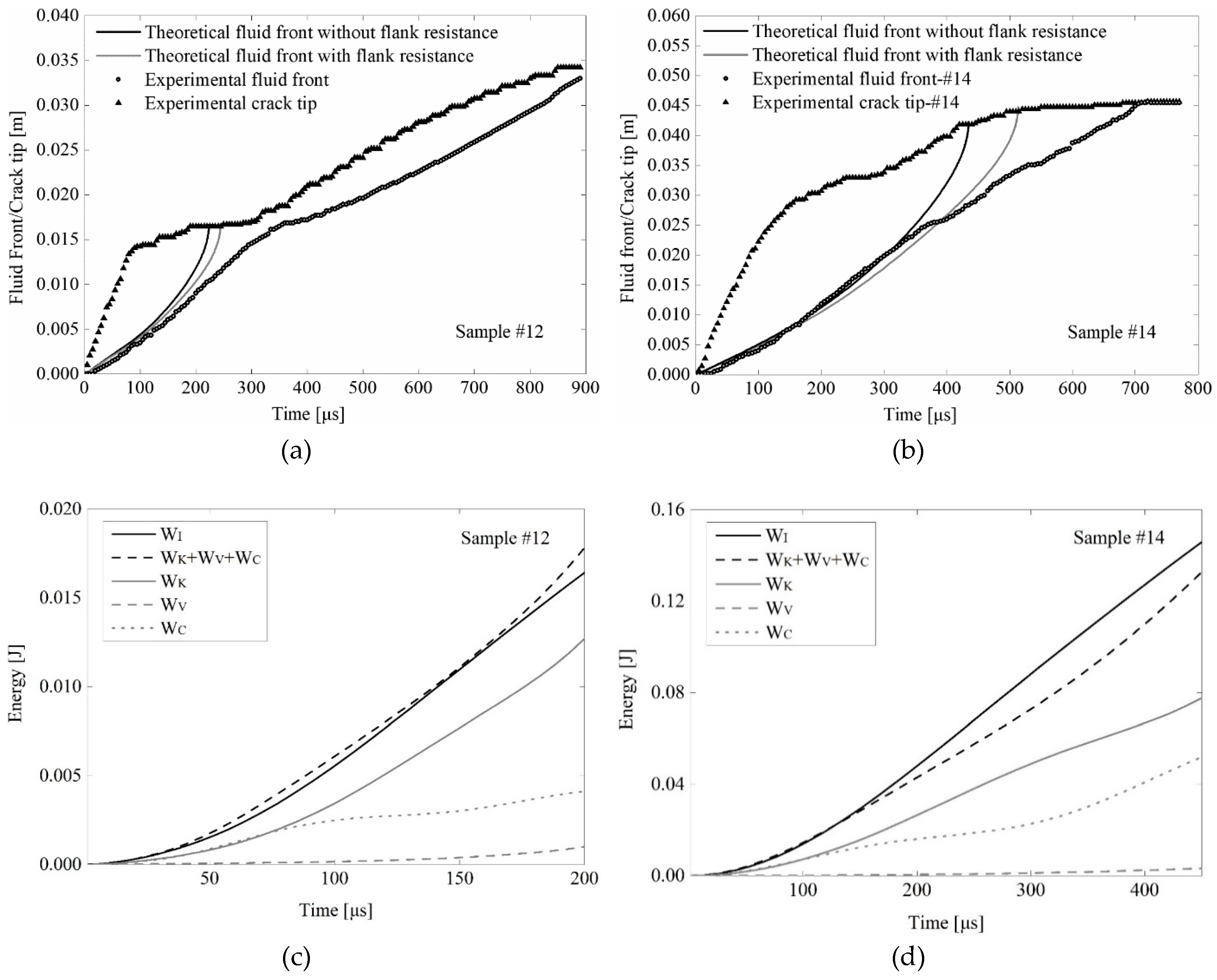
All the detailed data of the samples are shown in Table 1. The fracturing fluid is water with black ink. Because the viscosity of black ink is only slightly larger than the viscosity of water, the viscosity for calculation is set as , which is the viscosity of water at 25 degrees centigrade. Figure 6 and Figure 7 show the typical experimental and theoretical results of the dynamic process. The positions of the crack tip and fluid front are recorded frame by frame. As it can be seen in Figure 6a,b and Figure 7a,b, the theoretical dynamic fluid fronts are in good agreement with the experimental results. Both experimental results and numerical results show that during the dynamic propagation of the hydraulic fracture, the fluid front separates with the crack tip and has a different velocity compared to the crack. Before the fluid front approaches the crack tip, the results of the calculation with and without the crack-flank resistance term provide similar results. However, when the fluid front approaches the crack tip, the calculation with that term provides a much better result. It is because when approaching the crack tip, the fluid occupies most of the crack, and the horizontal component of the force applied by the crack flanks increases to an important part of the total resistance. The results indicate that when the fluid occupies most of the crack, the crack-flank resistant force is not negligible in a dynamic calculation.
As for the energy terms, in most of the time during propagation, the total input energy is almost the same as the total energy consumed by the fluid as shown in Figure 6c,d and Figure 7c,d. This is a good verification of the first-order approximation of pressure distribution. As can be seen, the viscosity energy is only a very small part of the total input energy. The kinetic energy of the fluid and the work done on the crack flank takes up most of the energy during the dynamic process. The results show that the value of has a positive relationship with the velocity of the crack tip. When the crack arrests, the stops to increase and the starts to decrease. This result is predicted by Equation (8), which involves the crack tip velocity. Overall, the kinetic energy of the fluid takes up over half of the total input energy during this process. When the crack slows down or is arrested, this ratio further increases. The and the share the rest of the input energy.
Recent numerical simulation [5] showed that the dynamic fracturing (in 1 millisecond) is not smooth or continuous but was a distinct stepwise process concomitant with fluid pressure oscillations. The experimental results here provide a direct evidence for the stepwise propagation of the crack in the dynamic situation. As it can be seen, the crack is prone to re-initiation when the fluid front approaches the crack tip. The crack speed of the re-initiation is higher than the fluid velocity, and the crack arrests before the fluid front approaches again. The experimental and theoretical results of crack tip and fluid front also agree with the existing studies [38,39,40].
Despite that the numerical results provided by solving Equation (22) are in good agreement with the experimental results, there are still problems that need further investigation. According to our numerical results, the fluid front allowing for the first-order approximation of the crack-flank resistance predict an extremely high fluid velocity when the fluid front further approaches the crack tip. It is not clear whether the behavior at such high speed is real or is simply an artifact of the model. Interestingly, the experimental results seem to provide some evidence of this high-speed phenomenon. Figure 8 shows the dynamic images of sample #12, which shares the same time coordinate with the data in Figure 6a. As can be seen, the fluid front becomes unstable after 0.235 milliseconds. This may result from the high speed of the fluid, which leads to turbulence. The data of the fluid front position in Figure 6a is not sampled at the very front of the unstable fluid after 0.235 milliseconds, as a result of which the velocity seems to be moderate when approaching the crack tip. If the very front of fluid is regarded as the fluid front, there will be the high speed of the fluid when approaching the crack tip. It should be noted that when the fluid front gets close to the crack tip, which is beyond the scope of this study, all the kinetic energy will turn into the work done on the crack flanks in the way of possible high fluid pressure. This may provide an explanation for the phenomenon that every time the fluid front approaches the crack tip, the crack starts to propagate. This phenomenon is seen in all the tests. Previous research by Rubin [41] showed that in the case of a saturated permeable media, the cavity between crack tip and fluid front was either filled with the vapor of the fracturing fluid, with a nearly constant vapor pressure in the case of an impermeable medium, or the pore-fluid infiltrated from the surrounding domain.
As can be seen, the crack tip shown in Figure 8 is vague. However, it is clear and readily identifiable in the video version in the Supplementary Materials.
3.4. Will the Fluid Front Catch Up with a Propagating Crack?
Now let us turn our attention to the separation of the fluid front and the crack tip during the dynamic process, namely the existence of the lag region. The main purpose of this section is to determine whether the fluid front and the crack tip share the same front or not after initiation, and to investigate the existence of the “equilibrium state” which indicates that the fluid front will travel at a constant velocity shortly after the initiation of the crack. Earlier discussion has already shown that the momentum-balance equation of the fracturing fluid between the linearly-slowly-varying plates can be expressed by Equation (14). It should be noted that the linear profile assumption is only valid in the crack of HF-DCB specimen. In the following analyses, a more generalized-form crack profile is investigated:
where is a positive real number. The coordinate is the same as the one shown in Figure 4. Equation (29) describes a more generalized profile of the crack propagating at a constant velocity. Using the first order approximation of crack-flank resistance, the governing equation can be written in the following form by substituting Equations (29) and (18) into Equation (14):
After the integral, Equation (30) becomes
Equation (31) can be written in the following dimensionless form:
where , the dimensionless instantaneous velocity of the fluid front; , the dimensionless secant velocity of the fluid front; and . , and are the composed criteria and is the simple criterion.
This governing equation mathematically predicts a dimensionless velocity: “equilibrium fluid velocity ”. It indicates an equilibrium state where after a long period of time () the fluid front travels at a constant velocity , and will not catch up with the running crack tip. The equilibrium state can only be approached. After a long period of time (), for there to be an equilibrium state, the instantaneous velocity of the fluid front equals the secant velocity and both are time independent, which leads to . Also notice that for . This makes the terms on the right side of Equation (14) readily integrable. After the time integral of Equation (32) over the range from 0 to t and by taking , we have the following dimensionless equation:
When , for there to be an equilibrium state, Equation (33) has to be satisfied. This equation can be utilized to examine the existence of the equilibrium state. It is easy to find that for an arbitrary n, Equation (33) first goes up then goes down when increases from 0 to 1. Thus, for Equation (33) to have a solution within the range of , there exists a critical , which can be expressed as . When <, the solution exists and the equilibrium state will finally be reached. After a long period of time, the fluid front will travel at a constant velocity that is slower than the crack tip and will not meet the crack tip. The equilibrium fluid velocity can be obtained by substituting a given set of and into Equation (33) and solving . In the case of >, the solution does not exist and there is not an equilibrium state for the system. The fluid front and the crack tip either keep sharing the same front right (low-viscosity situation) after the initiation of the crack or separate after initiation (viscosity-dominating situation). It should be noted that the relationship between and can only be numerically obtained as there is no explicit solution. It is worth noting that there is a maximum equilibrium fluid velocity when an equilibrium state exists. The value of can be solved by substituting a given and corresponding into Equation (33). The value of and maximum equilibrium fluid velocity as a function of are shown in Figure 9.
As can be seen in Figure 9, the maximum equilibrium fluid velocity cannot reach 1.0 over the range investigated. This means that when approaching the equilibrium state, despite the fluid length keeps occupying an invariable portion () of the crack length as time goes by, the crack tip and fluid front keep getting away from each other. It is also worth noting that the parameter , which characterizes the opening level of the crack, does not enter Equation (33). This means that the existence of equilibrium states is not related to the degree of the crack opening.
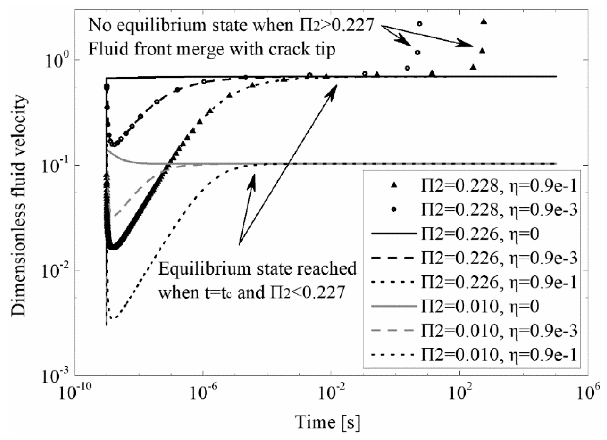
Figure 10 shows the numerical results of the dimensionless fluid velocity as a function of time under different and viscosity when . The numerical results verify the theoretical prediction of the existence of equilibrium state. Fluid fronts accelerate after the initiation of crack and gradually approach the equilibrium fluid velocity as long as . Once the becomes slightly larger than , there is no equilibrium state and the fluid front quickly rushes to the crack tip after a certain period of time . Provided that the stays the same and is smaller than , the fluid front finally travels at the same constant velocity after reaching the equilibrium state despite the difference of viscosity. High viscosity leads to a larger . It should be noted that the time needed for the fluid to approach the equilibrium state is actually related to . Higher leads to smaller . As can be seen in the earlier discussion, the lack of characteristic time indicates that can be regarded as the dimensional value carrying the dimension of time and enters the governing equation. The existence of is also seen in the experiments as shown in Figure 6a,b and Figure 7a,b: the fluid is relatively slow or even static in the first 5 microseconds to 25 microseconds. The fluid tends to accelerate from zero velocity to an approximately constant velocity after the initiation of the crack. The observed in the experiments varies from 5 microseconds to 25 microseconds.
Figure 11a shows the results of numerical (by solving Equation (30) using MATLAB “ode45”) and theoretical (by solving Equation (33)) equilibrium fluid velocity as a function of . As can be seen, the numerical solution and theoretical prediction are in consistent with each other. The numerical equilibrium fluid velocities are precisely predicted by Equation (33). The curves are much the same and are nearly linear in the range of critical . For , the equilibrium velocities are not influenced by viscosity. Figure 11b shows the comparison between experimental and theoretical equilibrium fluid velocity as a function of for linear crack profile. As it can be seen, the experimental results are in good agreement with the theoretical prediction of the equilibrium fluid velocity. The experimental results of whether the fluid front and the crack tip separate or not are shown in Figure 12. As it can be seen, the curve of provides a very good prediction of the separation of the two fronts.
4. Discussion
The momentum balance of Equation (14) involves the determination of the fluid pressure distribution within the crack, which leads to the determination of crack flank resistance . This resistance is only a small part of the driving force if the fluid has not occupied most of the crack length, as a result of which the linear approximation of pressure distribution in this paper is reasonable and provides good results before the fluid front approaches the crack tip. The starts to neutralize most of the driving force when the fluid runs close to the crack tip and the results are sensitive to the accuracy of the approximation of the pressure distribution. Strictly speaking, Equation (14) is only a boundary condition of the following momentum balance equation:
where is the resistance from the fluid pressure. is expressed as
This momentum-balance equation is established between the origin and . The boundary condition is: , which leads to Equation (14). The boundary condition only implies that the pressure at the fluid front is 0 before reaching the crack tip, it reveals no details of the pressure distribution of the fluid. For further studies to improve the accuracy dealing with the fluid approaching the crack tip, Equation (34) shall be further investigated. Another limitation regarding the model here is that the crack profile is assumed to be the quasi-static one. The fully dynamic model should consider the inertia and stress wave of the material that forms the crack. The model will be extremely complicated considering these two factors. Further study should take these into consideration.
The experiments here have some drawbacks that should be improved in the future. The study presented here used PMMA as specimen for the convenience of observation. In terms of rock, as we know, the fracture toughness is not a constant and does not translate across scales. Rocks are well known to have cracks and defects at all scales [42,43,44,45,46,47,48]. In some case rocks are even elastic-anisotropic [49,50]. Another problem regarding performing the actual field-scale experiment is that the pore pressure was not considered in this study. The actual stratum is penetrable, which may lead to a fundamental difference compared to the results in this study [51]. Last but not least, the confining pressure is not considered in this study. In the further study, the confining pressure and the saturation of rock materials are to be considered. The experiments considering these two factors are to be performed in the further study.
As we know, the proppant plays an important role in the real hydraulic fracturing process. Considering proppant transport would make a big difference compared to the experiments performed in this study. The proppant will slow down the hydraulic fluid when the crack initiates, because the proppants are subjected to a larger resistance from the crack flank compared to the hydraulic fluid. In dynamic situation, the proppants also enhance the pressure drop of the hydraulic fluid in the crack as it introduces another resistance term in Equation (34). The influence of proppants is well studied in the previous studies by Siddhamshetty et al. [52,53] These research works may provide guidance for further study.
5. Conclusions
A laboratory-scale hydraulic fracturing device is built to create dynamic hydraulic fracture and investigate the dynamic relationship between the crack tip and the fluid front. The momentum-balance equation of the fracturing fluid under constant fracturing pressure is established. The numerical solutions of the momentum balance equation conform well to the experimental results. Theoretical analyses show that the horizontal component of crack-flank resistance starts to exert influence when the fluid front approaches the crack tip. In the energy analyses, results show that the kinetic energy of the fluid occupies over half of the total input energy during the whole process, and when the crack slows down or arrests, this ratio further increases.
Then the existence of equilibrium state of the dynamic system is investigated. The equilibrium state indicates that the hydraulic fracture and the fluid front travel at different but constant after a certain period of time. Moreover, the fluid front will not catch up with the running crack tip. The existence of equilibrium state is theoretically found and experimentally verified. The theoretical results of equilibrium velocity are in good agreement with the experimental observations. Furthermore, the dynamic analyses show that the separation of crack tip and fluid front is dominated by both the crack profile and the equilibrium fluid velocity. The dimensionless separation criterion of the crack tip and the fluid front in the dynamic situation is established and is found to conform well to the experimental data. The criterion provides a guideline to distinguish a dynamic hydraulic fracture from a quasi-static hydraulic fracture in numerical simulations.
Supplementary Materials
The following are available online at https://www.mdpi.com/1996-1073/12/3/397/s1, Data S1: Data.zip, Video S1: Video-Craze process of intrinsically sharp crack tip Duration 15 min, Video S2: Video-Sample#12-Dynamic propagation of hydraulic fracture.
Author Contributions
Conceptualization, J.D.; Funding acquisition, M.C.; Methodology, C.Z. and S.W.; Data curation, Y.L.; Supervision, M.Z.; Writing J.D.
Funding
This research was funded by National Natural Science Foundation of China (NSFC) for Major Projects, grant number 51490651.
Conflicts of Interest
The authors declare no conflict of interest.
Nomenclature
| , | Initial crack length, a non-dimensional value ( in this paper) characterizing the slope of the linear crack profile |
| A | A factor controlling the opening of the crack width in the general with a dimension of ( is the length dimension) |
| Thickness of the specimen | |
| , | The position of crack tip, the velocity of the crack tip |
| The crack opening width as a function of time and fluid front position x | |
| Elastic modulus of the specimen | |
| The drag force induced by viscosity | |
| The resistance induced by the slowly-varying flanks of the crack | |
| The total driving force | |
| The resistance from the fluid pressure | |
| , | Point loads in beam analysis |
| Energy release rate | |
| Stress intensity factor | |
| Half width of the specimen | |
| Length of the specimen | |
| The total momentum of the fluid | |
| Point load in beam analysis | |
| The dimensionless instantaneous velocity of the fluid front | |
| , | Input pressure, fracturing pressure |
| Equilibrium fluid velocity | |
| Stress distribution of the fracturing fluid | |
| Flow rate | |
| The distance to crack tip | |
| Time | |
| The time needed for the fluid to approach the equilibrium state | |
| Total strain energy stored in the specimen | |
| , | Velocity of the fluid front |
| Volume between the two beams | |
| The constant velocity of the crack tip | |
| , | The (rate of the) input energy |
| , | The (rate of the) kinetic energy of the fluid |
| , | The (rate of the) energy dissipated by viscosity |
| , | The (rate of the) work done by the fluid on the crack flanks |
| Beam deflection in double-cantilever-beam (DCB) specimen | |
| Beam deflection in hydraulic fracture in double-cantilever-beam (HF-DCB) specimen | |
| , , | The position of fluid front, the velocity of the fluid front, the acceleration of the fluid front, a point in the fluid |
| The dimensionless secant velocity of the fluid front | |
| Critical as a function of controlling the existence of equilibrium state | |
| Critical as a function of controlling the separation between the fluid front and the crack tip | |
| Density of the fluid | |
| , | Hydraulic pressure |
| Dynamic viscosity of the fracturing fluid (water with black ink): | |
| Beam deflection angle in beam analysis and a polar-coordinate parameter in Williams’ fitting | |
| Shear modulus of the specimen | |
| Poisson’s ratio | |
| Shear stress of the fluid |
Appendix A. Hydraulic Fracture in Double-Cantilever-Beam (HF-DCB) Solutions
The distributed load can be regarded as infinite numbers of small point loads distributed along the beam. As it can be seen in Figure A1, the deflection at is contributed by the point loads along the beam, and is separately considered, namely , and . It should be noted that the is not the same asin dynamic fluid analyses. The deflection at induced by a small point load at () is be expressed as:
where . The angle of deflection at can be expressed as
Taking both the deflection and angle of deflection into consideration, the deflection contributed by a small point load at to the point at is expressed as:
The sum of the deflection contributed by distributed load along to the point at can be derived as:
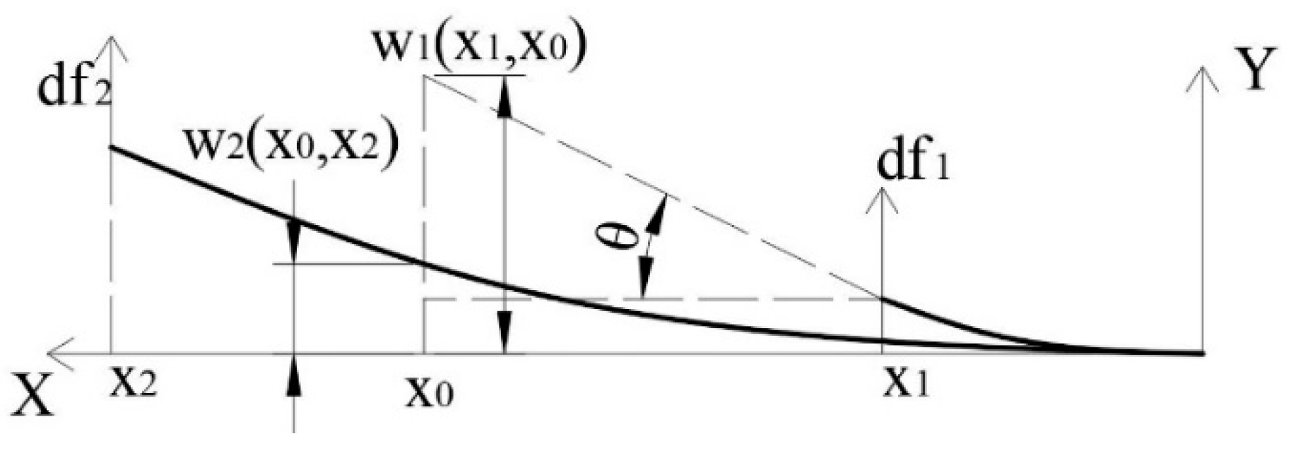
Figure A1.
Schematics of beam deflection. The total deflection is the sum of and . Both and are calculated by regarding the distributed load as infinite numbers of small point loads. The coordinate is not the same as the coordinate used in Figure 4.
Figure A1.
Schematics of beam deflection. The total deflection is the sum of and . Both and are calculated by regarding the distributed load as infinite numbers of small point loads. The coordinate is not the same as the coordinate used in Figure 4.
Now consider the deflection contributed by the distributed load at where . The contribution by a small point load at is expressed as:
where . The total deflection contributed by distributed load at to the point at can be derived as:
Thus, the total deflection can be derived as the sum of the Equations (A4) and (A6)
where is expressed in Equation (6).
The strain energy stored in the beam can be calculated by the work done by the distributed load
The energy release rate is expressed as
where
According to the well known relationship between the energy release rate and the stress intensity factor , , the stress intensity factor can be expressed as Equation (5).
References
- Germanovich, L.N.; Astakhov, D.K.; Mayerhofer, M.J.; Shlyapobersky, J.; Ring, L.M. Hydraulic fracture with multiple segments I. Observations and model formulation. Int. J. Rock Mech. Min. Sci. 1997, 34, 97.e1–97.e19. [Google Scholar] [CrossRef]
- Garagash, D.I.; Detournay, E.; Adachi, J.I. Multiscale tip asymptotics in hydraulic fracture with leak-off. J. Fluid Mech. 2011, 669, 260–297. [Google Scholar] [CrossRef]
- Sachau, T.; Bons, P.D.; Gomez-Rivas, E. Transport efficiency and dynamics of hydraulic fracture networks. Front. Phys. 2015, 3, 63. [Google Scholar] [CrossRef]
- Yew, C.H.; Weng, X. Mechanics of hydraulic fracturing. Gulf Prof. Publ. 2014, 23, 164–166. [Google Scholar]
- Cao, T.D.; Hussain, F.; Schrefler, B.A. Porous media fracturing dynamics: Stepwise crack advancement and fluid pressure oscillations. J. Mech. Phys. Solids 2018, 111, 113–133. [Google Scholar] [CrossRef]
- Abe, H.; Keer, L.M.; Mura, T. Growth rate of a penny-shaped crack in hydraulic fracturing of rocks, 2. J. Geophys. Res. 1976, 81, 6292–6298. [Google Scholar] [CrossRef]
- Garagash, D.; Detournay, E. The tip region of a fluid-driven fracture in an elastic medium. J. Appl. Mech. 2000, 67, 183–192. [Google Scholar] [CrossRef]
- Jeffrey, R.G. The combined effect of fluid lag and fracture toughness on hydraulic fracture propagation. In Low Permeability Reservoirs Symposium. Soc. Petroleum Eng. 1989. [Google Scholar] [CrossRef]
- Yew, C.H.; Liu, G.F. The fracture tip and KIc of a hydraulically induced fracture. Spe Prod. Eng. J. 1991, 171–177. [Google Scholar]
- Bunger, A.P.; Gordeliy, E.; Detournay, E. Comparison between laboratory experiments and coupled simulations of saucer-shaped hydraulic fractures in homogeneous brittle-elastic solids. J. Mech. Phys. Solids 2013, 61, 1636–1654. [Google Scholar] [CrossRef]
- Khoei, A.R.; Vahab, M.; Haghighat, E.; Moallemi, S. A mesh-independent finite element formulation for modeling crack growth in saturated porous media based on an enriched-FEM technique. Int. J. Fract. 2014, 188, 79–108. [Google Scholar] [CrossRef]
- Kostov, N.M.; Ning, J.; Gosavi, S.V.; Gupta, P.; Kulkarni, K.; Sanz, P.F. Dynamic hydraulic fracture modeling for wellbore integrity prediction in a porous medium. In Proceedings of the 2015 SIMULIA Community Conference, Berlin, Germany, 18–21 May 2015. [Google Scholar]
- Chang, H. Hydraulic Fracturing in Particulate Materials. Ph.D. Thesis, Georgia Institute of Technology, Atlanta, Georgia, 2004. [Google Scholar]
- Frash, L.P. Laboratory-Scale Study of Hydraulic Fracturing in Heterogeneous Media for Enhanced Geothermal Systems and General Well Stimulation. Ph.D. Thesis, Colorado School of Mines, Golden, CO, USA, 2014. [Google Scholar]
- Lhomme, T.P.; De Pater, C.J.; Helfferich, P.H. Experimental study of hydraulic fracture initiation in Colton sandstone. In Proceedings of the SPE/ISRM Rock Mechanics Conference, Irving, TX, USA, 20–23 October 2002. [Google Scholar]
- Lhomme, T.P.Y. Initiation of Hydraulic Fractures in Natural Sandstones. Ph.D. Thesis, Delft University of Technology, Delft, The Netherlands, 2005. [Google Scholar]
- Pizzocolo, F.; Huyghe, J.M.; Ito, K. Mode I crack propagation in hydrogels is step wise. Eng. Fract. Mech. 2013, 97, 72–79. [Google Scholar] [CrossRef]
- Tan, P.; Jin, Y.; Han, K.; Hou, B.; Chen, M.; Guo, X.; Gao, J. Analysis of hydraulic fracture initiation and vertical propagation behavior in laminated shale formation. Fuel 2017, 206, 482–493. [Google Scholar] [CrossRef]
- Wu, R. Some Fundamental Mechanisms of Hydraulic Fracturing. Ph.D. Thesis, Georgia Institute of Technology, Atlanta, Georgia, 2006. [Google Scholar]
- Wu, R.; Bunger, A.P.; Jeffrey, R.G.; Siebrits, E. A comparison of numerical and experimental results of hydraulic fracture growth into a zone of lower confining stress. In Proceedings of the 42nd US Rock Mechanics Symposium (USRMS), San Francisco, CA, USA, 29 June–2 July 2008. [Google Scholar]
- Zhang, G.Q.; Chen, M. Dynamic fracture propagation in hydraulic re-fracturing. J. Pet. Sci. Eng. 2010, 70, 266–272. [Google Scholar] [CrossRef]
- Zhou, J.; Chen, M.; Jin, Y.; Zhang, G.Q. Analysis of fracture propagation behavior and fracture geometry using a tri-axial fracturing system in naturally fractured reservoirs. Int. J. Rock Mech. Min. Sci. 2008, 45, 1143–1152. [Google Scholar] [CrossRef]
- Fisher, M.K.; Warpinski, N.R. Hydraulic-fracture-height growth: Real data. Spe Prod. Oper. 2012, 27, 8–19. [Google Scholar] [CrossRef]
- Bosanquet, C.H. LV. on the flow of liquids into capillary tubes. Lond. Edinb. Dublin Philos. Mag. J. Sci. 1923, 45, 525–531. [Google Scholar] [CrossRef]
- Xing, P.; Yoshioka, K.; Adachi, J.; El-Fayoumi, A.; Bunger, A.P. Laboratory measurement of tip and global behavior for zero-toughness hydraulic fractures with circular and blade-shaped (PKN) geometry. J. Mech. Phys. Solids 2017, 104, 172–186. [Google Scholar] [CrossRef]
- Bunger, A.P. Near-Surface Hydraulic Fracture. Ph.D. Thesis, University of Minnesota, Minneapolis, MN, USA, 2005. [Google Scholar]
- Bunger, A.P.; Detournay, E. Experimental validation of the tip asymptotics for a fluid-driven crack. J. Mech. Phys. Solids 2008, 56, 3101–3115. [Google Scholar] [CrossRef]
- Desroches, J.; Detournay, E.; Lenoach, B.; Papanastasiou, P.; Pearson, J.R.A.; Thiercelin, M.; Cheng, A. The crack tip region in hydraulic fracturing. Proc. R. Soc. Lond. A 1994, 447, 39–48. [Google Scholar] [CrossRef]
- Nordgren, R.P. Propagation of a vertical hydraulic fracture. Soc. Pet. Eng. J. 1972, 12, 306–314. [Google Scholar] [CrossRef]
- Perkins, T.K.; Kern, L.R. Widths of Hydraulic Fractures. J. Pet. Technol. 1961, 13, 937–949. [Google Scholar] [CrossRef]
- Kanninen, M.F. An augmented double cantilever beam model for studying crack propagation and arrest. Int. J. Fract. 1973, 9, 83–92. [Google Scholar]
- Fett, T.; Munz, D. Stress intensity factors and weight functions. Comput. Mech. 1997, 1, 112–115. [Google Scholar]
- Levenberg, K. A Method for the Solution of Certain Problems in Least-Squares. Q. Appl. Math. 1944, 2, 164–168. [Google Scholar] [CrossRef]
- Marquardt, D. An Algorithm for Least-squares Estimation of Nonlinear Parameters. Siam J. Appl. Math. 1963, 11, 431–441. [Google Scholar] [CrossRef]
- Yates, J.R.; Zanganeh, M.; Tai, Y.H. Quantifying crack tip displacement fields with DIC. Eng. Fract. Mech. 2010, 77, 2063–2076. [Google Scholar] [CrossRef]
- Schechter, R.S.; Wade, W.H.; Wingrave, J.A. Sorption isotherm hysteresis and turbidity phenomena in mesoporous media. J. Colloid Interface Sci. 1977, 59, 7–23. [Google Scholar] [CrossRef]
- Ridgway, C.J.; Gane, P.A.; Schoelkopf, J. Effect of capillary element aspect ratio on the dynamic imbibition within porous networks. J. Colloid Interface Sci. 2002, 252, 373–382. [Google Scholar] [CrossRef]
- Garagash, D.I. Propagation of a plane-strain hydraulic fracture with a fluid lag: Early-time solution. Int. J. Solids Struct. 2006, 43, 5811–5835. [Google Scholar] [CrossRef] [Green Version]
- Hunsweck, M.J.; Shen, Y.; Lew, A.J. A finite element approach to the simulation of hydraulic fractures with lag. Int. J. Numer. Anal. Methods Geomech. 2013, 37, 993–1015. [Google Scholar] [CrossRef]
- Vahab, M.; Khalili, N. Computational Algorithm for the Anticipation of the Fluid-Lag Zone in Hydraulic Fracturing Treatments. Int. J. Geomech. 2018, 18, 04018139. [Google Scholar] [CrossRef]
- Rubin, A.M. Propagation of magma-filled cracks. Annu. Rev. Earth Planet. Sci. 1995, 23, 287–336. [Google Scholar] [CrossRef]
- Xia, Y.; Jin, Y.; Chen, M.; Chen, K.P. An Enriched Approach for Modeling Multiscale Discrete-Fracture/Matrix Interaction for Unconventional-Reservoir Simulations. SPE J. 2018. [Google Scholar] [CrossRef]
- Zeng, C.; Deng, W. The Effect of Radial Cracking on the Integrity of Asperity Under Thermal Cooling Process. In Proceedings of the 52nd US Rock Mechanics/Geomechanics Symposium, Seattle, WA, USA, 17–20 June 2008. [Google Scholar]
- Dong, J.; Chen, M.; Jin, Y.; Hong, G.; Zaman, M.; Li, Y. Study on micro-scale properties of cohesive zone in shale. Int. J. Solids Struct. 2019, in press. [Google Scholar] [CrossRef]
- Li, Y.; Jia, D.; Rui, Z.; Peng, J.; Fu, C.; Zhang, J. Evaluation method of rock brittleness based on statistical constitutive relations for rock damage. J. Pet. Sci. Eng. 2017, 153, 123–132. [Google Scholar] [CrossRef]
- Li, Y.; Zuo, L.; Yu, W.; Chen, Y. A Fully Three Dimensional Semianalytical Model for Shale Gas Reservoirs with Hydraulic Fractures. Energies 2018, 11, 436. [Google Scholar] [CrossRef]
- Li, Y.; Rui, Z.; Zhao, W.; Bo, Y.; Fu, C.; Chen, G.; Patil, S. Study on the mechanism of rupture and propagation of T-type fractures in coal fracturing. J. Nat. Gas Sci. Eng. 2018, 52, 379–389. [Google Scholar] [CrossRef]
- Li, Y.W.; Zhang, J.; Liu, Y. Effects of loading direction on failure load test results for Brazilian tests on coal rock. Rock Mech. Rock Eng. 2016, 49, 2173–2180. [Google Scholar] [CrossRef]
- Geng, Z.; Bonnelye, A.; Chen, M.; Jin, Y.; Dick, P.; David, C.; Fang, X.; Schubnel, A. Time and Temperature Dependent Creep in Tournemire Shale. J. Geophys. Res. Solid Earth 2018, 123, 9658–9675. [Google Scholar] [CrossRef]
- Geng, Z.; Bonnelye, A.; Chen, M.; Jin, Y.; Dick, P.; David, C.; Fang, X.; Schubnel, A. Elastic anisotropy reversal during brittle creep in shale. Geophys. Res. Lett. 2017, 44, 21. [Google Scholar] [CrossRef]
- Jin, Y.; Chen, K.P.; Chen, M. An asymptotic solution for fluid production from an elliptical hydraulic fracture at early-times. Mech. Res. Commun. 2015, 63, 48–53. [Google Scholar] [CrossRef]
- Siddhamshetty, P.; Kwon, J.S.; Liu, S.; Valkó, P.P. Feedback control of proppant bank heights during hydraulic fracturing for enhanced productivity in shale formations. Aiche J. 2018, 64, 1638–1650. [Google Scholar] [CrossRef]
- Siddhamshetty, P.; Yang, S.; Kwon, J.S. Modeling of hydraulic fracturing and designing of online pumping schedules to achieve uniform proppant concentration in conventional oil reservoirs. Comput. Chem. Eng. 2018, 114, 306–317. [Google Scholar] [CrossRef]
Figure 1.
The experimental setup and specimen configuration. (a) Laboratory-scale hydraulic fracturing device. The high-speed camera direction is parallel to the specimen surface and the optical microscope direction is perpendicular to the specimen surface. Both the specimen and frame are transparent; (b) Configuration of the hydraulic fracture in double-cantilever-beam (HF-DCB) specimen. The to-be-fractured area is pasted with 0.05 mm thin copper foil to avoid side flow; (c) HF-DCB with intrinsically sharp crack tip induced by Chevron notch.
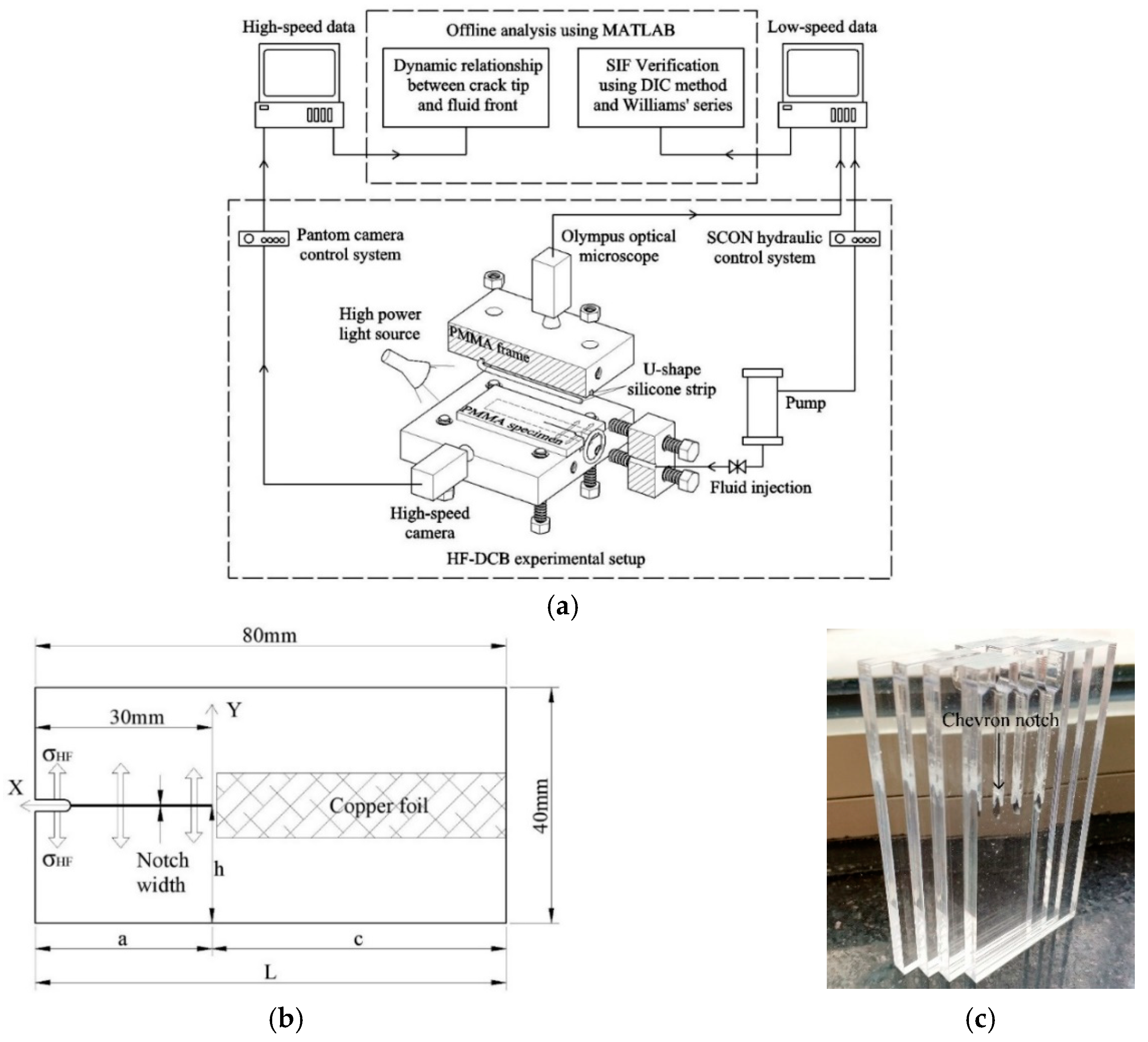
Figure 2.
Comparison between stress intensity factor (SIF) between the analytic solution (Equation (9)) using beam theory and the Fett’s result (Equation (12)) using boundary collocation method and the weight functions. for . The two results show good agreement with each other in a wide range. The variables on the horizontal and the vertical coordinates are dimensionless numbers.
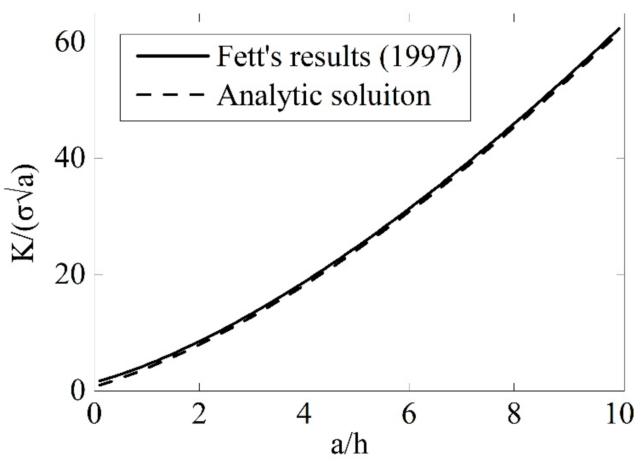
Figure 3.
Comparison between theoretical SIF results and experimental SIF results. The theoretical SIFs are derived using Equation (9). The experimental SIFs are derived using a combined method of Digital Image Correlation (DIC) full-field displacement extraction and the fitting of DIC full-field displacement extraction and the fitting of Williams’ series. Williams’ series. The specimens are loaded to the SIF that is slightly lower than the fracture toughness.

Figure 4.
Illustration of dynamic fluid analyses in the crack. The coordinate origin is where the crack starts to propagate. The crack profile is assumed to stay the same while propagating. is the position of the fluid front. is the point for the integral analyses in the fluid. D is the crack opening width. The upper part of the figure is the illustration of the analyses of the crack flank resistance.
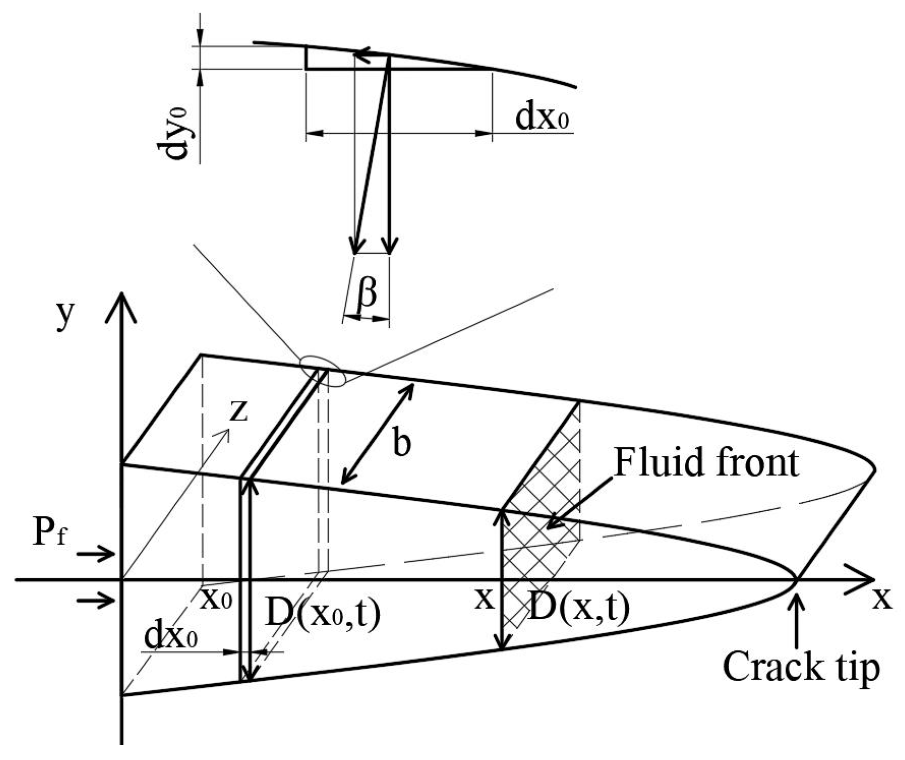
Figure 5.
Comparison between quasi-static beam deflection and the approximation of linear crack profile. The quasi-static beam deflection is derived using beam theory. The linear crack profile provides a good approximation of the crack profile in the considered area.
Figure 5.
Comparison between quasi-static beam deflection and the approximation of linear crack profile. The quasi-static beam deflection is derived using beam theory. The linear crack profile provides a good approximation of the crack profile in the considered area.

Figure 6.
(a,b) are the comparison between experimental results and theoretical results of fluid front for sample #12 (fracturing pressure: 2.74 MPa) and sample #14 (fracturing pressure: 4.06 MPa) respectively. The fluid front positions are the numerical results by solving Equation (22) with and without the term of the crack flank resistance. The calculations with the crack flank resistance term provide better results of the fluid front position; (c,d) are corresponding energy as a function of time. The energy terms are calculated using the equations from Equation (23) to Equation (26). The kinetic energy of the fluid occupies around half of the total energy. The work done by the fluid on the crack flank is a non-negligible part of the total energy. The input energy and the consumed energy conform well to each other.

Figure 7.
(a,b) are comparison between experimental results and theoretical results of fluid front for sample #15 (fracturing pressure: 2.64 MPa) and sample #16 (fracturing pressure: 2.53 MPa) respectively. The fluid front positions are the numerical results by solving Equation (22) with and without the term of the crack flank resistance. The calculations with the crack flank resistance term provide much more realistic results of the fluid front position; (c,d) are corresponding energy as a function of time. The kinetic energy of the fluid occupies over half of the total energy. stops increasing after the arrest of the crack as expected. The input energy and the consumed energy conform well to each other.
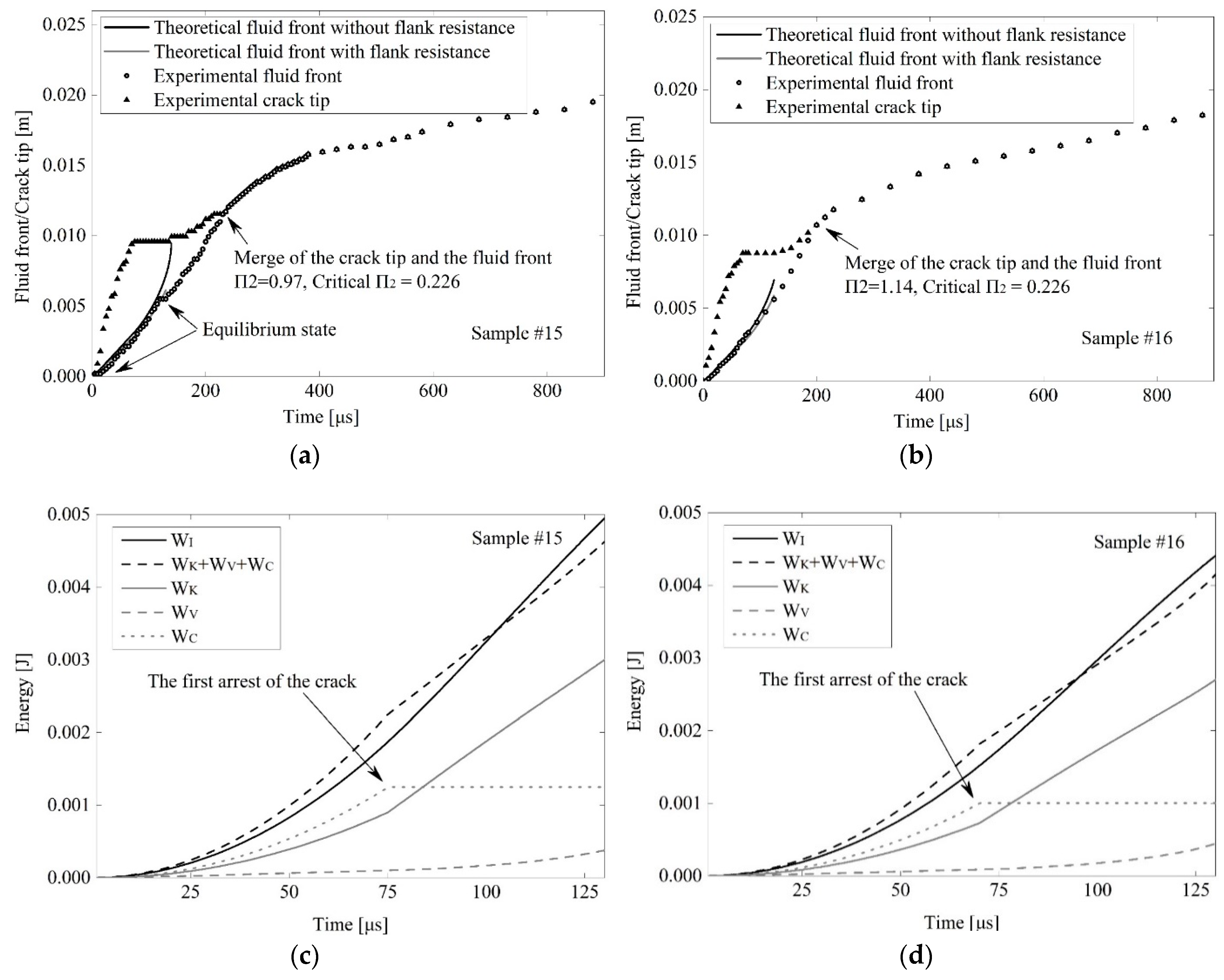
Figure 8.
Dynamic images of the relationship between crack tip and fluid front of sample #12. The direction of the high-speed camera is shown in Figure 1a. The crack tip and the fluid front separate at the beginning of the propagation, and the fluid front catches up with the crack tip when it slows down. The phenomenon of fluid ejection presents when the fluid front approaches the crack tip, and meanwhile the fluid velocity is theoretically high but actually low in the real case.

Figure 9.
and as a function of . The solid line is the criterion of the existence of the equilibrium state. It is valid regardless of on the right of the dot line (), and is valid only when on the left of the dot line. The maximum equilibrium velocity indicates the equilibrium velocity when .
Figure 9.
and as a function of . The solid line is the criterion of the existence of the equilibrium state. It is valid regardless of on the right of the dot line (), and is valid only when on the left of the dot line. The maximum equilibrium velocity indicates the equilibrium velocity when .

Figure 10.
Numerical results of dimensionless fluid velocity as a function of time under different and viscosity . These numerical results are obtained using liner profile, , , and . There is no equilibrium state when . The initial “slow down” at the time of is an artificial result of the initial value of the numerical calculation. The numerical results conform well to the theoretical prediction of .

Figure 11.
(a) Comparison between numerical and theoretical equilibrium fluid velocity as a function of for different crack profiles. The numerical results are derived by solving Equation (22). The theoretical results are from Equation (33). Some typical profiles are investigated; (b) Comparison between experimental and theoretical equilibrium fluid velocity as a function of for . The experimental results of equilibrium fluid velocity are extracted from the latter half of the equilibrium state as shown in Figure 7a.
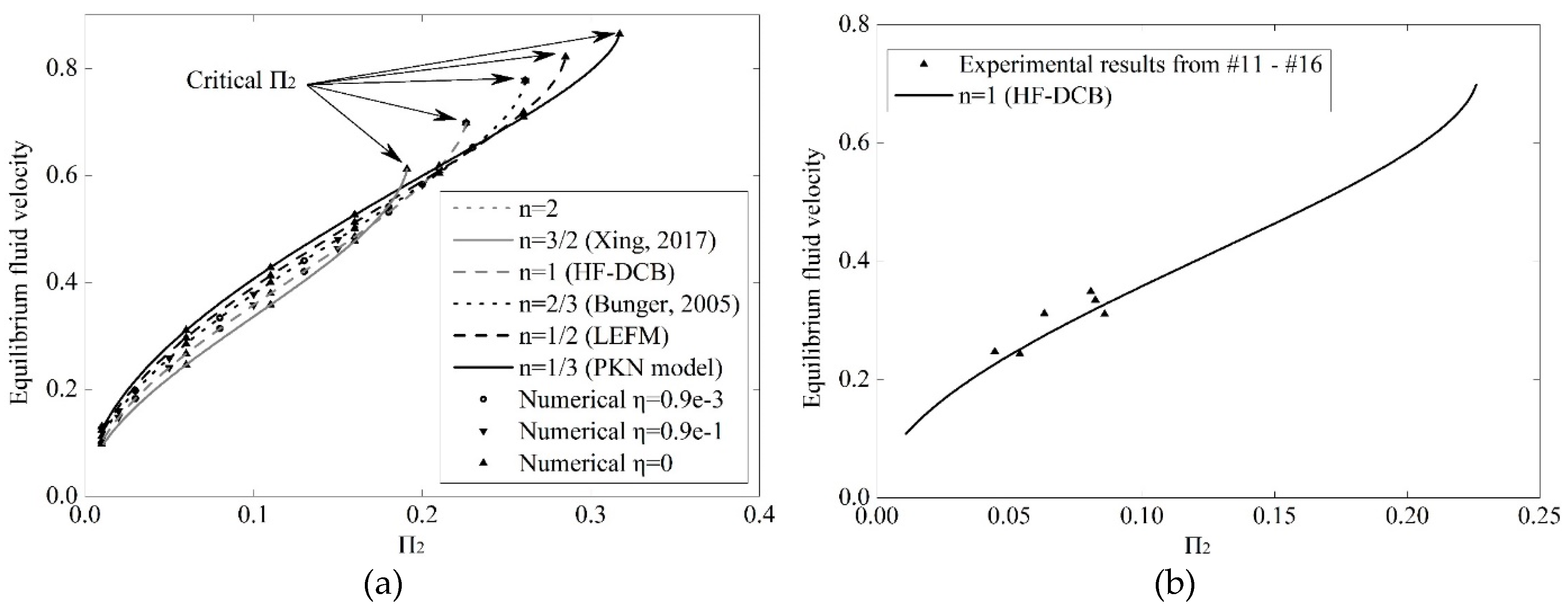
Figure 12.
Verification of and compared with experimental results. The massive data on the left are extracted from varies experiments in which cracks propagate in a stepwise manner and never separate with fluid fronts. Two of the data points close to the curve of are shown in Figure 7a,b. The sporadic data on the right are the initiation parts of the cracks in the experiments, which are prone to the separation due to the high speed of crack tip. Both and provide good predictions of the experimental results.


Table 1.
Sample data.
| NO. | Crack Notch Width (mm) | Initial Crack Length (mm) | Fracturing Pressure (MPa) | Initiation Toughness * |
|---|---|---|---|---|
| #5 | Intrinsically sharp crack | 35 | 1.95 | 2.52 |
| #6 | Intrinsically sharp crack | 35 | 1.72 | 2.22 |
| #7 | Intrinsically sharp crack | 37 | 1.52 | 2.15 |
| #11 | 0.5 | 30 | 3.56 | 3.62 |
| #12 | 0.5 | 30 | 2.74 | 2.78 |
| #13 | 0.5 | 30 | 2.26 | 2.30 |
| #14 | 2.0 | 30 | 4.06 | 4.13 |
| #15 | 2.0 | 30 | 2.64 | 2.68 |
| #16 | 2.0 | 30 | 2.53 | 2.57 |
* According to our preliminary study, the initiation toughness is related to both the crack notch width and the pressure-hold time before initiation which results in craze and blunting in the near-tip region.
© 2019 by the authors. Licensee MDPI, Basel, Switzerland. This article is an open access article distributed under the terms and conditions of the Creative Commons Attribution (CC BY) license (http://creativecommons.org/licenses/by/4.0/).
Share and Cite
MDPI and ACS Style
Dong, J.; Chen, M.; Li, Y.; Wang, S.; Zeng, C.; Zaman, M. Experimental and Theoretical Study on Dynamic Hydraulic Fracture. Energies 2019, 12, 397. https://doi.org/10.3390/en12030397
AMA Style
Dong J, Chen M, Li Y, Wang S, Zeng C, Zaman M. Experimental and Theoretical Study on Dynamic Hydraulic Fracture. Energies. 2019; 12(3):397. https://doi.org/10.3390/en12030397
Chicago/Turabian StyleDong, Jingnan, Mian Chen, Yuwei Li, Shiyong Wang, Chao Zeng, and Musharraf Zaman. 2019. "Experimental and Theoretical Study on Dynamic Hydraulic Fracture" Energies 12, no. 3: 397. https://doi.org/10.3390/en12030397
Note that from the first issue of 2016, this journal uses article numbers instead of page numbers. See further details here.