Forecasting the Energy Embodied in Construction Services Based on a Combination of Static and Dynamic Hybrid Input-Output Models

Abstract

The energy embodied in construction services (EECS) to increase industrial production capacity, contributes to total primary energy consumption (TPEC) in developing countries like China. Forecasting EECS is important for creating energy policies, but has not received enough attention. There are some defects in the main two methods of EECS forecasting: the static hybrid input-output (HI/O) model and the dynamic HI/O model. The former cannot identify the quantity of construction services, whereas the latter is unstable for EECS forecasting. To tackle these problems, we propose a new model, which is a combination of the static and dynamic hybrid input-output model (CSDHI/O model), for EECS forecasting. Taking China as a case study, we forecast the EECS and TPEC of China until 2020 and analyze the sensitivities of four influencing factors. The results show that the EECS of China will reach 1.79 billion tons of coal equivalent in 2020. The improvement of fabrication level is identified as the most important factor for conserving both TPEC and EECS. A sudden drop in gross domestic product (GDP) growth rate and decreasing the investment in the service industry can also restrict EECS growth.

1. Introduction

The notion of reducing greenhouse gas emissions to mitigate climate change has been accepted by many economies and scholars. Conserving fossil energy consumption is an important way to reduce such emissions. In addition to increasing the proportion of renewable energy, reducing the demand for energy services is another major measure to conserve fossil energy. Forecasting the demand for energy services is a basic task in reducing the demand for energy services, which has received much attention by many countries and research institutions.

The demand for energy services can be divided into two categories: construction services and operation services [1]. During economic development, some energy is consumed by construction services for increasing the production capacity of various sectors. Correspondingly, the energy consumed by operation services is used to maintain the current production capacity. For rapidly developing economies like China, the energy embodied in construction services (EECS) can be quite large. In 2007, the EECS, as estimated by the energy embodied in the fixed assets investments (FAI), consumed one-third of the total energy in China [2]. A recent study [3] also showed that EECS was the top final consumer of embodied energy in Beijing in 2010. Therefore, for economies experiencing rapid development, it is important to forecast EECS and analyze its influencing factors in order to control energy consumption and related emissions.

However, in the energy consumption forecasting literature [4,5,6,7,8,9,10,11,12,13,14,15,16,17,18,19,20,21,22,23,24,25,26,27,28,29,30,31], few studies separate EECS from total primary energy consumption (TPEC). Most previous studies on EECS [2,3,32] are historical analyses and estimate EECS using the energy embodied in FAI. In both forecasting studies and historical analyses, the hybrid input-output model (HI/O model) is widely adopted [2,4,5,6,7,8,9,32,33,34,35,36,37,38,39,40,41,42,43,44,45,46,47] because it is based on the inherent law of energy-economics and clearly explains the internal mechanism for economic growth by the change in sectoral product demand, to the change in energy consumption. More importantly, the HI/O model is the main method used to extract EECS from TPEC.

The difficulty in forecasting EECS is mainly due to the limitation of existing HI/O models, which can be classified as static models and dynamic models. Although static HI/O models are more stable in TPEC forecasting, the quantity of FAI is an exogenous variable and so cannot respond to changes in sectoral product demand. The dynamic HI/O models can decompose EECS by establishing the quantitative relationship between FAI and the output increment of various sectors, but the forecast is unstable because of the singularity of the natural capital coefficient matrix and the inability to decompose the direct input coefficient matrix. Thus, a combination of static and dynamic HI/O models can create a better method that is both stable and functional for EECS forecasting, an idea which deserves further study.

The aim of this paper was to develop a method of EECS forecasting, called the CSDHI/O model, based on the combination of static and dynamic hybrid input-output models. The CSDHI/O model forecasts TPEC using static methods based on gross domestic product (GDP) prediction, and estimates the EECS along with the economic prediction using dynamic methods. Thus, by combining the advantages of static HI/O methods and dynamic HI/O methods, we can better forecast and analyze EECS. The establishment of the CSDHI/O model includes five steps. First, we build HI/O tables based on historical data to prepare the basic energy and economic data for our forecast. Second, we predict the final demand of each sector. Third, the output and TPEC of the economy is forecast by applying static methods in the HI/O model. Fourth, we estimate EECS, which is essential for meeting the product demands of various sectors using dynamic methods. Finally, we conduct sensitivity analysis of various influencing factors of EECS forecasting and TPEC forecasting. To demonstrate the CSDHI/O model, the forecast of TPEC and EECS of China until 2020 is used as a case study, because China is a rapidly developing economy with the largest energy consumption and carbon emissions in the world.

The main contributions of this paper include: (1) we develop a CSDHI/O model to forecast the EECS of an economy based on the GDP prediction, which reveals the dynamic relationship between economic development and EECS. This is an early attempt of methodology development to forecast the EECS in the process of economic development. The CSDHI/O model originally combines the forecasting stability of the static HI/O model and the dynamic characteristics of FAI, growing with product demands in the dynamic HI/O model. (2) In applying the CSDHI/O model, we forecast the EECS of China until 2020 and analyze its influencing factors. Through sensitivity analysis of the CSDHI/O model, we deepen our understanding of the influencing factors of EECS forecasting, and find effective measures to conserve EECS and TPEC. Based on the results, we draw policy implications for the conservation of EECS and TPEC in China.

The paper is organized as follows: related literature is reviewed in Section 2. Section 3 introduces the methodology and data preparation. Section 4 presents the results and sensitivity analysis. Section 5 summarizes the conclusions and provides policy implications.

2. Literature Review

Energy consumption forecasting is a basic task in creating energy policies. Many organizations, such as BP [10,11], the International Energy Agency [12], the Chinese Academy of Engineering [13], and Chinese Energy Research Institute [14] have regularly published energy consumption forecasts for various countries and regions around the world. Energy consumption forecasting has always been a popular issue in academic research. Many scholars have studied various methods of energy consumption forecasting, which can be classified into three categories: (1) artificial intelligence forecasting models, including genetic algorithms [15,16], artificial neural networks [17,18,19,20], and swarm intelligence optimization [15,16,21]; (2) grey forecasting models [22,23,24,25]; and (3) econometric models, such as the HI/O model [2,4,5,6,7,8,9], the integrated MARKAL-EFOM system model [26], the macroeconomic Bayesian vector autoregression model [27], the autoregressive integrated moving average model [28,29,30], and other econometric models [31].

Most of these studies focused on TPEC forecasting and analyzed the influencing factors of TPEC, including economic development (GDP growth rate, per capita GDP), economic structure (consumption structure change, industrial structure change), and technological change (substitution, fabrication level). However, little attention has been paid to forecasting EECS caused by economic development and the influencing factors.

EECS indicates the energy embodied in construction services-related fixed assets investment (CSFAI), which accounts for the majority of the total FAI [48]. Embodied energy analysis of various final demand products in an economy, including FAI or CSFAI, is mostly based on the HIO model, which has been transformed from the traditional input-output model [49]. Most studies on embodied energy analysis estimated primary energy embodied in products and services, or in the trade between economies, such as the energy embodied in the global production system [33], the energy requirements of Sydney households [34], the primary energy and greenhouse gas embodied in Australian final consumption [35], the energy requirements of Brazil households [36], energy-related carbon emission of Irish construction sector [32], the embodied energy of industrial sectors of China [37], the energy embodied in international trade of China [38,39]. A few researchers estimated the energy embodied in FAI, which was taken as EECS, based on historical data analysis. Fu et al. [2] estimated the EECS of China and concluded that EECS accounted for one-third of the TPEC of China in 2007. Li et al. [3] estimated the EECS of Beijing and confirmed that EECS was the largest type of embodied energy of Beijing in 2010. Acquaye et al. [32] estimated the energy-related carbon emission of Irish construction sector, which is highly correlated with TPEC. The results showed that the energy-related carbon emission of construction sector accounted for 11% of the total domestically arising CO₂ emissions of Ireland in 2005. In EECS-related studies, the HI/O model was the most popular method applied. However, few studies involved EECS forecasting. The lack of research on EECS forecasting is speculated to be partly due to insufficient attention paid by scholars to EECS in rapidly developing economies, and partly to the limitation of existing HI/O models.

The HI/O model can be divided into two categories, which are static HI/O models and dynamic HI/O models, but each category has limitations for EECS forecasting. The static HI/O models can forecast the TPEC of the economy based on GDP prediction, but does not accurately simulate the dynamic changes in FAI. For example, Zheng et al. [8] forecasted China’s TPEC and carbon emissions embodied in the final demand products of various sectors. Zhang et al. [40] proposed a static hybrid input-output model of nine pieces to forecast the energy demand of Jiangsu Province. Hamilton et al. [41] developed a multi-regional input-output model for Africa to estimate the primary energy supply and energy-related carbon emissions along with the economic growth, and forecasted the primary energy supply and he energy-related carbon emissions of sub-Saharan Africa in 2030. Dejuán et al. [42] also built an input-output model, which can reflect the impact of fuel prices on energy demand in various sectors, to forecast the energy demand of Spain. However, due to the limitations of the static HI/O model, the FAI volume is an exogenous variable, which results in a mismatch between the quantity of FAI forecasted by the static HI/O model and the economic development. Thus, although the forecasting was stable, EECS cannot be forecasted by a static HI/O model.

Although the dynamic HI/O model has inherent advantages in estimating EECS, there are also some drawbacks in forecasting EECS with this model. For simulating the dynamic growth of FAI with the output increase of various sectors, the dynamic input-output model was developed by Leontief [43]. Compared to static input-output model, the dynamic input-output model contains a “capital coefficient”, which is defined as the ratio of FAI invested by one sector to the increase of its total output. With this coefficient, the FAI has changed into an endogenous variable of the model, and is considered to be the construction services caused by the change of the total output of each sector. The dynamic input-output model was introduced into the energy field in 1978 by Rhoten [44], who developed the dynamic energy-economy HI/O model. Penner [45] developed a partially dynamic input-output model of the United States economy, and examined the net energy costs of constructing and operating the energy-supply system. Recently, the dynamic HI/O model has been applied to forecast TPEC and energy-related carbon emissions under various optimization objectives [4,5,6,7], or be improved to analyze and estimate renewable energy [46] and bioenergy [47] with economic development. However, few studies have forecasted EECS or distinguished EECS from TPEC forecast. There are two main issues in EECS forecasting with the dynamic HI/O model: (1) The forecasts are based on the prediction of various sectors’ final demand, except FAI, and more specifically, excluding for CSFAI. However, most studies on energy consumption forecasting did not distinguish between FAI and CSFAI. Furthermore, it is difficult to separately predict the final demand without the CSFAI of each sector. (2) Forecasting with the dynamic HI/O model is very sensitive to the capital coefficient matrix and the direct input coefficient matrix. However, the capital coefficient matrix of an HI/O model is always a singular matrix with huge differences between the elements of various sectors. This characteristic of the capital coefficient matrix and the inability of the direct input coefficient matrix to be decomposed always leads to instability in solving the dynamic HI/O model [50,51]. This restricts the application of dynamic HI/O models to energy consumption forecasting. Therefore, dynamic HI/O models can be used for TPEC and EECS estimation and forecasting, but the forecast function is not stable.

Both the static HI/O model and the dynamic HI/O model have been applied to forecast TPEC, but they have some issues when EECS forecasting. Therefore, an EECS forecasting method should be developed by combining the two categories of HI/O models, which may overcome their respective defects.

3. Methodology and Data Preparation

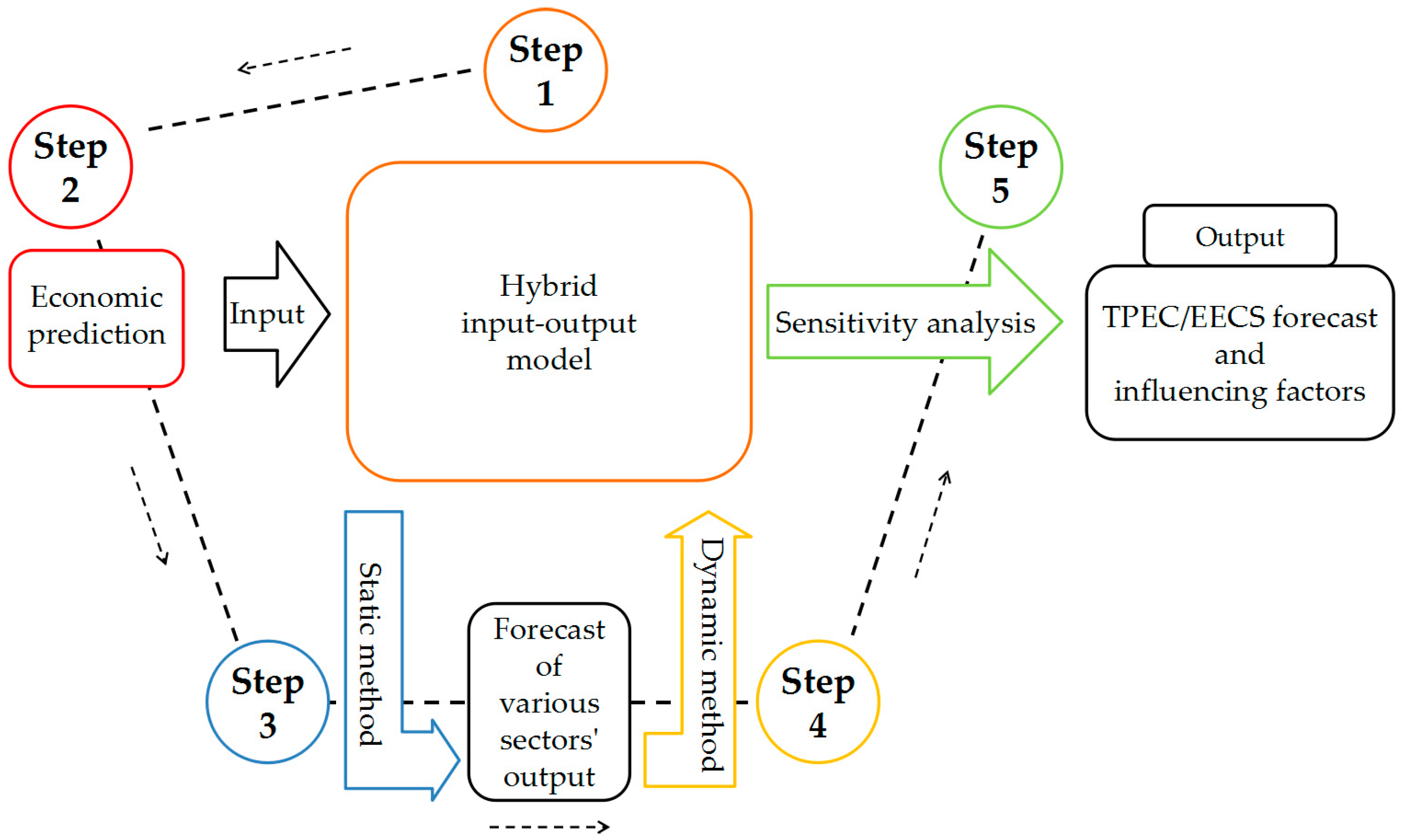
In this section, we first introduce the establishment of the CSHI/O model, and then describe the preparation of data for the case study.

3.1. CSDHI/O Model

We attempted to combine the advantages of the static HI/O model and the dynamic HI/O model to build a new model, called the CSDHI/O model, to forecast EECS based on GDP prediction and analyze the influencing factors using sensitivity analysis. Specifically, we applied the static method in the HI/O model to forecast TPEC caused by the final demand increase of various sectors. We used the dynamic method in the HI/O model to estimate the EECS necessary for an economy to develop as predicted. Developing the CSDHI/O model involved five steps, as shown in Figure 1:

• The first step (Step 1, the orange box in the middle of Figure 1) was to establish the HI/O tables and prepare data for forecasting, which can be considered establishing an HI/O model. Several coefficient matrices needed for forecasting were estimated based on historical data.
• The second step (Step 2, the red box in Figure 1) was to predict the economic development. Specifically, we predicted the final demand of each sector, which was the basis for the EECS forecasting. The economic prediction was the input of the CSDHI/O model.
• The third step (Step 3, the blue part in Figure 1) was to forecast the output of various sectors according to the economic prediction by applying the static method in the HI/O model.
• The fourth step (Step 4, the yellow part in Figure 1) involved estimating the EECS caused by the output increase of various sectors by applying the dynamic method in the HI/O model. The output increase of various sectors forecasted by Step 3 was the input of Step 4.
• The last step (Step 5, the green part in Figure 1) involved conducting sensitivity analysis of the various influencing factors of EECS and TPEC to identify the impact of each factor on EECS and TPEC growth. The GDP growth rate, proportion of final demand of each sector, fabrication level, and the positive capital coefficient are recommended for the sensitivity analysis.

3.1.1. Establishment of HI/O Tables

The energy-economic HI/O model is operated based on energy-economic HI/O tables, which were created by replacing the economic value of the energy sector in the conventional economic input-output table with the physical quantity of various types of energy. The typical energy-economic HI/O table of an economy with n intermediate sectors, of which m is the energy sector, is shown in

Table 1. A typical energy-economic hybrid input-output table year t, where * represents the physical quantity of energy.

		Intermediate Sector				Final Demand				Output
		1	2	…	n	Final Consumption	Net Export	Fixed Assets Investment	Other Final Demand
Intermediate Sectors	1	${z^{\ast }}_{11}^t$	${z^{\ast }}_{12}^t$	…	${z^{\ast }}_{1n}^t$	${f^{\ast }}_{\mathrm{FC},1}^t$	${f^{\ast }}_{\mathrm{NE},1}^t$	${f^{\ast }}_{\mathrm{FAI},1}^t$	${f^{\ast }}_{\mathrm{OFD},1}^t$	${x^{\ast }}_1^t$
	2	${z^{\ast }}_{21}^t$	${z^{\ast }}_{22}^t$	…	${z^{\ast }}_{2n}^t$	${f^{\ast }}_{\mathrm{FC},2}^t$	${f^{\ast }}_{\mathrm{NE},2}^t$	${f^{\ast }}_{\mathrm{FAI},2}^t$	${f^{\ast }}_{\mathrm{OFD},2}^t$	${x^{\ast }}_2^t$
	⋮	⋮	⋮	⋮	⋮	⋮	⋮	⋮	⋮	⋮
	m	${z^{\ast }}_{m1}^t$	${z^{\ast }}_{m2}^t$	…	${z^{\ast }}_{mn}^t$	${f^{\ast }}_{\mathrm{FC},m}^t$	${f^{\ast }}_{\mathrm{NE},m}^t$	${f^{\ast }}_{\mathrm{FAI},m}^t$	${f^{\ast }}_{\mathrm{OFD},m}^t$	${x^{\ast }}_m^t$
	m + 1	$z_{(m+1)1}^t$	$z_{(m+1)2}^t$	…	$z_{(m+1)n}^t$	$f_{\mathrm{FC},m+1}^t$	$f_{\mathrm{NE},m+1}^t$	$f_{\mathrm{FAI},m+1}^t$	$f_{\mathrm{OFD},m+1}^t$	$x_{m+1}^t$
	⋮	⋮	⋮	⋮	⋮	⋮	⋮	⋮	⋮	⋮
	n	$z_{n1}^t$	$z_{n2}^t$	…	$z_{nn}^t$	$f_{\mathrm{FC},n}^t$	$f_{\mathrm{NE},n}^t$	$f_{\mathrm{FAI},n}^t$	$f_{\mathrm{OFD},n}^t$	$x_n^t$

Note: z represents the intermediate input; f stands for the final demand; x is various sectors’ output; and subscripts FC, NE, and OFD means final consumption, net export, and other final demand, respectively. The first number subscript means the row of the table and the second subscript means the column of the table. The specific establishing process of the hybrid tables was explained by Miller et al. [52].

.

There are some key coefficient matrices that had to be estimated. The direct input coefficient $a_{ij}^t$ can be defined with Equation (1). The direct input coefficient matrix, which is A matrix, is composed of direct input coefficients:

$$a_{ij}^t=\frac{z_{ij}^t}{x_j^t}$$

(1)

The proportion of fixed assets invested by sector j in sectors i is defined as pfai_ij. The fixed assets invested by sector j in sectors i in t year, $FA{I}_{ij}^t$, can be calculated by Equation (2):

$$FA{I}_{ij}^t=pfa{i}_{ij}^t·f_{FAI,i}^t$$

(2)

where $f_{FAI,i}^t$ is the total fixed assets invested in sector i in t year.

The proportion of CSFAI to FAI is assumed to be pcsfai^t, which is important for distinguishing between CSFAI and FAI. As mentioned before, the FAI invested by each sector can be divided into CSFAI and operation services-related FAI. The operation services-related FAI can be simply estimated by multiplying the net fixed assets and depreciation rate of the fixed assets in the sector. The net fixed assets and the total FAI invested by each sector can be obtained from the statistical data. Thus, the proportion of operation services-related FAI to the total FAI in each sector can be estimated. Considering this parameter plus pcsfai^t equals 100%, the pcsfai^t of each sector can be estimated. Usually, it is assumed that the depreciation rate of the fixed assets in the sector remains the same during the forecasting period. Therefore, the quantity of CSFAI can be estimated using Equation (3):

$$CSFA{I}_{ij}^t=pcsfa{i}_{ij}^t·FA{I}_{ij}^t$$

(3)

where $CSFA{I}_{ij}^t$ is the CSFAI of sector i invested by sector j of t year.

Based on the definition of $CSFA{I}_{ij}^t$, a positive capital coefficient, $C_{ij}^t$, derived from the traditional capital coefficient can be defined by Equation (4):

$$c_{ij}^t=CSFA{I}_{ij}^t/{\displaystyle \sum \Delta x_j^{t+}},\Delta x_j^{t+}\ge 0$$

(4)

where $\Delta x_j^{t+}$ is the positive difference between the output of sector j in t + 1 year and the output of sector j in t year. The specific definition and calculation of the positive capital coefficient are provided in Appendix A.

3.1.2. Prediction of Economic Development

The aim of Step 2 was to forecast the final demand of each sector according to the actual development state of the economy. The prediction of economic development was realized in two steps:

• Estimate the final demand of the primary industry, the secondary industry and the tertiary industry in the future, respectively. In input-output models, the GDP of the economy equals the sum of the final demand of various sectors. Therefore, we can calculate the total GDP according to the historical GDP data and the future GDP growth rate predicted by other institutions, and regard it as the total amount of final demand. It is assumed that the proportion of the final demand of the primary industry to the total final demand logarithmic changes with time, and the proportion of the final demand of the tertiary industry to the total final demand changes linearly with time. Through historical data, the least square method is used to fit the change formula of these two proportions. The proportion of the final demand of the secondary industry can be calculated by subtracting the sum of the proportion of the primary industry and the proportion of the tertiary industry from 100%. The final demand of each industry can be estimated as:

  $$f_{type}^t=f^t·pi{n}_{type}^t,type\in \left(primary,\sec ondary,tertiary\right)$$

  (5)

  where $f_{type}^t$ is the final demand of each industry in t year; f^t = ($f_1^t$, $f_2^t$, …, $f_n^t$)^T is n sectors’ final demands in t year; $pi{n}_{type}^t$ stands for the proportion of the final demand of each industry in t year.
• Predict the proportion of the final demand of each sector to the final demand of its industry. The final demand of sector i can be estimated as:

  $$f_i^t=f_{type}^t·ps{e}_{type,i}^t,type\in \left(primary,\sec ondary,tertiary\right)$$

  (6)

  where $f_i^t$ is the final demand of sector i in t year; $ps{e}_{type,i}^t$ stands for the proportion of the final demand of sector i to its industry in t year.

3.1.3. Forecast the Energy Consumption by the Static Method

In input-output models, the output of various sectors can be estimated using Equation (7):

$$x^t={(I-A^t)}^{-1}·f^t$$

(7)

where x^t = ($x_1^t$, $x_2^t$, …, $x_n^t$)^T is n sectors’ output in t year; I represents an identify matrix; A^t = (a_ij)^t is the direct input coefficient matrix in t year; and (I − A^t) should be a non-singular matrix.

The output of energy sectors in x^t is the embodied energy of the final demand. The embodied energy of all the final demand plus the net import is considered the TPEC of the economy. To forecast the energy consumption using Equation (7), it is necessary to forecast the direct input coefficient matrix in t year, A^t. In input-output models, the direct input coefficient matrix reflects the production structure of the economy. To forecast the A^t, the RAS procedure, improved by Toh [53], is adopted. The RAS procedure is commonly used to adjust the direct input coefficient matrix of the future based on the direct input coefficient matrix of the base year [7]. In the RAS procedure, the direct input coefficient matrix in t year is estimated as:

$$A^t=R·A^{t-1}·S$$

(8)

where R and S are two diagonal matrices. In the RAS procedure, the R matrix reflects the substitution of products in the intermediate production, whereas the S matrix reflects the fabrication level of various sectors. R and S are usually estimated by analyzing the change in matrix A in the history of the economy and predicting the production structure of various sectors.

3.1.4. Estimate the EECS Using the Dynamic Method

The EECS is the energy embodied in CSFAI, which is the output of energy sectors embodied in CSFAI. The output can be estimated using Equation (7). Therefore, it is crucial to identify the quantity of CSFAI when estimating EECS. The quantity of CSFAI can be estimated as:

$$CSFA{I}_{ij}^t=c_{ij}^t·\Delta x_j^{t+}$$

(9)

To differentiate the EECS result from the final demand change of various sectors and that result from technological change, the structural decomposition analysis is adopted in this step. The specific estimation of EECS is outlined in Appendix B. Considering the investment of each sector may change in the future, a correction coefficient, cc^t, for C^t matrix is introduced in this paper. The positive capital coefficient matrix C in t year can be estimated as:

$$C^t=c{c}^t·C^0$$

(10)

Besides the basic assumptions in the input-output model, there are three special assumptions in this CSDHI/O model: (1) FAI finishes within the same year it was invested, (2) FAI is used for production in years after investment finished, and (3) the capacity utilization rate of each sector remains the same in the forecast.

3.1.5. Sensitivity Analysis

The sensitivity analysis of various influencing factors of EECS and TPEC forecasting, such as the GDP growth rate, proportion of final demand of each sector, fabrication level in the RAS procedure, and the positive capital coefficient, was conducted. In sensitivity analysis, each influencing factor is assumed to change within its own ±20% range.

We set various scenarios by choosing the most effective influencing factor for reducing EECS and TPEC in each sensitivity analysis. Comparing the EECS and TPEC in each scenario can identify the relative impact of each factor on the conservation of EECS and TPEC.

3.2. Data Preparation

China is the largest energy consumer and carbon emitter in the world. Energy conservation is always an issue in China. According to the work of Fu et al. [2], the energy embodied in FAI accounts for a large part of China’s TPEC. Therefore, choosing China as a case study demonstrates the model well. In this paper, the economic and energy data for China from 2007 to 2012 were adopted as basic data to forecast the energy consumption and EECS from 2013 to 2020. The forecast result was compared with the statistical data published by National Bureau of Statistics (NBS) of China and forecast results of two institutes to verify the accuracy of the CSDHI/O model.

To establish the hybrid input-output table, the input-output tables for China of 2007 [54], 2010 [55], and 2012 [56], published by NBS, were adopted. The sectors of the original input-output tables were merged into 21 sectors, as shown in

Table 2. Sector setting.

Code	Sector (Abbreviation)	Sector (Full Name)
01	Coal	Mining and Washing of Coal
02	Petroleum and Natural Gas	Extraction of Petroleum and Natural Gas
03	Petroleum Processing	Processing of Petroleum, Coking, and Processing of Nuclear Fuel
04	Electric Power	Production and Supply of Electric Power, Heat Power, and Gas
05	Agriculture	Agriculture, forestry, animal husbandry, and fishing
06	Ferrous Metals	Smelting and Pressing of Ferrous Metals
07	Non-ferrous Metals	Smelting and Pressing of Non-ferrous Metals
08	Non-metallic	Manufacture of Non-metallic Mineral Products
09	Chemical	Manufacture of Raw Chemical Materials and Chemical Products
10	Mining of Non-energy	Mining of Non-energy
11	Foods	Manufacture of Foods, Drinks, and Tobacco
12	Machinery	Manufacture of Machinery
13	Automobiles	Manufacture of Automobiles, Railway, Ship, Aerospace, and Other Equipment
14	Textile	Manufacture of Textile, Wearing Apparel, Accessories, Leather, Fur, Feather and Related Products, and Footwear
15	Paper	Manufacture of Paper; Paper Products; Articles for Culture, Education, Arts, and Crafts; and Printing and Reproduction of Recording Media
16	Other Manufacture	Other Manufacture
17	Other Industries	Other Industries
18	Construction	Construction
19	Transport	Transport, Storage, and Post
20	Wholesale	Wholesale, Retail Trade, and Hotel, Restaurants
21	Other tertiary industry	Other tertiary industry

. The specific process of merging sectors is provided in Appendix C.

We used the energy balance tables for China and the final energy consumption by industrial sector tables for China [57]. The HI/O models for China for 2007, 2010, and 2012 were established. The basic direct input coefficient matrix for forecasting is the direct input coefficient matrix of input-output model of 2012. The non-fossil electricity of China accounted for 21% of the total electricity consumption in 2012 [57]. In the forecast, the proportion of non-fossil electricity is assumed to be consistent with that in 2012.

To create an annual database, we linearly expanded the HI/O tables for the three years according to the GDP ratio to obtain the HI/O tables for 2008, 2009, and 2011.

We used the table of investment in fixed assets by industry for China from 2007 to 2012 [58] to set the proportion of fixed assets invested by each sector. Due to lack of data, we assume that the proportion of fixed asset products invested by sector j in all sectors is the same, which means that $pfa{i}_{1j}^t=pfa{i}_{2j}^t=\dots =pfa{i}_{21j}^t=pfa{i}_j^t$. The proportion of fixed assets invested by each sector, which is $pfa{i}_j^t$, is shown in

Table 3. The proportion of fixed assets invested by each sector.

Sector No.	2007	2008	2009	2010	2011	2012
01	1.4%	1.4%	1.3%	1.6%	1.5%	1.4%
02	1.5%	1.6%	1.4%	1.1%	1.0%	1.0%
03	1.5%	1.5%	1.5%	1.4%	1.5%	1.6%
04	6.9%	6.4%	6.4%	5.6%	4.7%	4.4%
05	2.5%	2.9%	3.1%	2.8%	2.8%	2.9%
06	2.9%	2.9%	2.8%	2.6%	2.6%	2.8%
07	1.5%	1.5%	1.4%	1.3%	1.3%	1.6%
08	1.6%	1.7%	1.6%	1.9%	1.9%	1.9%
09	4.4%	4.5%	4.3%	4.4%	4.5%	4.9%
10	1.4%	1.5%	1.4%	1.3%	1.2%	1.1%
11	3.0%	3.0%	2.9%	3.2%	3.3%	3.6%
12	3.0%	3.0%	2.9%	3.1%	3.2%	3.0%
13	2.4%	2.4%	2.3%	2.8%	2.8%	2.6%
14	3.1%	3.1%	3.0%	2.7%	2.8%	2.7%
15	1.1%	1.1%	1.0%	1.0%	1.0%	1.2%
16	6.8%	6.9%	6.6%	6.9%	7.2%	6.3%
17	1.2%	1.2%	1.1%	0.8%	0.8%	1.0%
18	0.9%	0.9%	0.9%	1.0%	1.1%	1.0%
19	10.3%	9.9%	11.1%	10.8%	9.1%	8.4%
20	3.2%	3.3%	3.5%	3.4%	3.7%	4.0%
21	39.5%	39.4%	39.5%	40.5%	41.9%	42.4%

.

The depreciation rate of the fixed assets in Sector 04 (Electric Power) is assumed to be 5%. The data of total fixed assets invested by Sector 04 is from the statistical data of NBS [58]. The pcsfai of Sector 04 in 2007, 2010, and 2012 is shown in

Table 4. The pcsfai of Sector 04 (Electric Power).

Ratio of CSFAI	2007	2010	2012
Sector 04 (Electric Power)	74%	65%	61%

. Given the lack of data, the proportion of CSFAI invested by Sector 04 in each sector is assumed to be the same, which means $pcsfa{i}_{14}^t=pcsfa{i}_{24}^t=\dots =pcsfa{i}_{21,4}^t=pcsfa{i}_4^t$. Furthermore, we suppose that other sectors’ pcsfai were set to be the same as that of Sector 04 (Electric Power). This assumption is reasonable, because that this coefficient is mainly determined by the proportion of FAI to the total net fixed assets of each sector each year. The development status and investment enthusiasm of each sector have a great influence on this coefficient. Since 2007, China’s economic growth has been rapid, and all sectors are in a state of capacity expansion. Sector 04 is a typical representative. It is reasonable to assume that the development speed of each sector is close to that of Sector 04, and the investment enthusiasm is also close to that of Sector 04.

We used the published GDP of China from 2007 to 2015 in the model [58]. The growth rate of China’s GDP from 2016 to 2020 is assumed to be 6.5%, the same as China’s GDP growth rate in 2018 predicted by the World Bank [59]. The GDP of China from 2007 to 2020 in this paper is shown in

Table 5. The gross domestic product (GDP) of China (2005 price, trillion Renminbi (RMB)).

Year	2007	2008	2009	2010	2011	2012	2013	2014	2015	2016	2017	2018	2019	2020
GDP	23.93	26.22	28.64	31.67	34.68	37.35	40.23	43.16	45.92	49.00	52.19	55.58	59.19	63.04

.

According to the hypothesis of this paper, the proportion of the final demand of the primary industry logarithmic changes with time, and the proportion of the final demand of the tertiary industry linear changes with time. Based on the data of the hybrid I/O model from 2007 to 2012, the change formula of these two proportions can be fitted, as shown in Equation (11) and Equation (12):

pin_primary = −0.007 ln(t) + 0.0524

(11)

pin_tertiary = 0.0065 t + 0.3558

(12)

where pin_primary is the proportion of the final demand of the primary industry to the total final demand; pin_tertiary represents the proportion of the final demand of the tertiary industry to the total final demand; t is prediction year. In this paper, the $ps{e}_{type,i}^t$ of each sector in the forecast is assumed to be the same as that in 2012 [56], as shown in

Table 6. The proportion of sector i in its own industry in 2012.

Sector	01	02	03	04	05	06	07	08	09	10	11
$ps{e}_{type,i}^t$	−0.48%	−4.07%	0.33%	0.94%	100.00%	0.40%	−2.05%	0.71%	1.17%	−2.85%	13.11%
Sector	12	13	14	15	16	17	18	19	20	21
$ps{e}_{type,i}^t$	11.92%	11.30%	8.63%	2.26%	14.28%	1.47%	42.91%	6.22%	19.48%	74.30%

Note: The final demand in our model contains four categories, which are final consumption, FAI, net export and other final demand. In some sectors of China, the quantity of imported products is very large, far higher than export. Therefore, the net export is negative in some sectors. Moreover, when the net import is even higher than the sum of final consumption, FAI, and other final demand, the proportion of final demand will be negative.

.

We adopted the diagonal elements of the R and S matrix of Yu et al. [7], and adjusted the matrix according to the sector setting and the prediction of the various sectors’ development in this paper. The R and S matrix of Yu et al. [7] was estimated from the A matrices of China in 2007 and 2010, which includes an assumption: in this forecast, the reference speed of technology change in China is consistent with that in 2007–2010. The diagonal elements of the R matrix and S matrix used in this paper is shown in

Table 7. The diagonal elements of the R matrix and S matrix.

Sector	01	02	03	04	05	06	07	08	09	10	11
R	0.9986	1.0523	0.9896	1.0078	1.0000	0.9362	0.9652	1.0113	0.9702	1.0738	1.0212
S	1.0103	1.0103	0.9217	1.0013	0.9776	1.0146	1.0248	0.9985	0.9993	1.0103	0.9801
Sector	12	13	14	15	16	17	18	19	20	21
R	0.9700	0.9700	0.9803	0.9503	0.9700	0.9797	1.0182	1.0402	1.0435	1.0171
S	1.0248	1.0248	0.9899	1.0136	1.0248	1.0136	0.9800	1.0392	0.9213	0.9549

.

We assumed that the positive capital coefficient matrix should change with the economic development. The correction coefficient for the positive capital coefficient matrix from 2012 to 2020 is shown in

Table 8. The correction coefficient for the positive capital coefficient matrix.

Year	2012	2013	2014	2015	2016	2017	2018	2019	2020
cc	1.20	1.45	1.75	1.75	1.75	1.75	1.75	1.75	1.75

.

4. Results and Sensitivity Analysis

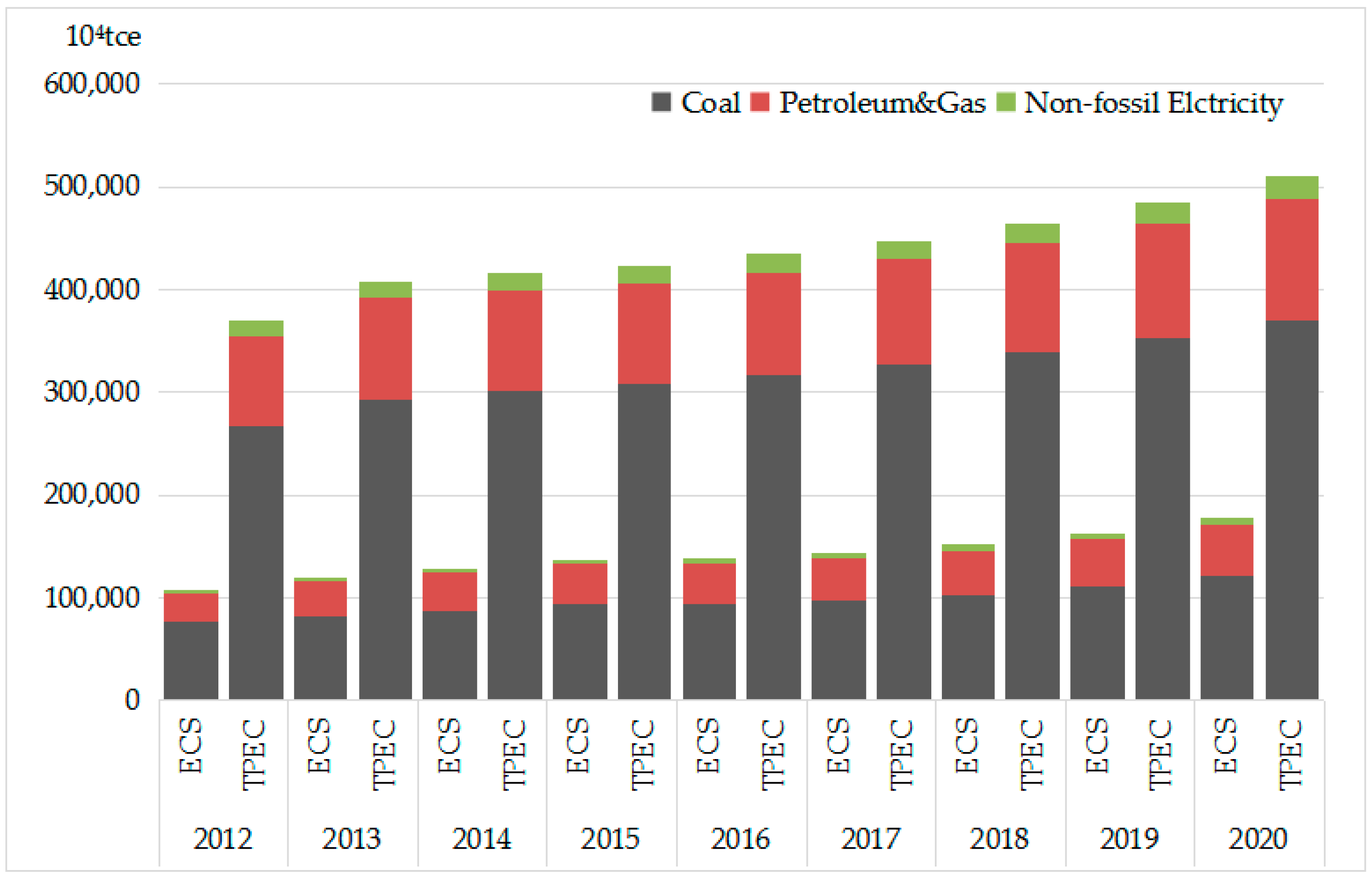
4.1. Forecast Results of Energy Consumption and EECS

According to the economic prediction in this paper, the forecast results of TPEC and EECS for China from 2012 to 2020 are shown in Figure 2.

China’s TPEC and EECS will increase until 2020. By 2020, China’s TPEC will reach 5.10 billion tons of coal equivalent (Gtce), and the EECS will reach 1.79 Gtce. The reason for the steady growth in TPEC is that China’s GDP is set to grow at a steady rate, which leads to a steady increase in the final demand of each sector. Due to the constant growth rate in GDP, the annual GDP increase will increase with time, which leads to an increasing demand for construction services and the increase in EECS.

The growth rate of EECS is higher than that of TPEC. The proportion of EECS to TPEC will rise from 29% in 2013 to 35% in 2020. To meet the economic growth rate determined in this paper, a large quantity of CSFAI will need to meet the increasing production demand of various sectors, which causes a higher growth in EECS. Based on the forecast in this paper, China’s TPEC and EECS will not automatically decrease before 2020. The contribution of EECS will increase as GDP increases at a steady rate. Therefore, controlling measures are needed to reduce EECS and TPEC. To this end, we need to understand the impact of various factors on EECS and TPEC. To verify the credibility of the forecast in this paper, the TPEC and FAI forecasts for China from 2013 to 2016 were compared with the data published by the NBS [58] of China. FAI from 2013 to 2016 is displayed by the proportion of FAI in 2012. The results of this comparison are shown in

Table 9. The comparison of the forecast and data published by National Bureau of Statistics (NBS) (billion tons of coal equivalent, Gtce).

Parameters	Specific Categories of Parameters	2013	2014	2015	2016
TPEC	Data from NBS	4.17	4.26	4.30	4.36
	Forecast of this paper	4.08	4.16	4.23	4.34
	Deviation	−2.22%	−2.36%	−1.59%	−0.33%
FAI	Data from NBS	116%	133%	145%	154%
	Forecast of this paper	116%	130%	146%	151%
	Deviation	−0.33%	−1.53%	0.63%	−2.08%

.

The comparison shows that the forecast results from this paper are close to the data published by the NBS of China: the deviation of TPEC is less than 3%, and the forecast of FAI is also basically consistent with the data published by NBS. Moreover, the TPEC of China in 2020 forecasted by the Chinese Academy of Engineering [13] is 4.8 Gtce, and the TPEC of China in 2020 forecasted by the Chinese Energy Research Institute [14] is 5.2 Gtce. The forecast results of China’s TPEC in 2020 of this paper is between the forecast results of the two institutes, which shows that the forecast results of this paper can be supported by other studies and statistical data. Therefore, the CSDHI/O model proposed in this paper can be applied to forecast TPEC and EECS.

4.2. Sensitivity Analysis of Each Influencing Factor

The factors that influence the EECS of an economy include: (1) GDP growth rate, (2) proportion of final demand of each sector, (3) fabrication level, and (4) the positive capital coefficient. Through the sensitivity analysis of these factors, we analyzed the impact of each factor on EECS and TPEC. Based on the results of sensitivity analysis and scenario analysis, we identified the key factor to conserve EECS and TPEC, and provide policy implications.

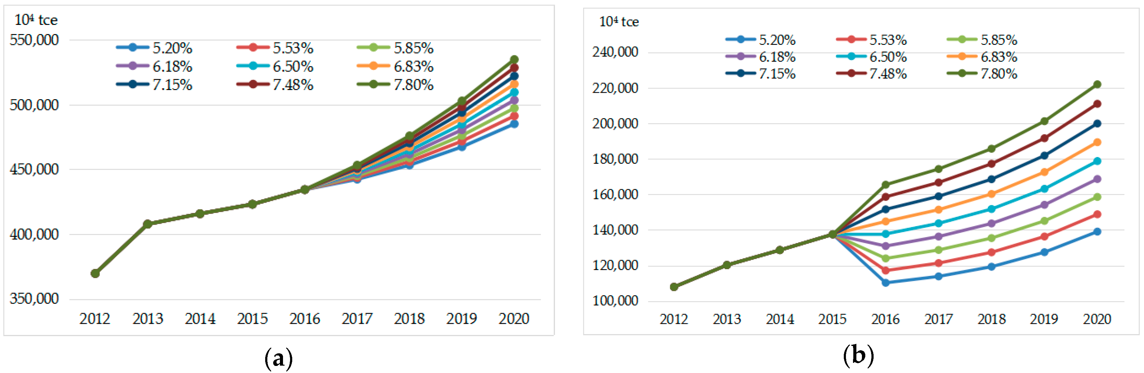
4.2.1. Sensitivity Analysis of GDP Growth Rate

Since the GDP of China from 2013 to 2016 was published by NBS [58], the published data were adopted. Since 2017, the influence of different GDP growth rates on China’s TPEC and EECS is shown in Figure 3.

With a higher GDP growth rate, China’s TPEC of each year will be larger. With the GDP growth rate fluctuating in the ±20% range (5.20–7.80%) since 2017, the TPEC in 2020 will change in the ±5% range (from 4.85 Gtce to 5.35 Gtce). The GDP growth rate will directly determine the total final demand in China, which leads to changes in the output of various sectors, thus affecting TPEC.

The EECS of each year will increase as the GDP growth rate increases. When the GDP growth rate changes ±20%, the EECS in 2020 will change from −22% to 24% (from 1.39 Gtce to 2.22 Gtce). The abrupt change in EECS in 2016 was due to the sudden change in GDP growth rate in 2017. The change in the output of each sector caused by the change in GDP growth rate leads to the change in construction services in various sectors, which results to the change in EECS in 2016.

Compared to TPEC, EECS is more sensitive to the change in GDP growth rate. When GDP growth rate decreases, the quantity of construction services decrease significantly or even completely to zero, while the quantity of total energy services also decreases, but the decline will be smaller than that of construction services. Therefore, compared to the total energy services, construction services are more sensitive to the change in GDP growth rate, and EECS is more sensitive than TPEC.

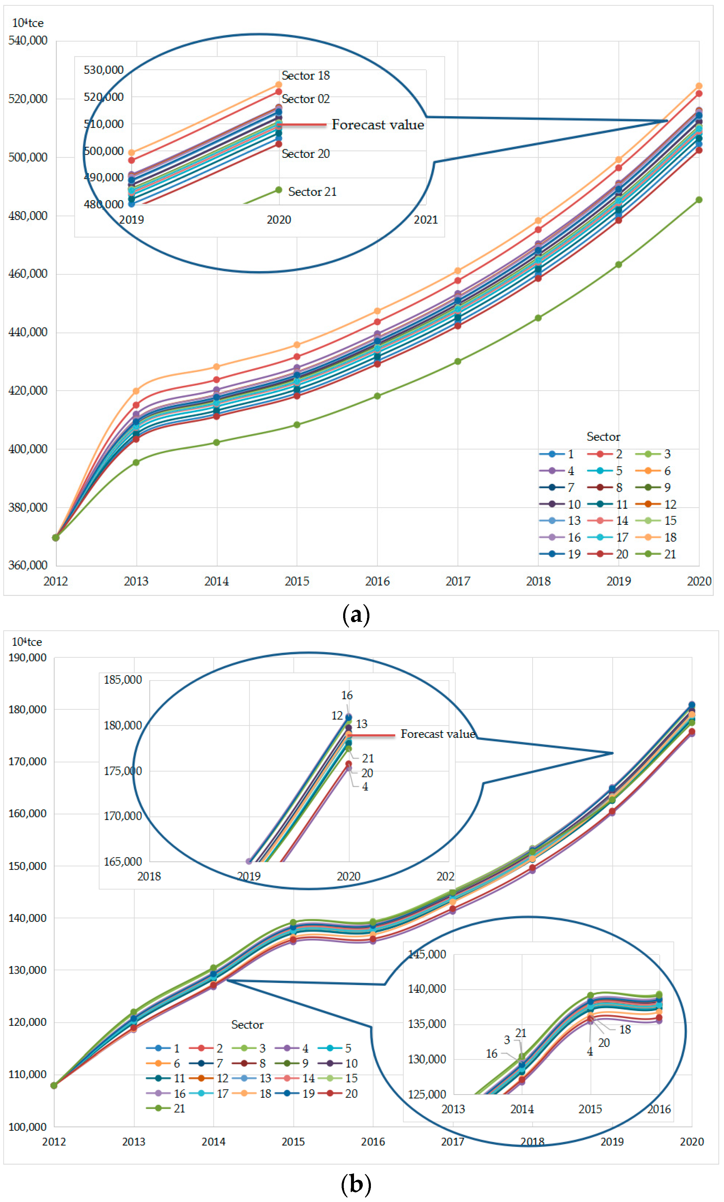
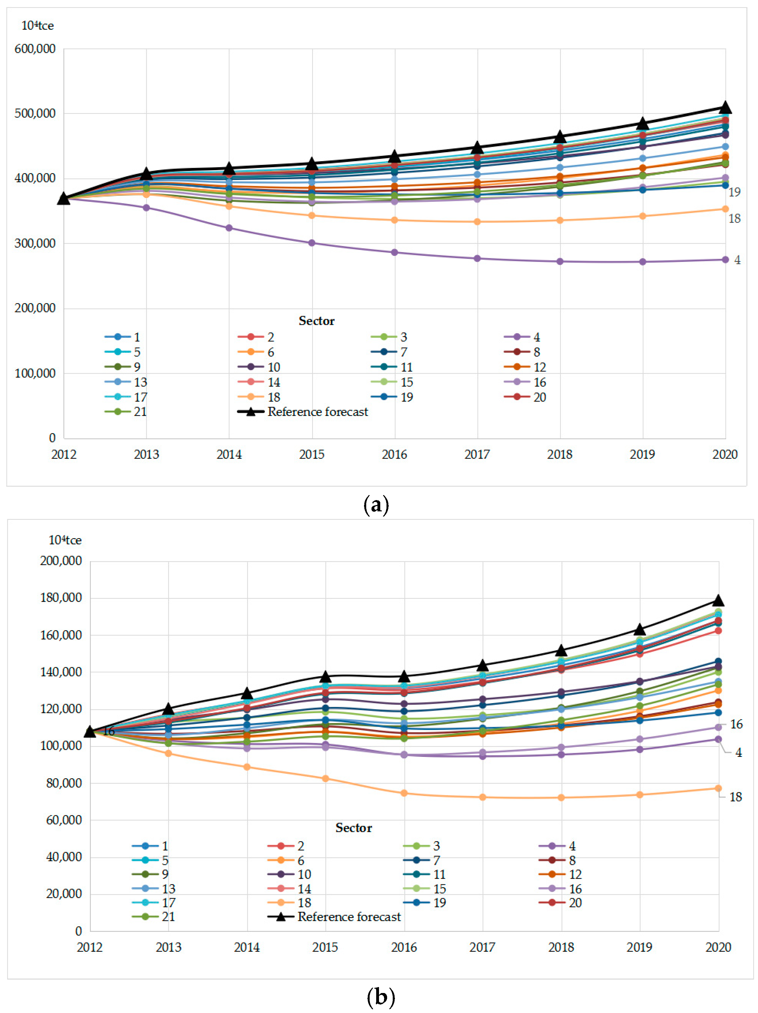
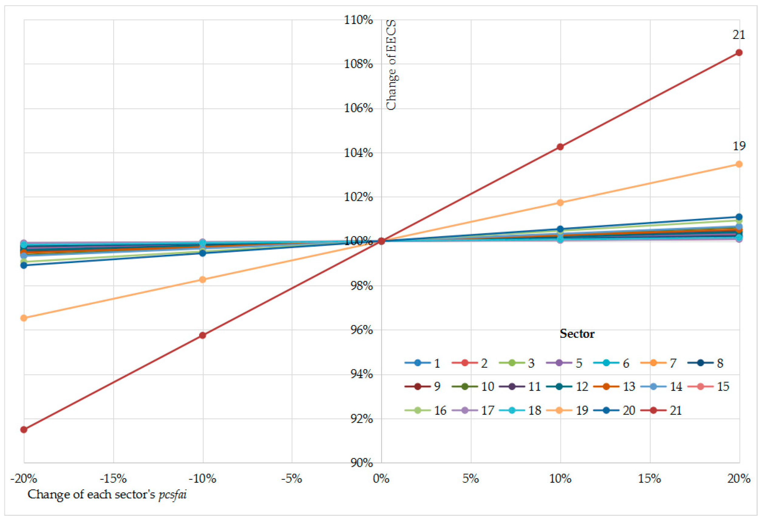
4.2.2. Sensitivity Analysis of Proportion of Final Demand

To analyze the sensitivity of the proportion of the final demand, the proportion of each sector’s final demand to the total final demand was assumed to increase by 20%. The sensitivity analysis of the proportion of the final demand of TPEC and EECS is shown in Figure 4.

The increase in the service industry’s final demand proportion has the greatest impact on the conservation of TPEC. The change in the proportion of final demand for each sector has little influence on the growth trend of TPEC. The increase in the proportion of final demand of some sectors, such as sectors in tertiary industry, results in a decrease in China’s TPEC, whereas the increase in the proportion of final demand of some sectors with high energy intensity produces the opposite result. The influence of the proportion of each sector’s final demand on TPEC was determined by the energy intensity and the quantity of final demand of the sector. Increasing the proportion of final demand of Sector 18 (Construction) leads to the greatest increase in China’s TPEC (increase of 2.9%), followed by Sector 02 (Petroleum and Natural Gas). Increasing the proportion of the final demand of Sector 21 (Other Tertiary Industry) results in the greatest decrease in China’s TPEC (decrease of 4.8%), followed by Sector 20 (Wholesale). Considering the proportion of final demand represents the industrial structure, reasonably adjusting the industrial structure is effective for TPEC conservation.

Adjusting the industrial structure has relatively less impact on EECS than on TPEC. Increasing the proportion of final demand of Sector 16 (Other Manufacture) leads to the greatest increase in China’s EECS (increase of 1.3%), followed by Sector 12 (Machinery). Increasing the proportion of the final demand of Sector 04 (Electric Power) results in the largest decrease in China’s EECS (decrease of 1.9%), followed by Sector 20 (Wholesale). Therefore, in order to reduce the EECS of China in 2020, increasing the proportion of final demand of Sectors 04 (Electric Power) and decreasing the proportion of the final demand of Sector 16 (Other Manufacture) would be the most effective.

Compared to EECS, TPEC is more sensitive to the change in each sector’s proportion of final demand. This is due to the greater difference in the energy intensity of products from different sectors than the difference in energy intensity of EECS.

The influence of the increase in the proportion of the final demand of a specific sector on the growth trend of EECS is not always the same. For example, an increase in the proportion of final products of Sector 21 (Other Tertiary Industries) from 2013 to 2015 leads to the largest increase in EECS. However, an increase in the proportion of the final demands of Sector 21 (Other Tertiary Industries) in 2020 results in EECS decreasing by 0.73%. Because the increase in the proportion of the final demand of a specific sector leads to a decrease in the proportion of other sectors, the ultimate impact of the increase in the proportion of the final demand of a specific sector on the EECS is a complex coupling of changes in construction services caused by the change in each sector’s final demand due to the assumptions in this paper.

4.2.3. Sensitivity Analysis of Fabrication Level

The S matrix in the RAS procedure reflects the fabrication level of various sectors. Each column elements of the S matrix decreased by 20% in this sensitivity analysis, which represents the fabrication level of each sector increased by 20%. The TPEC and EECS with different fabrication level of each sector are shown in Figure 5.

The improvement of fabrication level in each sector leads to a reduction in China’s TPEC. The improvement of fabrication level in Sector 04 (Electric Power) produces the greatest reduction in TPEC, which is 2.35 Gtce in 2020, or a reduction of 46.1%. This is because Sector 04 (Electric Power) consumes a huge quantity of energy, and it is an important energy producer. The improvement of fabrication level in Sector 04 (Electric Power) will lead to a higher conversion efficiency of primary energy to electricity in China, which results in higher energy efficiency and lower TPEC. The improvement of fabrication level in Sector 18 (Construction) and Sector 19 (Transport) also cause considerable energy conservation: 1.57 Gtce and 1.20 Gtce in 2020, respectively.

The improvement of fabrication level in each sector also reduces the EECS of China, and the amount of reduction is determined by the degree of the sector’s participation in the fixed assets production. The improvement of fabrication level in Sector 18 (Construction) produces the greatest reduction in EECS in 2020, which is 1.02 Gtce, or by 57%, followed by Sectors 04 (Electric Power) and 16 (Other Manufacture). Therefore, to reduce the EECS, it is most effective to hasten the improvement of fabrication level in Sectors 18 (Construction), 04 (Electric Power), and 16 (Other Manufacture). A 20% acceleration in the improvement of fabrication level in each of these three sectors could prevent further increases in EECS or even produce a decline trend.

EECS and TPEC are both sensitive to the improvement of fabrication level. The improvement of fabrication level is important for the conservation of both EECS and TPEC. However, it is difficult for a specific sector to achieve a 20% annual improvement of fabrication level. Therefore, to effectively conserve TPEC and EECS, multiple sectors need to achieve the improvement of fabrication level.

4.2.4. Sensitivity Analysis of the Positive Capital Coefficient

The positive capital coefficient does not affect TPEC. The column vector of the positive capital coefficient matrix represents the intensity of the construction services of the corresponding sectors. In the sensitivity analysis of the positive capital coefficient matrix, each column vector of the positive capital coefficient matrix was reduced by 20%, and the EECS was estimated. The result is shown in Figure 6.

In all sectors in China, the reduction in the positive capital coefficient of the sectors belonging to the tertiary industry leads to the largest reduction in EECS. The reduction of positive capital coefficient of Sector 21 (Other Tertiary Industries) caused the greatest decrease in EECS, which is a decrease of 8.5% in 2020, or 0.15 Gtce. This is followed by Sector 19 (Transport) and Sector 20 (Wholesale). The influence of the 20% reduction in the positive capital coefficient of most sectors on EECS in 2020 is less than 1%. Therefore, reducing the intensity of construction services of the tertiary industry can reduce EECS of China more efficiently.

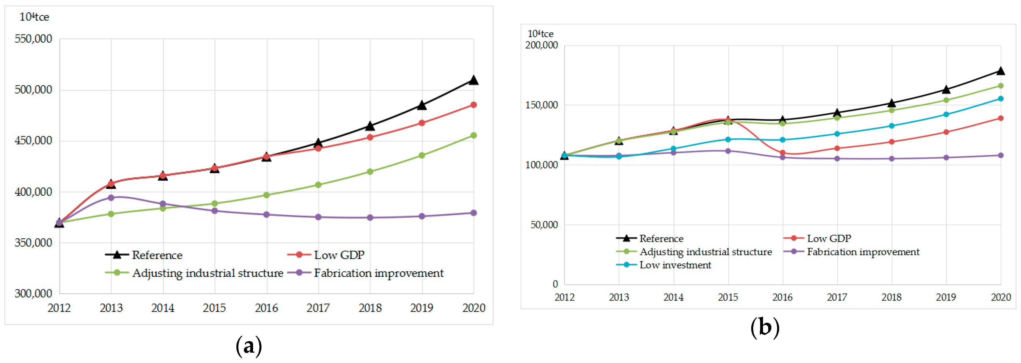
4.2.5. Comparison of Various Scenarios

Based on the results of sensitivity analysis, several scenarios were established by selecting some of the most sensitive factors to compare the influence of each factor on EECS and total energy consumption of China. The scenarios are called: (1) reference scenario, (2) low GDP scenario, (3) adjusting industrial structure scenario, (4) fabrication improvement scenario, and (5) low investment scenario:

(1)

Reference scenario: GDP growth rate, the proportion of final demand of each sector, fabrication level, and the positive capital coefficient are set as the forecast data in this paper.

(2)

Low GDP scenario: GDP growth rate after 2016 is assumed to be 20% lower than forecast in the reference scenario. Other parameter settings are the same as in the reference scenario.

(3)

Adjusting industrial structure scenario: the final demand proportion of each sector is adjusted. The final demand proportions of Sectors 02 (Petroleum and Natural Gas), 12 (Machinery), 13 (Automobiles), 16 (Other Manufacture), and 18 (Construction) are assumed to be 20% lower than the proportion of the sector in the forecast; whereas the final demand proportions of Sectors 04 (Electric Power), 20 (Wholesale), and 11 (Foods) are assumed to be 20% higher. Other parameter settings are the same as in the reference scenario.

(4)

Fabrication improvement scenario: the elements of the S matrix that represent the fabrication level of four sectors—Sectors 18 (Construction), 04 (Electric Power), 19 (Transport), and 16 (Other Manufacture)—are decreased by 2% lower than the reference scenario, which means the improvement of fabrication level in these sectors is 2% faster annually than predicted. Other parameter settings are the same as in the reference scenario.

(5)

Low investment scenario: the positive capital coefficients of Sectors 19 (Transport), 20 (Wholesale), and 21 (Other tertiary industry) are assumed to be 20% lower than in the reference scenario. Other parameter settings are the same as in the reference scenario.

TPEC and EECS of each scenario is shown in Figure 7.

In the fabrication improvement scenario, TPEC is the smallest in 2020, and remains stable after 2015. TPEC is 3.79 Gtce in 2020 in the fabrication improvement scenario, which is 25.6% lower than in the reference scenario. Only a 2% acceleration in the improvement of fabrication level in the four sectors enable China’s total energy consumption to plateau, or even decrease. A small acceleration in the improvement of fabrication level in these four sectors may be more effective than a large-scale improvement of fabrication level in one sector to reduce TPEC. In adjusting the industrial structure scenario, TPEC also decreased significantly compared with the reference scenario. In the low GDP scenario, TPEC also decreases, but with at a slower pace.

The EECS in the fabrication improvement scenario is the lowest (1.08 Gtce) in 2020, which is 39.6% lower than in the reference scenario. The EECS of China in each year is basically the same as in 2012, which shows that the EECS of China enters a plateau in the fabrication improvement scenario. The EECS in the low GDP scenario is the second lowest in 2020. A sudden decrease in GDP growth rate leads to a significant decrease in EECS, as shown in 2017. In the low investment scenario, controlling the investment in the service industry can reduce EECS by 13.1% in 2020. Adjusting the final demand proportion of various sectors has relatively little influence on EECS.

Under the scenarios in this paper, the improvement of fabrication level has the greatest impact on conservation of both TPEC and EECS in 2020 among all the influencing factors. Adjusting industrial structure is the second most effective method of conserving TPEC in China, but it is not as effective for the conservation of short-term EECS. Restricting GDP growth rate can significantly reduce EECS, but TPEC is less affected by low GDP growth rate. Decreasing the investment in service industry by, for example, improving equipment use and reducing demolition and construction waste, can reduce EECS.

4.3. Discussion

The main problem with EECS forecasting using the CSDHI/O model is whether the energy embodied in the final demands other than CSFAI can meet the consumption demand of the economy for a given year. Considering that the CSFAI estimated by the dynamic method is necessary for satisfying the hypothetical GDP growth rate, the mismatch of energy consumption with the final demands other than CSFAI and the consumption demand of the economy of the year indicates that there is a deviation in the GDP growth rate setting in the economic prediction. In order to provide energy that matches the consumption demand of the economy for the year, it is necessary to adjust the prediction of the economic growth. By adjusting the GDP growth rate and proportions of various’ final demands in the EECS forecasting, we can appropriately provide energy for the current economic demand and forecast EECS, which is essential to achieve this economic prediction.

The coefficient pcsfai affects the forecast results of EECS by affecting the CSFAI caused by the output increment of each sector. The pcsfai of all the sectors is assumed to be the same as Sector 04 (Electric Power). To verify the influence of pcsfai on the results of EECS forecasting, we made a sensitivity analysis of this coefficient. When the pcsfai of each sector fluctuates in the range of ±20% in the model, the change of the forecast results of EECS in 2020 is shown in Figure 8. The result shows that the forecast results are most sensitive to the change of pcsfai of Sector 21 (Other tertiary industry): the 20% change of pcsfai can cause 8.5% change of forecast results. However, the forecast of EECS are not sensitive to the changes of most sectors’ pcsfai. For 19 out of 21 sectors, the forecast results will change by less than 1% when pcsfai changes by 20%. Therefore, assuming pcsfai of each sector is the same as that of Sector 04 has little impact on the forecast results.

5. Conclusions and Policy Implications

A combination static and dynamic hybrid input-output model (CSDHI/O model) was developed to forecast the total primary energy consumption (TPEC) and estimate the energy consumed by construction services (EECS), which is the energy cost of economic development, based on the gross domestic product (GDP) prediction.

We used China as a case study. Based on historical Chinese data from 2007 to 2012 and economic predictions from 2013 to 2020, the EECS and TPEC were forecasted. The CSDHI/O model was effective at EECS and TPEC forecasting, and the short-term forecast was relatively close to the published data. With the sensitivity analysis of several influencing factors, including GDP growth rate, the final demand proportion of each sector, the improvement of fabrication level, and the positive capital coefficient, we analyzed the impact of each factor on EECS and TPEC. Based on the settings in this paper, the main findings are as follows: (1) the improvement of fabrication level was identified as the key factor for conserving both EECS and TPEC of China until 2020; (2) a sudden drop in GDP growth rate significantly reduces EECS, but has little effect on TPEC conservation; (3) adjusting industrial structure significantly reduces China’s TPEC, but is ineffective for the conservation of EECS; and (4) decreasing the investment in service industry also reduces EECS.

Based on results of sensitivity analysis and scenario analysis, we have the following policy recommendations: (1) hasten the improvement of fabrication level in Sectors 18 (Construction), 04 (Electric Power), 19 (Transport), and 16 (Other Manufacture) to effectively prevent the increase in EECS and TPEC in China, or even achieve a decrease; (2) speeding up the transformation of industrial structure, especially reducing the proportion of sectors with high energy intensity and increasing the proportion of sectors with low energy intensity; (3) appropriate slowdown of GDP growth, which is also the work being promoted by the Chinese government; (4) restrict the capacity expansion in service sectors.

As a next step, the CSDHI/O model can be further developed in the following directions. First, as the fixed assets may not be installed within one time series, and construction services may not be consumed only for increasing production demand of the next time series, this model can be modified into a multiple time delay model. Secondly, this model also be applied to forecast the carbon emissions and pollutant emissions caused by construction services. Finally, if more detailed data are available, we can further improve the resolution of the CSDHI/O model by more deeply analyzing the sectoral level. For example, considering the development of renewable energy power in the power sector, we can forecast the EECS, carbon emissions, and pollutant emissions for the rapid installation of various types of renewable energy power generation, if the quantities of construction services for each type of power installation can be estimated.

References

1. Ma, L.; Liu, P.; Fu, F.; Li, Z.; Ni, W. Integrated energy strategy for the sustainable development of China. Energy 2010, 36, 1143–1154. [Google Scholar] [CrossRef]
2. Fu, F.; Ma, L.; Li, Z.; Polenske, K.R. The implications of China’s investment–driven economy on its energy consumption and carbon emissions. Energy Convers. Manag. 2014, 85, 573–580. [Google Scholar] [CrossRef]
3. Li, J.S.; Xia, X.H.; Chen, G.Q.; Alsaedi, A.; Hayat, T. Optimal embodied energy abatement strategy for Beijing economy: Based on a three–scale input–output analysis. Renew. Sustain. Energy Rev. 2016, 53, 1602–1610. [Google Scholar] [CrossRef]
4. Wang, Y.; Liang, S. Carbon dioxide mitigation target of China in 2020 and key economic sectors. Energy Policy 2013, 58, 90–96. [Google Scholar] [CrossRef]
5. Pan, L.; Liu, P.; Li, Z.; Wang, Y. A dynamic input–output method for energy system modeling and analysis. Chem. Eng. Res. Des. 2018, 131, 183–192. [Google Scholar] [CrossRef]
6. Song, J.; Yang, W.; Higano, Y.; Wang, X.E. Dynamic integrated assessment of bioenergy technologies for energy production utilizing agricultural residues: An input–output approach. Appl. Energy 2015, 158, 178–189. [Google Scholar] [CrossRef]
7. Yu, S.; Zheng, S.; Ba, G.; Wei, Y.M. Can China realise its energy-savings goal by adjusting its industrial structure? Econ. Syst. Res. 2016, 28, 273–293. [Google Scholar] [CrossRef]
8. Zheng, H.; Fang, Q.; Wang, C.; Wang, H.; Ren, R. China’s Carbon Footprint Based on Input-Output Table Series: 1992–2020. Sustainability 2017, 9, 387. [Google Scholar] [CrossRef]
9. Su, B.; Ang, B.W. Structural Decomposition Analysis Applied to Energy and Emissions: Aggregation Issues. Econ. Syst. Res. 2012, 24, 299–317. [Google Scholar] [CrossRef]
10. BP. BP Energy Outlook 2017 Edition. Available online: https://www.bp.com/zh_cn/china/reports-and-publications/_bp_2017_.html (accessed on 15 November 2017).
11. BP. BP Energy Outlook 2018 Edition. Available online: https://www.bp.com/content/dam/bp/en/corporate/pdf/energy-economics/energy-outlook/bp-energy-outlook-2018.pdf (accessed on 15 November 2017).
12. International Energy Agency. World Energy Outlook 2017; International Energy Agency: Paris, France, 2017. [Google Scholar]
13. Xie, K.C.; Du, X.W.; Zhang, Y.Z.; He, J.S.; Huang, Q.L.; Yuan, Q.S.; Ni, W.D.; Jin, Y.; Cen, K.F.; Ren, X.K.; et al. Research on the Revolutionary Strategy of Promoting Energy Production and Consumption; Integrated Volume; Science Press: Beijing, China, 2017. [Google Scholar]
14. Dai, Y.D.; Tian, Z.Y.; Zhu, Y.Z.; Bai, Q.; Yang, H.W. Rebuilding Energy: China: A Road Map for Energy Consumption and Production Revolution in 2050; Integrated Volume; Science Press: Beijing, China, 2017. [Google Scholar]
15. Yu, S.; Zhu, K. A hybrid procedure for energy demand forecasting in China. Energy 2012, 37, 396–404. [Google Scholar] [CrossRef]
16. Yu, S.; Wei, Y.; Wang, K. A PSO–GA optimal model to estimate primary energy demand of China. Energy Policy 2012, 42, 329–340. [Google Scholar] [CrossRef]
17. Sözen, A.; Gülseven, Z.; Arcaklioğlu, E. Forecasting based on sectoral energy consumption of GHGs in Turkey and mitigation policies. Energy Policy 2007, 35, 6491–6505. [Google Scholar] [CrossRef]
18. Ardakani, F.J.; Ardehali, M.M. Long-term electrical energy consumption forecasting for developing and developed economies based on different optimized models and historical data types. Energy 2014, 65, 452–461. [Google Scholar] [CrossRef]
19. Pao, H.T. Forecasting energy consumption in Taiwan using hybrid nonlinear models. Energy 2009, 34, 1438–1446. [Google Scholar] [CrossRef]
20. Srinivasan, D. Energy demand prediction using GMDH networks. Neurocomputing 2008, 72, 625–629. [Google Scholar] [CrossRef]
21. Yu, S.; Wei, Y.; Wang, K. China’s primary energy demands in 2020: Predictions from an MPSO–RBF estimation model. Energy Convers. Manag. 2012, 61, 59–66. [Google Scholar] [CrossRef]
22. Xie, N.; Yuan, C.; Yang, Y. Forecasting China’s energy demand and self-sufficiency rate by grey forecasting model and Markov model. Int. J. Electr. Power Energy Syst. 2015, 66, 1–8. [Google Scholar] [CrossRef]
23. Lee, Y.; Tong, L. Forecasting energy consumption using a grey model improved by incorporating genetic programming. Energy Convers. Manag. 2011, 52, 147–152. [Google Scholar] [CrossRef]
24. Pao, H.; Fu, H.; Tseng, C. Forecasting of CO2 emissions, energy consumption and economic growth in China using an improved grey model. Energy 2012, 40, 400–409. [Google Scholar] [CrossRef]
25. Kumar, U.; Jain, V.K. Time series models (Grey-Markov, Grey Model with rolling mechanism and singular spectrum analysis) to forecast energy consumption in India. Energy 2010, 35, 1709–1716. [Google Scholar] [CrossRef]
26. Rout, U.K.; Voβ, A.; Singh, A.; Fahl, U.; Blesl, M.; Gallachóir, B.P. Energy and emissions forecast of China over a long-time horizon. Energy 2011, 36, 1–11. [Google Scholar] [CrossRef]
27. Crompton, P.; Wu, Y. Energy consumption in China: Past trends and future directions. Energy Econ. 2005, 27, 195–208. [Google Scholar] [CrossRef]
28. Yuan, C.; Liu, S.; Fang, Z. Comparison of China’s primary energy consumption forecasting by using ARIMA (the autoregressive integrated moving average) model and GM(1,1) model. Energy 2016, 100, 384–390. [Google Scholar] [CrossRef]
29. Saab, S.; Badr, E.; Nasr, G. Univariate modeling and forecasting of energy consumption: The case of electricity in Lebanon. Energy 2014, 26, 1–14. [Google Scholar] [CrossRef]
30. Chavez, S.G.; Bernat, J.X.; Coalla, H.L. Forecasting of energy production and consumption in Asturias (northern Spain). Energy 1999, 24, 183–198. [Google Scholar] [CrossRef]
31. Li, L.; Qi, P. The impact of China’s investment increase in fixed assets on ecological environment: An empirical analysis. Energy Procedia 2011, 5, 501–507. [Google Scholar] [CrossRef]
32. Acquaye, A.A.; Duffy, A.P. Input–output analysis of Irish construction sector greenhouse gas emissions. Build. Environ. 2010, 45, 784–791. [Google Scholar] [CrossRef] [Green Version]
33. Skelton, A.; Guan, D.; Peters, G.P.; Crawford-Brown, D. Mapping flows of embodied emissions in the global production system. Environ. Sci. Technol. 2011, 45, 10516–10523. [Google Scholar] [CrossRef]
34. Lenzen, M.; Dey, C.; Foran, B. Energy requirements of Sydney households. Ecol. Econ. 2004, 49, 375–399. [Google Scholar] [CrossRef] [Green Version]
35. Lenzen, M. Primary energy and greenhouse gases embodied in Australian final consumption: An input–output analysis. Energy Policy 1998, 26, 495–506. [Google Scholar] [CrossRef]
36. Cohen, C.; Lenzen, M.; Schaeffer, R. Energy requirements of households in Brazil. Energy Policy 2005, 33, 555–562. [Google Scholar] [CrossRef]
37. Liu, Z.; Geng, Y.; Lindner, S.; Zhao, H.; Fujita, T.; Guan, D. Embodied energy use in China’s industrial sectors. Energy Policy 2012, 49, 751–758. [Google Scholar] [CrossRef]
38. Liu, H.; Xi, Y.; Guo, J.E.; Li, X. Energy embodied in the international trade of China: An energy input–output analysis. Energy Policy 2010, 38, 3957–3964. [Google Scholar] [CrossRef]
39. Su, B.; Huang, H.C.; Ang, B.W.; Zhou, P. Input–output analysis of CO2 emissions embodied in trade: The effects of sector aggregation. Energy Econ. 2010, 32, 166–175. [Google Scholar] [CrossRef]
40. Zhang, Y.; Nie, R. The Energy Input-Output Model of Nine Pieces and the Demand Prediction of Jiangsu Province. Sci. Technol. Rev. 2007, 25, 25–29. [Google Scholar]
41. Hamilton, T.G.A.; Kelly, S. Low carbon energy scenarios for sub-Saharan Africa: An input-output analysis on the effects of universal energy access and economic growth. Energy Policy 2017, 105, 303–319. [Google Scholar] [CrossRef]
42. Dejuán, Ó.; Córcoles, C.; Gómez, N.; Tobarra, M.Á. Forecasting energy demand through a dynamic input-output model. Econ. Bus. Lett. 2015, 4, 108–115. [Google Scholar] [CrossRef]
43. Leontief, W. The Dynamic Inverse. In Contributions to Input-Output Analysis; Carter, A.P., Brody, A., Eds.; North Holland: Amsterdam, The Netherlands, 1970. [Google Scholar]
44. Rhoten, R.P. Dynamic input-output analysis of the economics of energy. In Proceedings of the Energy ’78. IEEE 1978 Region V Annual Conference, Tulsa, OK, USA, 16–18 April 1978. [Google Scholar]
45. Penner, P.S. A dynamic input-output analysis of net energy effects in single-fuel economies. Energy Syst. Policy 1981, 5, 89–116. [Google Scholar]
46. Dobos, I.; Tallos, P. A dynamic input-output model with renewable resources. Cent. Eur. J. Oper. Res. 2013, 21, 295–305. [Google Scholar] [CrossRef]
47. Cruz, J.B., Jr.; Tan, R.R.; Culaba, A.B.; Ballacillo, J.A. A dynamic input-output model for nascent bioenergy supply chains. Appl. Energy 2009, 861, S86–S94. [Google Scholar] [CrossRef]
48. Holz, C.A. New capital estimates for China. China Econ. Rev. 2006, 17, 142–185. [Google Scholar] [CrossRef] [Green Version]
49. Leontief, W. Environmental repercussions and the economic structure: An input–output approach. Rev. Econ. Stat. 1970, 52, 262–271. [Google Scholar] [CrossRef]
50. Guo, C.; Tang, H. Stability analysis of the dynamic input-output system. Appl. Math. A J. Chin. Univ. 2002, 17, 473–478. [Google Scholar] [CrossRef]
51. Zhou, P.; Fan, L.W.; Tang, H.W. On stability analysis of multiple objective dynamic input–output model. Appl. Math. Comput. 2006, 177, 79–84. [Google Scholar] [CrossRef]
52. Miller, R.E.; Blair, P.D. Input-Output Analysis: Foundations and Extensions; Cambridge University Press: New York, NY, USA, 2009. [Google Scholar]
53. Toh, M.H. The RAS Approach in Updating Input–Output Matrices: An Instrumental Variable Interpretation and Analysis of Structural Change. Econ. Syst. Res. 1998, 10, 63–78. [Google Scholar] [CrossRef]
54. National Bureau of Statistics. The Input-Output Table of CHINA 2007. Available online: http://data.stats.gov.cn/ifnormal.htm?u=/files/html/quickSearch/trcc/trcc01.html&h=740 (accessed on 29 December 2018).
55. National Bureau of Statistics. The Input-Output Table of CHINA 2010. Available online: http://data.stats.gov.cn/ifnormal.htm?u=/files/html/quickSearch/trcc/trcc01.html&h=740 (accessed on 29 December 2018).
56. National Bureau of Statistics. The Input-Output Table of CHINA 2012. Available online: http://data.stats.gov.cn/ifnormal.htm?u=/files/html/quickSearch/trcc/trcc01.html&h=740 (accessed on 29 December 2018).
57. National Bureau of Statistics. China Energy Statistical Yearbook 2013; China Statistics Press: Beijing, China, 2014.
58. National Bureau of Statistics. China Statistical Yearbook 2016; China Statistics Press: Beijing, China, 2017.
59. The World Bank. China Economic Update—May 2018. Available online: http://www.worldbank.org/en/country/china/publication/china-economic-update-may-2018 (accessed on 28 December 2018).
Figure 1. The combination of static and dynamic hybrid input-output (CSDHI/O) model.
Energies 12 00300 g001
Figure 2. Forecast results of the total primary energy consumption (TPEC) and energy embodied in construction services (EECS) of China.
Energies 12 00300 g002
Figure 3. Energy consumption under different GDP growth rates for (a) TPEC and (b) EECS.
Energies 12 00300 g003
Figure 4. Energy consumption in the sensitivity analysis of the proportion of final demand for (a) TPEC and (b) EECS.
Energies 12 00300 g004
Figure 5. Energy consumption in the sensitivity analysis of improvement of fabrication level: (a) TPEC and (b) EECS.
Energies 12 00300 g005
Figure 6. EECS in the sensitivity analysis of the positive capital coefficient.
Energies 12 00300 g006
Figure 7. Energy consumption in various scenarios: (a) TPEC and (b) EECS.
Energies 12 00300 g007
Figure 8. Sensitivity analysis of pcsfaii.
Energies 12 00300 g008