A Reverse Model Predictive Control Strategy for a Modular Multilevel Converter

Abstract

In recent years, modular multilevel converters (MMCs) have developed rapidly, and are widely used in medium and high voltage applications. Model predictive control (MPC) has attracted wide attention recently, and its advantages include straightforward implementation, fast dynamic response, simple system design, and easy handling of multiple objectives. The main technical challenge of the conventional MPC for MMC is the reduction of computational complexity of the cost function without the reduction of control performance of the system. Some modified MPC scan decrease the computational complexity by evaluating the number of on-state sub-modules (SMs) rather than the number of switching states. However, the computational complexity is still too high for an MMC with a huge number of SMs. A reverse MPC (R-MPC) strategy for MMC was proposed in this paper to further reduce the computational burden by calculating the number of inserted SMs directly, based on the reverse prediction of arm voltages. Thus, the computational burden was independent of the number of SMs in the arm. The control performance of the proposed R-MPC strategy was validated by Matlab/Simulink software and a down-scaled experimental prototype.

1. Introduction

Multilevel converters have been widely used in medium and high voltage applications in recent years [1,2,3]. Among various multilevel converters, the modular multilevel converter (MMC) has become more popular because of its scalability, modularity, and redundancy. An MMC can be used in many high-power applications; for example, high-voltage direct current (HVDC) systems, static synchronous compensators, grid-connected systems, and medium/high voltage motor drive systems [4,5,6].

There are some technical challenges for the control of an MMC, such as the balance of sub-module (SM) capacitor voltages, the suppression of circulating currents, and the tracking of output currents. Many control and modulation methods have been proposed to address these issues. Among them, model predictive control (MPC) is an interesting control scheme for the MMC. Its advantages include straightforward implementation, fast dynamic response, and suitability for dealing with multiple objectives [7,8,9].

Reference [10] first applied the conventional MPC scheme to MMC, in which the output currents, SM capacitor voltages, and circulating currents were controlled together by the evaluation for all the possible switching states in a cost function. In Reference [11], the proportional integral (PI) control method was experimentally compared with the conventional MPC scheme for MMC, and the conclusion was that the MPC scheme had better control performance than PI method, either for steady-state or dynamic performance. In Reference [12,13], similar methods based on conventional MPCs were used to control the MMC by evaluating for all the possible switching states of SMs. However, it is difficult to implement a conventional MPC scheme in practical applications due to the huge computation complexity because the number of all the possible switching states of SMs for an MMC with N SMs (N is the number of SMs) in each arm is as large as ${\mathrm{C}}_{2N}^N$ (e.g., MMC used for HVDC usually has more than 100 SMs, thus the number of all possible control options is more than 9 × 10⁵⁸).

In the literature, several modified strategies have been developed to reduce the computational burden [14,15,16,17,18,19,20,21,22]. Reference [14] proposed a modified method to reduce the subset of control options, which can reduce the computational burden of MPC to a certain extent. For an MMC with eight SMs per bridge, the number of switching states can be reduced to 361. In Reference [15], an integrated MPC combined with the classical energy balancing approach was proposed to reduce the number of switching states to $(N+1{)}^3$. In Reference [16], by combining with the conventional sorting algorithm, an indirect MPC was proposed to reduce the calculation burden, in which the computation complexity was determined by the SM number instead of the switching states of SMs. The number of switching states can be reduced to $(N+1{)}^2$, thus the computation complexity of indirect MPC is significantly reduced. In Reference [17], a grouping-sorting-optimized MPC strategy was proposed, in which the SMs in each arm were divided into several groups, and the computational load is determined by the number of groups and SMs of each group. The number of control options can be reduced to $2X+M+3$, where $M$ is the number of groups, and $X$ is the number of SMs in each group. Reference [18] proposed a fast MPC method, in which the number of control options could be significantly reduced to two or three by limiting the change of output voltage level in each control cycle within two or three levels near the previous output voltage level. However, the cost was the reduction of dynamic performance because the variation of the output voltage was limited in each control cycle. A dual-stage MPC scheme for MMC was proposed in Reference [19], in which the control objectives were achieved by a two-stage prediction algorithm. Compared with fast MPC method or indirect MPC method, the dual-stage MPC scheme had better dynamic performance, but the computational burden was increased. In Reference [20], a modulated MPC method combined with the sorting algorithm for MMC was proposed, in which the SMs were selected by evaluating the output voltage level and inserted at regular intervals to obtain a fixed switching frequency. The number of switching states could be reduced to $N+1$. In Reference [21], aiming at the control objectives of output currents and circulating currents, and based on evaluating the output voltage levels, the overall computation complexity of indirect MPC was reduced to $N+4$. A similar approach was also adopted in Reference [22]. However, for the MMC used in HVDC (usually with hundreds of SMs), the computational burden of indirect MPC was still too large.

In this paper, a reverse MPC (R-MPC) strategy for the MMC was proposed to further reduce computation complexity. Based on predicted output voltage of MMC, the number of control options was further reduced by calculating the number of on-state SMs directly and decoupling the SM capacitor voltage control. The control of capacitor voltage balance task was carried out in an external control loop. Thus, the computational complexity was independent of the SM number of MMC. This strategy could be used for the MMC with hundreds of SMs.

The rest of this paper is arranged as follows. Section 2 presents the topology, basic operation, and mathematical model of system. In Section 3, the details of the conventional MPC, modified MPC, and proposed R-MPC are explained. The control performance of the proposed R-MPC strategy is validated by Matlab/Simulink software and a down-scaled experimental prototype in Section 4 and Section 5, respectively. In Section 6, the conclusions are drawn.

2. Mathematical Model

The topology of the MMC and the single-phase equivalent circuit are shown in Figure 1. The MMC was comprised of three phase legs, and each leg contained an upper arm and a lower arm, which were represented by the subscript “p” and “n”, respectively. Each arm included an arm inductor $L_{\mathrm{o}}$ and $\mathrm{N}$ SMs. The arm inductor limited the $di/dt$ of the circulating currents caused by instantaneous voltage differences within the arms. The SMs usually adopted half-bridge structure, which contained two switches ($T_1$ and $T_2$) and one capacitor ($C_{\mathrm{SM}}$). The SMs generally worked in two switching states, namely, on-state and off-state. On-state: The SM output voltage was the capacitor voltage $u_{\mathrm{c}ij}$ (i = p, n, j = 1, 2, …, N) when $T_1$ was turned ON and $T_2$ was OFF. Off-state: The output voltage of the SM is zero when $T_1$ was turned OFF and $T_2$ was ON. The switching states of SMs could be written as follows:

$$S_{ij}=\{\begin{array}{ll}1,\hfill & T_1\mathrm{is}\mathrm{ON},T_2\mathrm{is}\mathrm{OFF}\hfill \\ 0,\hfill & T_1\mathrm{is}\mathrm{ON},T_2\mathrm{is}\mathrm{OFF}\hfill \end{array}$$

(1)

The capacitor voltage dynamic equation for each SM of the MMC is expressed as follows:

$$\frac{d{u}_{\mathrm{c}ij}}{dt}=i_{\mathrm{c}ij}/C_{\mathrm{SM}}$$

(2)

where $i_{\mathrm{c}ij}$ is the capacitor current, which can be obtained from the switching state $S_{ij}$ and the arm current $i_i$ as follows:

$$i_{\mathrm{c}ij}=S_{ij}{i}_i$$

(3)

Based on Figure 1, the arm current $i_{\mathrm{p}}$ and $i_{\mathrm{n}}$ can be written as follows:

$$\{\begin{array}{l}{i}_{\mathrm{p}}=\frac{1}{2}{i}_{\mathrm{o}}+i_{\mathrm{diff}}\hfill \\ i_{\mathrm{n}}=-\frac{1}{2}{i}_{\mathrm{o}}+i_{\mathrm{diff}}\hfill \end{array}$$

(4)

where $i_{\mathrm{diff}}$ is the circulating current, $i_{\mathrm{o}}$ is the output current, and they can be calculated by:

$$\{\begin{array}{l}{i}_{\mathrm{o}}=i_{\mathrm{p}}-i_{\mathrm{n}}\hfill \\ i_{\mathrm{diff}}=\frac{1}{2}(i_{\mathrm{p}}+i_{\mathrm{n}})\hfill \end{array}$$

(5)

Similarly, the arm voltage equations are as follows:

$$\{\begin{array}{l}\frac{U_{\mathrm{dc}}}{2}=u_{\mathrm{p}}+L_{\mathrm{o}}\frac{d{i}_{\mathrm{p}}}{dt}+R{i}_{\mathrm{o}}+L\frac{d{i}_{\mathrm{o}}}{dt}+e\hfill \\ \frac{U_{\mathrm{dc}}}{2}=u_{\mathrm{n}}+L_{\mathrm{o}}\frac{d{i}_{\mathrm{n}}}{dt}-R{i}_{\mathrm{o}}-L\frac{d{i}_{\mathrm{o}}}{dt}-e\hfill \end{array}$$

(6)

where $u_{\mathrm{p}}$ is the voltage of upper arm, $u_{\mathrm{n}}$ is the voltage of lower arm, $U_{\mathrm{dc}}$ is the voltage of dc link, $e$ is the voltage of grid, $L_{\mathrm{o}}$ represents the arm inductance, and $R$ and $L$ represent the equivalent resistance and inductance of the load circuit.

Based on Equations (4)–(6), the dynamic equation of the MMC can be obtained as:

$$\{\begin{array}{l}\frac{d{i}_{\mathrm{o}}}{dt}=\frac{u_{\mathrm{n}}-u_{\mathrm{p}}-2R{i}_{\mathrm{o}}-2e}{L_{\mathrm{o}}+2L}\hfill \\ \frac{d{i}_{\mathrm{diff}}}{dt}=\frac{U_{\mathrm{dc}}-(u_{\mathrm{n}}+u_{\mathrm{p}})}{2L_{\mathrm{o}}}\hfill \end{array}$$

(7)

Equation (7) indicates that the output current and the circulating current can be regulated directly by the voltage difference and voltage summation between the lower arm voltage $u_{\mathrm{n}}$ and upper arm voltage $u_{\mathrm{p}}$, respectively.

3. MPC Strategy

3.1. Conventional MPC

In general, there are three control targets for conventional MPC used for MMCs. The first control target is the balancing of SM capacitor voltages. The second control target is the tracking of output current correctly, including magnitude, frequency, and phase angle. The third control target is the suppressing of circulating current, removing its AC component and only keeping its DC component.

The discrete-time model of MPC can be obtained by the following forward Euler approximation equation:

$$\frac{dx}{dt}=\frac{x(k+1)-x(k)}{T_{\mathrm{s}}}$$

(8)

where $x$ is the variable of control objectives, $x(k+1)$, $x(k)$ are the variable values at time $k+1$ and $k$, respectively, and $T_{\mathrm{s}}$ is the sampling period.

The discrete-time dynamic models of the SM capacitor voltages, output currents, and circulating currents can be obtained as follows:

$$u_{\mathrm{c}ij}(k+1)=u_{\mathrm{c}ij}(k)+\frac{S_{ij}{i}_i(k)T_{\mathrm{s}}}{C_{\mathrm{SM}}}$$

(9)

$$i_{\mathrm{o}}(k+1)=(1-\frac{2R{T}_{\mathrm{s}}}{L_{\mathrm{o}}+2L})i_{\mathrm{o}}(k)+\frac{[u_{\mathrm{n}}(k)-u_{\mathrm{p}}(k)-2e(k)]T_{\mathrm{s}}}{L_{\mathrm{o}}+2L}$$

(10)

$$i_{\mathrm{diff}}(k+1)=i_{\mathrm{diff}}(k)+\frac{[U_{\mathrm{dc}}-u_{\mathrm{n}}(k)-u_{\mathrm{p}}(k)]T_{\mathrm{s}}}{2L_{\mathrm{o}}}$$

(11)

For MMC, the balancing of SM capacitor voltages, tracking of output current, and suppressing of circulating current should be achieved simultaneously. Because these control variables (SM capacitor voltages, output currents, circulating currents) interact with each other, they can be included in a multivariable cost function with weighting factors. More details of the MPC cost function can be found in [10,11,12]. The cost function can be defined as follows:

$$g={\lambda }_1\left|i_{\mathrm{o}}^{*}(k+1)-i_{\mathrm{o}}^{\mathrm{p}}(k+1)\right|+{\lambda }_2\left|i_{\mathrm{diff}}^{*}(k+1)-i_{\mathrm{diff}}^{\mathrm{p}}(k+1)\right|+{\lambda }_3\left|U_{dc}/N-u_{\mathrm{c}ij}^{\mathrm{p}}(k+1)\right|$$

(12)

where ${\lambda }_1$, ${\lambda }_2$, and ${\lambda }_3$ are the function weighing factors, $i_{\mathrm{o}}^{*}(k+1)$, $i_{\mathrm{diff}}^{*}(k+1)$, $U_{dc}/N$ are the reference values of control objectives, and $i_{\mathrm{o}}^{\mathrm{p}}(k+1)$, $i_{\mathrm{diff}}^{\mathrm{p}}(k+1)$, and $u_{\mathrm{c}ij}^{\mathrm{p}}(k+1)$ are the next-step predicted values of control objectives, respectively.

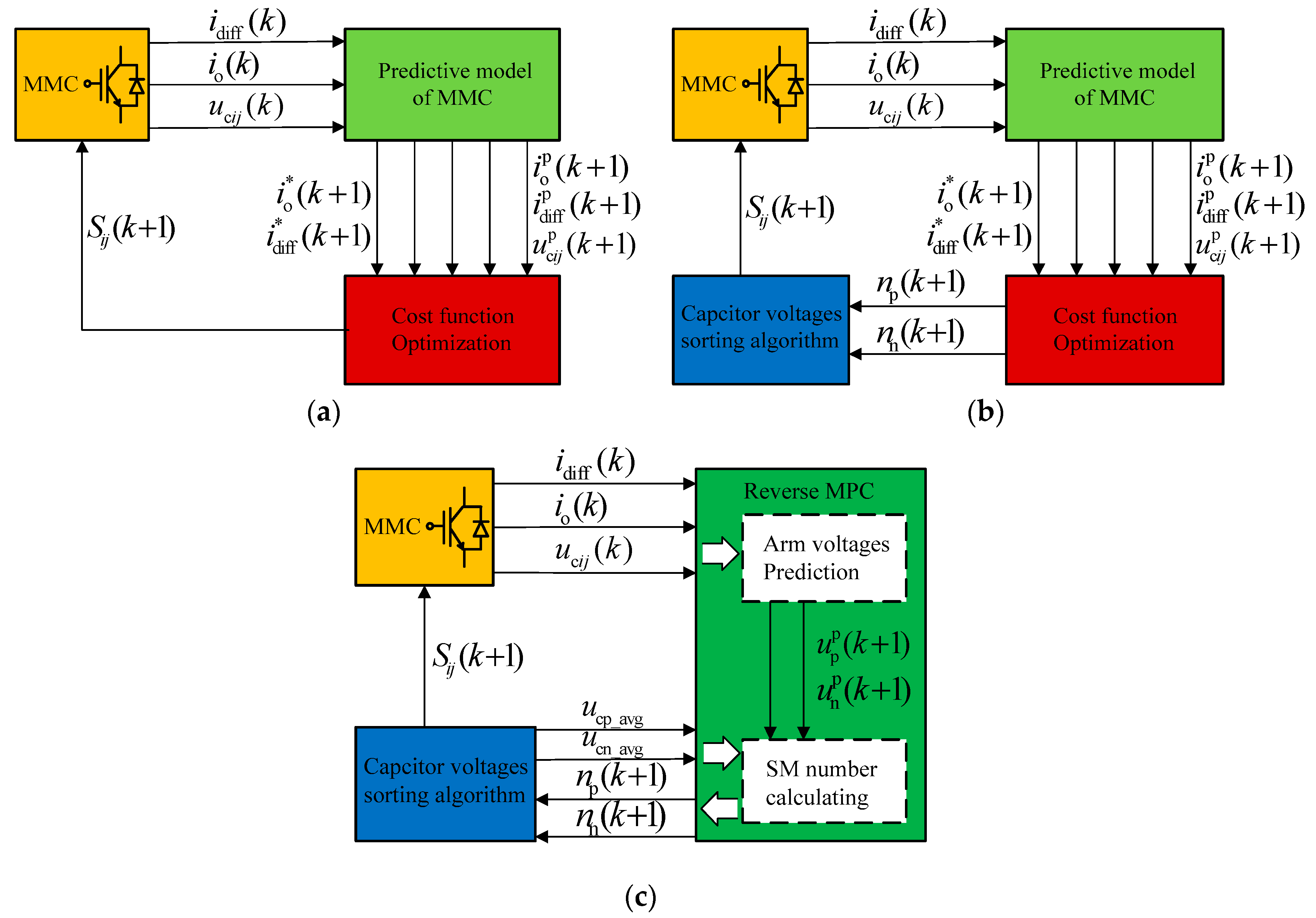
The block diagram of conventional MPC is shown in Figure 2a. Within each sampling period of MPC strategy, the cost function was evaluated one step ahead, and the switching state that minimized the cost function was chosen and used to control the converter at next switching cycle by evaluating for all the possible switching states of the converter.

Nevertheless, the number of all possible switching states for an MMC with N SMs in each bridge is ${\mathrm{C}}_{2N}^N$. For example, an MMC used for HVDC usually has more than 100 SMs per arm, thus the number of all possible switching states in one phase is more than 9 × 10⁵⁸. Therefore, it is challenging to implement the conventional MPC by the existing digital processors in practical applications due to large computation load.

3.2. Modified MPC

Some modified MPC strategies have been developed to reduce the computational burden. In combination with decoupling the SM capacitor voltage control and carrying it out in an independent control loop, indirect MPC [16,21] (shown in Figure 2b) can be used to reduce the computation complexity by evaluating the number of inserted SMs instead of the all possible switching states. However, the computational burden is still too high when the MMC has huge number of SMs.

In addition, the fast MPC [18] method can significantly reduce the computational burden to two or three by limiting the change of output voltage level in every control cycle within two or three levels near the previous output voltage level. However, the cost would be the reduction of dynamic performance because the variation of the output voltage was limited in each control cycle.

3.3. Reverse MPC

Figure 2c shows the reverse MPC (R-MPC) strategy, which was proposed to further reduce the computational complexity of MPC by decoupling the SM capacitor voltage control and carrying it out in an independent control loop. Assuming the on-state SM numbers of the upper arm and lower arm at next step are $n_{\mathrm{p}}$ and $n_{\mathrm{n}}$, the SM capacitor voltages should be resorted in either ascending or descending order, according to the direction of the corresponding arm current. $n_i(i=\mathrm{p},\mathrm{n})$ SMs with the lowest voltages are chosen to be inserted to the arm when the arm current is positive, and the other SMs are bypassed. On the contrary, $n_i(i=\mathrm{p},\mathrm{n})$ SMs with the highest voltages are selected to be inserted to the arm when the arm current is negative, and the other SMs are bypassed.

The balancing of SM capacitor voltage is one of key issues in MMC. The modified MPC generally uses the conventional sorting method (e.g., bubble sorting) to balance the SM capacitor voltages [16,18,20,22], in which all of the SM capacitor voltages have to be sorted in ascending or descending order to determine the inserted SMs with the highest or lowest voltages. However, the sorting algorithm itself is not a trivial task when MMC has huge number of SMs. Therefore, many improved sorting methods were presented to reduce the computational complexity, such as grouping sorting method [17], fundamental-frequency sorting method [23], limited sorting method [24], etc. In general, as long as several SMs with the highest or lowest voltages are selected, the voltage balance task can be completed within an allowable range of voltages ripples, while the rest SMs need not be sorted to reduce the computational burden. In addition, using the parallel computing method, FPGA (Field Programmable Gate Array) can be used to complete the SM capacitor voltage balancing task more quickly, which does not occupy CPU resources [9,16].

After the sorting task, assuming all of the capacitor voltages are balanced well, then the number of on-state SMs for upper arm and lower arm at next-step can be calculated if the next-step arm voltage can be predicted.

From Equation (7), the arm voltages can be written as follows:

$$\{\begin{array}{l}{u}_{\mathrm{p}}=\frac{U_{\mathrm{dc}}}{2}-L_{\mathrm{o}}\frac{d{i}_{\mathrm{diff}}}{dt}-(\frac{L_{\mathrm{o}}}{2}+L)\frac{d{i}_{\mathrm{o}}}{dt}-R{i}_{\mathrm{o}}-e\hfill \\ u_{\mathrm{n}}=\frac{U_{\mathrm{dc}}}{2}-L_{\mathrm{o}}\frac{d{i}_{\mathrm{diff}}}{dt}+(\frac{L_{\mathrm{o}}}{2}+L)\frac{d{i}_{\mathrm{o}}}{dt}+R{i}_{\mathrm{o}}+e\hfill \end{array}$$

(13)

By using the backward Euler approximation,

$$\frac{dx}{dt}=\frac{x(k)-x(k-1)}{T_{\mathrm{s}}}$$

(14)

The discrete-time dynamic models of the arm voltages of MMC can be written as follows:

$$\{\begin{array}{l}{u}_{\mathrm{p}}(k)=\frac{U_{\mathrm{dc}}}{2}-\frac{L_{\mathrm{o}}}{T_{\mathrm{s}}}[i_{\mathrm{diff}}(k)-i_{\mathrm{diff}}(k-1)]-(\frac{L_{\mathrm{o}}/2+L}{T_{\mathrm{s}}}+R)i_{\mathrm{o}}(k)+\frac{L_{\mathrm{o}}/2+L}{T_{\mathrm{s}}}{i}_{\mathrm{o}}(k-1)-e(k)\hfill \\ u_{\mathrm{n}}(k)=\frac{U_{\mathrm{dc}}}{2}-\frac{L_{\mathrm{o}}}{T_{\mathrm{s}}}[i_{\mathrm{diff}}(k)-i_{\mathrm{diff}}(k-1)]+(\frac{L_{\mathrm{o}}/2+L}{T_{\mathrm{s}}}+R)i_{\mathrm{o}}(k)-\frac{L_{\mathrm{o}}/2+L}{T_{\mathrm{s}}}{i}_{\mathrm{o}}(k-1)+e(k)\hfill \end{array}$$

(15)

Assuming the next-step reference values of control objectives can be tracked without error, thus, the next-step predicted arm voltages $u_{\mathrm{p}}^{\mathrm{p}}(k+1)$ and $u_{\mathrm{n}}^{\mathrm{p}}(k+1)$ can be obtained by shifting forward (Equation (15)), as follows:

$$\{\begin{array}{l}{u}_{\mathrm{p}}^{\mathrm{p}}(k+1)=\frac{U_{\mathrm{dc}}}{2}-\frac{L_{\mathrm{o}}}{T_{\mathrm{s}}}[i_{\mathrm{diff}}^{*}(k+1)-i_{\mathrm{diff}}(k)]-(\frac{L_{\mathrm{o}}/2+L}{T_{\mathrm{s}}}+R)i_{\mathrm{o}}^{*}(k+1)+\frac{L_{\mathrm{o}}/2+L}{T_{\mathrm{s}}}{i}_{\mathrm{o}}(k)-e^{*}(k+1)\hfill \\ u_{\mathrm{n}}^{\mathrm{p}}(k+1)=\frac{U_{\mathrm{dc}}}{2}-\frac{L_{\mathrm{o}}}{T_{\mathrm{s}}}[i_{\mathrm{diff}}^{*}(k+1)-i_{\mathrm{diff}}(k)]+(\frac{L_{\mathrm{o}}/2+L}{T_{\mathrm{s}}}+R)i_{\mathrm{o}}^{*}(k+1)-\frac{L_{\mathrm{o}}/2+L}{T_{\mathrm{s}}}{i}_{\mathrm{o}}(k)+e^{*}(k+1)\hfill \end{array}$$

(16)

where $i_{\mathrm{diff}}^{*}(k+1)$ is the next-step reference value of circulating current, $i_{\mathrm{o}}^{*}(k+1)$ is the next-step reference value of output current, and $e^{*}(k+1)$ is the next-step reference values of grid voltage.

For the circulating current, the main frequency component is DC, its next-step reference value $i_{\mathrm{diff}}^{*}(k+1)$ can be replaced by the previous reference value $i_{\mathrm{diff}}^{*}(k)$. But for output current and grid voltage, in order to improve the control accuracy, the next-step reference value $i_{\mathrm{o}}^{*}(k+1)$, $e^{*}(k)$ can be predicted by the formula of the Lagrange extrapolation [25], as follows:

$$i_{\mathrm{o}}^{*}(k+1)=3i_{\mathrm{o}}^{*}(k)-3i_{\mathrm{o}}^{*}(k-1)+i_{\mathrm{o}}^{*}(k-2)$$

(17)

$$e^{*}(k+1)=3e^{*}(k)-3e^{*}(k-1)+e^{*}(k-2)$$

(18)

At last, the number of next-step on-state SMs can be calculated as follows:

$$\{\begin{array}{l}{n}_{\mathrm{p}}^{\mathrm{p}}(k+1)=\mathrm{round}(\frac{u_{\mathrm{p}}^{\mathrm{p}}(k+1)}{u_{\mathrm{cp}\_\mathrm{avg}}(k)})\hfill \\ n_{\mathrm{n}}^{\mathrm{p}}(k+1)=\mathrm{round}(\frac{u_{\mathrm{n}}^{\mathrm{p}}(k+1)}{u_{\mathrm{cn}\_\mathrm{avg}}(k)})\hfill \end{array}$$

(19)

where $u_{\mathrm{cp}\_\mathrm{avg}}(k)$ and $u_{\mathrm{cn}\_\mathrm{avg}}(k)$ are the average arm voltages of the MMC (upper arm and lower arm).

The number of control options of the proposed R-MPC strategy was further reduced to one by calculating the number of on-state SMs directly based on the reverse prediction of arm voltages. Thus, the computational burden was independent of the number of SMs in the arm. This strategy was especially suitable for the MMC which has huge number of SMs. The number of control options for different MPC strategies are listed in

Table 1. Number of control options of different MPC strategies.

Number of SM (N)		4	10	50	100	200
Number of control options	Conventional MPC [10,11,12,13]	70	1.8 × 105	1.0 × 1029	9.1 × 1058	1.0 × 10119
	Integrated MPC [15]	125	1331	1.3 × 105	1.0 × 106	8.1 × 106
	Indirect MPC-I [16]	25	121	2601	1.0 × 104	4.0 × 104
	Indirect MPC-II [21]	8	14	54	104	204
	Modulated MPC [20]	5	11	51	101	201
	Indirect MPC-III [22]	5	11	51	101	201
	Fast MPC [18]	2~3	2~3	2~3	2~3	2~3
	Proposed MPC (R-MPC)	1	1	1	1	1

. As can be seen from this table, fast MPC and proposed R-MPC have the least computational complexity, especially for the MMC with hundreds of SMs.

It should be noted that the computational burden of R-MPC is independent of the number of SMs, but the computational burden of sorting algorithm is still related to the number of SMs. However, the sorting algorithm can be improved by other means [9,16,17,23,24] to reduce its computational load.

4. Simulation Results

As shown in Figure 1, a three-phase MMC system was investigated in MATLAB/Simulink softwareto validate the control performance of the proposed R-MPC strategy.

Table 2. Parameters of MMC system.

Parameter	Simulation	Experiment
Rated power (kVA)	5000	2
Rated line voltage (V)	10,000	200
DC bus voltages (V)	20,000	400
SMs per arm	32	8
SM capacitance (μF)	4700	1000
SM capacitor voltage (V)	625	50
Arm buffer inductance (mH)	2.8	2.8
Load inductance (mH)	1	1
Load resistance (Ω)	0.01	1.6
Output frequency (Hz)	50	50
Sampling period (μs)	100	100

lists the parameters of the MMC.

4.1. Steady-State Operation

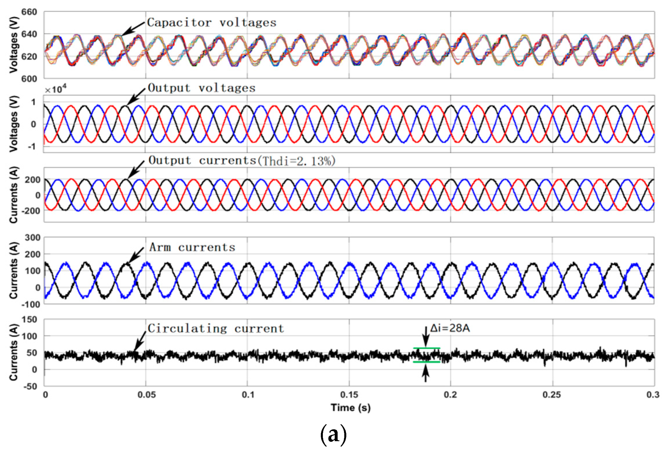
Figure 3 shows the steady-state operation results of a fast MPC [18], an indirect MPC [21], and the proposed R-MPC strategy, respectively. Three MPC strategies have almost the same steady state performance. All the capacitor voltages are well balanced, which are around 3% of their rated values. All the circulating currents are also well-suppressed, with peak-peak ripple values of 28 A, 20 A and 26 A, respectively. The total harmonic distortions (THD) of output currents are only 2.13%, 2.43%, and 2.02%, respectively. The results show that the three strategies all had good steady-state performance. But for an MMC with hundreds of SMs, fast MPC and R-MPC have more advantages because of less computational burden.

Figure 4 shows the harmonic spectrums of the output voltages and currents with proposed R-MPC. The THDs of output voltages and currents were only 1.88% and 2.02%, respectively. The results showed that the low-order harmonics were very small and within acceptable range. Thus, the noises generated by prediction did not affect the quality of the generated voltages/currents.

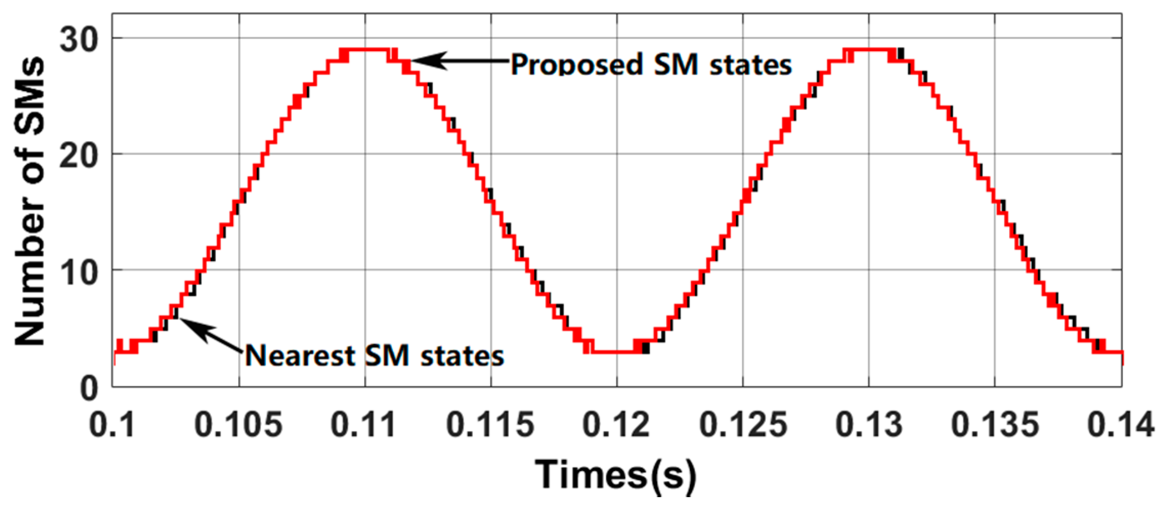
Figure 5 shows the comparison of output SM states between the traditional nearest level modulation (NLM) method and the R-MPC strategy proposed in this paper. The NLM method just obtains the nearest level state from the reference voltage, according to the tracking of output currents, however, R-MPC strategy considers not only the tracking of output current but also the suppressing of circulating current and the system delay compensation. Thus, the two methods generated different SM states and switching sequences.

4.2. Dynamic Operation

Figure 6 shows the step response results of fast MPC [18], an indirect MPC [21], and the proposed R-MPC strategy, respectively. Before t = 0.1 s, the MMC system reached a stable state, after which the magnitudes of the reference output currents experienced two step changes, stepped up from 100 A to 200 A at t = 0.1 s and stepped down from 200 A to 100 A at t = 0.2 s. In Figure 6b,c the capacitor voltages were well balanced after the step changes, the output currents of the indirect MPC and the proposed R-MPC could rapidly track their references, and the circulating currents were still well-suppressed. However, as seen in Figure 6a the output currents of the fast MPC took more time to reach the references because the change of output voltage level in each control cycle was limited within two or three levels near the previous output voltage level.

The results showed that the indirect MPC and the proposed R-MPC both had better dynamic-state performance than the fast MPC. However, for the MMC with hundreds of SMs, the R-MPC had more advantages due to less computational burden.

5. Experimental Results

Figure 7 shows a down-scaled experimental prototype of the MMC (2 kVA), setup to verify the control performance of the proposed R-MPC.A DSP/FPGA-based central control board was chosen to complete the control scheme. The DSP (TI TMS320F28335) was used for mathematical calculations and the MPC algorithm. The FPGA (Altera EP2C8Q208C8) was used for Pulse-width modulation (PWM) generation, the sorting algorithm of capacitor voltages, and fault protection. Table 2 lists the parameters of the experimental prototype.

It should be noted that a larger load resistance than that of simulation was chosen because the experimental prototype could only operate in the passive inversion state (limited by the experimental conditions), but the simulation model operated in the active inversion state, which simulated the working characteristics of HVDC. In addition, also limited by the experimental conditions, the SM capacitance was also smaller than that of simulation, which would increase the capacitor voltage ripple slightly. Despite the above differences in load and capacitor parameters, it would not affect the performance comparison and analysis of different control strategies.

5.1. Steady-State Operation

Figure 8 gives the steady-state experimental results of fast MPC [18], an indirect MPC [21], and the proposed R-MPC strategy, respectively. As seen in Figure 8, three MPC strategies had almost the same steady state performance, where the total harmonic distortions (THD) of output currents were 5.1%, 5.4%, and 5.0%, respectively. In addition, the capacitor voltages of the MMC were well-balanced and the circulating currents were also well-suppressed. The results showed that the three strategies all had good steady-state performance. But, for MMC with hundreds of SMs, fast MPC and R-MPC had more advantages because of less computational burden.

5.2. Dynamic Operation

Figure 9 shows the step response results of fast MPC [18], an indirect MPC [21], and the proposed R-MPC strategy, respectively. Before t = 1.2 s, the MMC system reached a stable state, after which the magnitudes of the reference output currents experienced one step change, stepped up from 2 A to 4 A. From Figure 9b,c it is easy to see that the capacitor voltages could be balanced well after step changes, the circulating currents were well-suppressed, and the output currents could be rapidly tracked to their references, for both indirect MPC and proposed R-MPC strategy. However, as seen in Figure 9a, the output currents of the fast MPC took more time to reach the references because the change of output voltage level in each control cycle was limited within two or three levels near the previous output voltage level.

The results show that the indirect MPC and proposed R-MPC both have better dynamic-state performance than the fast MPC. However, for MMC with hundreds of SMs, the R-MPC have more advantages due to less computational burden.

6. Conclusions

In order to reduce the computational complexity of MPC for MMC, this paper proposed a R-MPC strategy. Compared with the fast MPC and indirect MPC, the number of control options to be calculated of proposed R-MPC was greatly reduced to one by calculating the number of on-state SMs directly based on the reverse prediction of arm voltages. The simulation and experimental results of steady-state operation showed that the fast MPC, an indirect MPC, and the proposed R-MPC all had good steady-state performance, but fast MPC and the proposed R-MPC had more advantages than indirect MPC because of less computational burden. However, the simulation and experimental results of dynamic operation showed that the proposed R-MPC had better dynamic-state performance than the fast MPC. Therefore, the proposed R-MPC strategy would be especially suitable for an MMC with hundreds of SMs because of less computational burden and good performance of both steady-state and dynamic operation.

References

- Dekka, A.; Wu, B.; Fuentes, L.R.; Perez, M.; Zargari, R.N. Evolution of Topologies, Modeling, Control Schemes, and Applications of Modular Multilevel Converters. IEEE J. Emerg. Sel. Top. Power Electron. 2017, 5, 1631–1656. [Google Scholar] [CrossRef]
- Grandi, G.; Loncarski, J.; Dordevic, O. Analysis and Comparison of Peak-to-Peak Current Ripple in Two-Level and Multilevel PWM Inverters. IEEE Trans. Ind. Electron. 2015, 62, 2721–2730. [Google Scholar] [CrossRef] [Green Version]
- Zhetessov, A.; Ruderman, A. Time-domain optimization of current THD for a single-phase three-level inverter modulation. In Proceedings of the 19th International Conference on Electrical Drives and Power Electronics (EDPE), Dubrovnik, Croatia, 4–6 October 2017; pp. 82–87. [Google Scholar] [CrossRef]
- He, L.; Zhang, K.; Xiong, J.; Fan, S. A Repetitive Control Scheme for Harmonic Suppression of Circulating Current in Modular Multilevel Converters. IEEE Trans. Power Electron. 2015, 30, 471–481. [Google Scholar] [CrossRef]
- Zhang, M.; Huang, L.; Yao, W.; Lu, Z. Circulating Harmonic Current Elimination of a CPS-PWM-Based Modular Multilevel Converter with a Plug-In Repetitive Controller. IEEE Trans. Power Electron. 2014, 29, 2083–2097. [Google Scholar] [CrossRef]
- Zeng, R.; Xu, L.; Yao, L.; Finney, J.S.; Wang, Y. Hybrid HVDC for Integrating Wind Farms with Special Consideration on Commutation Failure. IEEE Trans. Power Deliv. 2016, 31, 789–797. [Google Scholar] [CrossRef]
- Dekka, A.; Wu, B.; Yaramasu, V.; Fuentes, L.R.; Zargari, R.N. Model Predictive Control of High-Power Modular Multilevel Converters–An Overview. IEEE J. Emerg. Sel. Top. Power Electron. 2018. (Early Access). [Google Scholar] [CrossRef]
- Leuer, M.; Lönneker, M.; Böcker, J. Model predictive control strategy for multi-phase thyristor matrix converters—Advantages, problems and solutions. In Proceedings of the 18th European Conference on Power Electronics and Applications (EPE’16 ECCE Europe), Karlsruhe, Germany, 6–8 September 2016; pp. 1–10. [Google Scholar] [CrossRef]
- Guo, P.; He, Z.; Yue, Y.; Xu, Q.; Huang, X.; Chen, Y.; Luo, A. A Novel Two-Stage Model Predictive Control for Modular Multilevel Converter with Reduced Computation. IEEE Trans. Ind. Electron. 2019, 66, 2410–2422. [Google Scholar] [CrossRef]
- Qin, J.; Saeedifard, M. Predictive Control of a Modular Multilevel Converter for a Back-to-Back HVDC System. IEEE Trans. Power Deliv. 2012, 27, 1538–1547. [Google Scholar] [CrossRef]
- Böcker, J.; Freudenberg, B.; The, A.; Dieckerhoff, S. Experimental Comparison of Model Predictive Control and Cascaded Control of the Modular Multilevel Converter. IEEE Trans. Power Electron. 2015, 30, 422–430. [Google Scholar] [CrossRef]
- Dekka, A.; Wu, B.; Yaramasu, V.; Zargari, R.N. Model Predictive Control With Common-Mode Voltage Injection for Modular Multilevel Converter. IEEE Trans. Power Electron. 2017, 32, 1767–1778. [Google Scholar] [CrossRef]
- Zhou, D.; Yang, S.; Tang, Y. A Voltage-Based Open-Circuit Fault Detection and Isolation Approach for Modular Multilevel Converters with Model-Predictive Control. IEEE Trans. Power Electron. 2018, 33, 9866–9874. [Google Scholar] [CrossRef]
- Perez, A.M.; Rodriguez, J.; Fuentes, J.E.; Kammerer, F. Predictive Control of AC–AC Modular Multilevel Converters. IEEE Trans. Ind. Electron. 2012, 59, 2832–2839. [Google Scholar] [CrossRef]
- Dekka, A.; Wu, B.; Yaramasu, V.; Zargari, R.N. Integrated model predictive control with reduced switching frequency for modular multilevel converters. IET Electr. Power Appl. 2017, 11, 857–863. [Google Scholar] [CrossRef]
- Vatani, M.; Bahrani, B.; Saeedifard, M.; Hovd, M. Indirect Finite Control Set Model Predictive Control of Modular Multilevel Converters. IEEE Trans. Smart Grid 2015, 6, 1520–1529. [Google Scholar] [CrossRef] [Green Version]
- Liu, P.; Wang, Y.; Cong, W.; Lei, W. Grouping-Sorting-Optimized Model Predictive Control for Modular Multilevel Converter with Reduced Computational Load. IEEE Trans. Power Electron. 2016, 31, 1896–1907. [Google Scholar] [CrossRef]
- Gong, Z.; Dai, P.; Yuan, X.; Wu, X.; Guo, G. Design and Experimental Evaluation of Fast Model Predictive Control for Modular Multilevel Converters. IEEE Trans. Ind. Electron. 2016, 63, 3845–3856. [Google Scholar] [CrossRef]
- Dekka, A.; Wu, B.; Yaramasu, V.; Zargari, R.N. Dual-Stage Model Predictive Control with Improved Harmonic Performance for Modular Multilevel Converter. IEEE Trans. Ind. Electron. 2016, 63, 6010–6019. [Google Scholar] [CrossRef]
- Mahmoudi, H.; Aleenejad, M.; Ahmadi, R. Modulated Model Predictive Control of Modular Multilevel Converters in VSC-HVDC Systems. IEEE Trans. Power Deliv. 2018, 33, 2115–2124. [Google Scholar] [CrossRef]
- Moon, J.; Gwon, J.; Park, J.; Kang, D.; Kim, J. Model Predictive Control with a Reduced Number of Considered States in a Modular Multilevel Converter for HVDC System. IEEE Trans. Power Deliv. 2015, 30, 608–617. [Google Scholar] [CrossRef]
- Wang, Y.; Cong, W.; Li, M.; Li, N.; Cao, M.; Lei, W. Model predictive control of modular multilevel converter with reduced computational load. In Proceedings of the IEEE Applied Power Electronics Conference and Exposition–APEC, Fort Worth, TX, USA, 16–20 March 2014; pp. 1776–1779. [Google Scholar] [CrossRef]
- Qin, J.; Saeedifard, M. Reduced Switching-Frequency Voltage-Balancing Strategies for Modular Multilevel HVDC Converters. IEEE Trans. Power Deliv. 2013, 28, 2403–2410. [Google Scholar] [CrossRef]
- Tu, Q.; Xu, Z.; Xu, L. Reduced Switching-Frequency Modulation and Circulating Current Suppression for Modular Multilevel Converters. IEEE Trans. Power Deliv. 2011, 26, 2009–2017. [Google Scholar] [CrossRef]
- Cortes, P.; Rodriguez, J.; Silva, C.; Flores, A. Delay Compensation in Model Predictive Current Control of a Three-Phase Inverter. IEEE Trans. Ind. Electron. 2012, 59, 1323–1325. [Google Scholar] [CrossRef]
Figure 1.
The illustrative diagram of a modular multilevel converter (MMC) (a) The topology and (b) the single-phase equivalent circuit.
Figure 2.
Control schemes of a model predictive control (MPC). (a) A conventional MPC, (b) an indirect MPC, and (c) the proposed inverse MPC.
Figure 3.
Simulation results of steady-state operation: (a) fast MPC, (b) indirect MPC, (c) proposed R-MPC. Subplots: from top to bottom, capacitor voltages of phase a, three-phase output voltages, three-phase output currents, arm currents of phase a, and circulating current of phase a.
Figure 4.
Harmonic spectrums of the output voltages and currents with proposed reverse model predictive control (R-MPC).
Figure 5.
Comparison of output sub-module (SM) states between the traditional nearest level modulation (NLM) method and the R-MPC strategy.
Figure 6.
Simulation results of dynamic operation: (a) a fast MPC, (b) an indirect MPC, and (c) the proposed R-MPC. Subplots: from top to bottom, capacitor voltages of phase a, three-phase output voltages, output current of phase a, arm currents of phase a, and circulating current of phase a.
Figure 7.
Experimental prototype.
Figure 8.
Experimental results of steady-state operation: (a,b) a fast MPC, (c,d) an indirect MPC, (e,f) the proposed R-MPC. Scopes: from top to bottom, first capacitor voltage of phase a (25 V/div), arm current of phase a (5 A/div), output voltage of phase a (100 V/div), and output current of phase a (10 A/div). Time scale: 50 ms/div.
Figure 9.
Experimental results of dynamic operation: (a) a fast MPC, (b) an indirect MPC, (c) the proposed R-MPC. Scopes: from top to bottom, first capacitor voltage of phase a (25 V/div), arm current of phase a (5 A/div), output voltage of phase a (100 V/div), and output current of phase a (10 A/div). Time scale: 20 ms/div.